Multiple circular–circular regression

Abstract

In this article, we consider the circular–circular regression model using Möbius transformation. We first consider the model provided by Kato et al. (2008) for only one circular regressor and prove the identifiability of the model. After that, a methodology is discussed to reduce the prediction error of this model. We then introduce the two multiple circular–circular regression models with multiple circular regressors. We prove the identifiability of the models and discuss their geometry. We then discuss the parameter estimation procedure followed by simulation study. The methodologies are illustrated by some real datasets.

Keywords

circular–circular regression Möbius transformation spokeplot von Mises distribution wrapped Cauchy distribution

1 Introduction

There are numerous real-life applications of circular or directional data such as wind direction, direction of migration of birds, angular data in ophthalmological studies, etc., and also periodic data. However, only limited statistical methodologies are available in the statistical literature for modelling and analysing such datasets.

Regression problem for circular data becomes much more complicated than the usual linear regression. There are some existing works on circular–circular regression, where a circular variable is regressed on a circular variable, and linear–circular regression, where a linear variable is regressed on a circular variable. The circular–circular regression mentioned in Rivest (1997) regresses the circular dependent variable on an independent variable by decentring the dependent variable. Downs and Mardia (2002) used tangent link function for regression. Minh and Farnum (2003) used bilinear transformation from the unit circle to the real line and it is related to Möbius transformation. Hussin et al. (2004) discussed the simple linear regression approach for predicting a dependent circular random variable on the basis of an independent circular random variable. This approach is very simple and easy to implement, but it has difficulty due to the dependence on the direction considered as the angle 0. Kato et al. (2008) suggested circular–circular regression by using the Möbius transformation method. Both Downs and Mardia (2002) and Kato et al. (2008) used Möbius transformation for the regression. But, all these works are done with only one circular regressor. Sengupta et al. (2013) discussed inverse circular regression where more than one observation corresponding to the dependent variables are considered, then they suggested to take the circular mean of the observations.

Multiple circular–circular regression deals with establishing the dependence of circular random variables on more than one independent circular random variables. Examples of such dependence can be seen by regressing the direction of migration of birds on wind direction and time of the day. As date of the year and time of the day can also be considered as circular random variables, the multiple circular–circular regression models can also help in establishing relationships of one periodic random variables on others. One such example is predicting the wind direction based on the date of the year and the time of the day. So far our knowledge goes, there are not many published works on circular–circular regression with multiple circular regressors. Multiple circular–circular regression is mentioned in the Theorem 2.3.1 of Hughes (2007), where a multivariate von Mises distribution is used to show the dependence of a circular response based on multiple circular covariates. The aim of this present article is to give an alternative approach for multiple circular–circular regression by extending the geometrical approach of Kato et al. (2008); their method gives good analytical results.

The rest of the article is organized as follows. In Section 2, we first discuss the concept introduced by Kato et al. (2008). We prove the identifiability of their model, which they ignored. In Section 3, our model for multiple circular regression (MCR) is introduced and the proof of identifiability of the model is provided. The geometrical interpretation of the model and the applications of the model in the case of single circular covariate and multiple circular covariates are also discussed in the same section. Based on the regression model of Kato et al. (2008), an alternative model is also discussed for multiple circular–circular regression. In Section 4, we provide estimation of the model parameters and simulation studies are carried out. We introduce a new type of plot (called the donut-plot) for pictorial representation of our analysis. The methodology is illustrated by some real datasets in Section 5. Section 6 concludes.

2 Circular–circular regression

Hussin et al. (2004) used the usual linear regression model for circular–circular regression. The drawback of this method is that it does not give the same prediction for x and x+2π if the regression coefficient is not an integer. Also, this model is very much dependent on the choice of the angle 0, that means it gives different non-equivalent regression functions for different orientations of 0 degrees of the independent circular random variable. Thus, it is necessary to consider the problem of circular–circular regression differently. Various authors have considered different models for the circular–circular case. In this article, we have extended the idea of Kato et al. (2008) model which is described in the present section.

2.1 Model

Möbius transformation is a closed group transformation in the complex plane $ℂ$ . For the set $Ω = {z : | z | = 1}$ , the Möbius transformation function $f : Ω \to Ω$ is defined by

f (z) = \frac{e^{i θ} (z - a)}{1 - \bar{a} z},

where

θ \in [0, 2 π)

a \in π

\bar{a}

is the conjugate of a. Taking the regression function in a similar form, Kato et al. (2008) defined the circular–circular regression as follows.

Let θ_y and θ_x be circular random variables. Taking $y = exp (i θ_{y})$ and $x = exp (i θ_{x})$ , the regression of y on x is

y = β_{0} \frac{x + β_{1}}{1 + \bar{β_{1}} x} ε,

where

β_{0}, ε \in Ω

;

β_{1} \in ℂ

and

ε

follows the wrapped Cauchy distribution

WC (ψ)

, where

ψ \in ℝ

. The parameter of the wrapped Cauchy distribution is a complex number lying inside the unit circle. The condition

ψ \in ℝ

ensures that the mean angle for the error is 0. Here, the wrapped Cauchy distribution is used due to the ease in finding the joint distribution of (y,x) and some elegant properties of the wrapped Cauchy distributions. But, other distributions for angular error, such as the von Mises distribution and asymmetric generalized von Mises distribution, which is mentioned in Sengupta et al. (2013), can also be used.

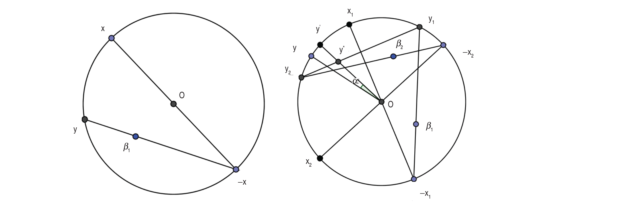
The regression function, which is a form of Möbius transformation, is a mapping of unit circle $| z | = 1$ onto itself. Here, β₀ is a rotation parameter while β₁ is a fixed point in the complex plane. The predicted point y given x is the intersection of the unit circle with the line joining −x and β₁. This is shown in Figure 1. The case of $| β_{1} | > 1$ is also discussed by Kato et al. (2008). In this case, first the fixed point is taken to be $\frac{1}{\bar{β_{1}}}$ . Then this point is joined to $\frac{β_{1}}{| β_{1} |} \frac{β_{1}}{| β_{1} |} \bar{x}$ . The intersection of this line with the unit circle is the predicted point y.

In this model, it can be seen that if $| β_{1} |$ is closer to 1, the function results in the y-values concentrating around $\frac{β_{1}}{| β_{1} |}$ . When $| β_{1} | = 0$ , we have $y = β_{0} x$ ; which is just a rotation. Thus, the regression function defined above can be used for regression when there is only rotation and also in the case when there is reflection about any axis.

Figure 1:

Left: Regression model demonstrated for one regressor taking β₀=1; Right: Regression model demonstrated for two regressors

2.2 Identifiability issue in circular–circular regression

Identifiability of a model means that no two sets of parameters give the same distribution. This is important because otherwise there will be various choices of the parameter set which describe the same thing.

Kato et al. (2008) did not consider the identifiability issue of this model. However, the regression curve given by the Möbius transformation is identifiable. This is because for all $| β_{1} | < 1$ , there exists only a single point β₁ inside the disc $| z | < 1$ through which the projection line (the line joining −x and β₁) is taken. The case for $| β_{1} | > 1$ , as discussed in Kato et al. (2008), seems different from the case of $| β_{1} | < 1$ . However, the geometry in this case can also be explained similarly. This can be shown by comparing the individual coordinates of the predicted point from both the geometries. Without loss of generality, we can take β₁ to be lying on the real axis. This is because any orientation of the circle is equivalent to any other orientation by a rotation. After changing the complex plane $π$ to $ℝ^{2}$ , this is directly implied. The intersection of the line joining $- x = (- x_{1}, - x_{2})$ and $β_{1} = (b, 0)$ , where $b \in ℝ$ , with the unit circle is $y = (\frac{x_{1} (1 + b^{2}) + 2 b}{1 + b^{2} + {bx}_{1}}, \frac{x_{2} (1 - b^{2})}{1 + b^{2} + {bx}_{1}})$ . Changing this in the complex form yields $y = \frac{x + β_{1}}{1 + \bar{β_{1}} x}$ . Thus, both the geometries are similar. In both the cases, as the final projection point is unique, the model remains identifiable.

Mathematically, for a given point x and given β₁, taking β₀=1, the predicted point y is the point at the circle which lies on the line joining −x to β₁. Thus, other possible values of $β_{1}^{'} \in π$ which give the same y for this given x can only be the points lying on this line. This is true for all $x \in Ω$ . Hence, for all $x \in Ω$ , the points x, β₁ and $β_{1}^{'}$ should be collinear. But, if we take $x^{'}$ ( $\neq \frac{x + β_{1}}{1 + \bar{β_{1}} x}$ ) $\in Ω$ , then the three points ( $x^{'}, β_{1}, β_{1}^{'}$ ) will again be collinear if and only if $β_{1} = β_{1}^{'}$ . Thus, β₁ is unique and hence the model is identifiable. Here, β₀ is just a rotation parameter which can be dealt with by rotation directly as done in Theorem 7.2 (see the Appendix).

3 Multiple circular regression models

3.1 Model I (MCR1)

Let $θ_{y}, θ_{x_{j}}$ , $j = 1, \dots, k$ , be circular random variables. Our aim is to regress θ_y on $θ_{x_{j}}$ 's. Let $y = exp (i θ_{y})$ and $x_{j} = exp (i θ_{x_{j}})$ for all j. Then, y can be modelled as

y = β_{0} exp [i arg (Σ_{j = 1}^{k} p_{j} \frac{x_{j} + β_{j}}{1 + \bar{β_{j}} x_{j}})] ε,

(3.1)

where

\begin{matrix} arg (\cdot) \in [0, 2 π); β_{0}, ε \in π; | β_{0} |, | ε | = 1; β_{j} \in π; and Σ_{j = 1}^{k} p_{j} = 1; 0 < p_{j} < 1 for \\ j = 1, \dots, k . \end{matrix}

(3.2)

The model is not defined for $x = (x_{1}, x_{2}, \dots, x_{k})$ when $Σ_{j = 1}^{k} p_{j} \frac{x_{j} + β_{j}}{1 + \bar{β_{j}} x_{j}} = 0$ . If $k = 2$ , then, this problem can be overcome if we define $p_{1} \neq 0.5$ . If $k > 2$ , then while checking the maximum of log-likelihood during data analysis, for a particular parameter set, such sample points should be ignored and the maximum likelihood should be divided by the number of sample points considered for any parameter set. The proposed model also becomes unidentifiable when $| β_{j} | = 1$ for all j. This can be rectified by modifying the parameter space such that at least one $| β_{j} | \neq 1$ .

Note that Equation (3.1) is a multiple circular extension of circular–circular regression proposed by Kato et al. (2008).

The case of two regressors is shown in the right panel of Figure 1. Here O is the centre, and

y^{'} = exp [i arg ({py}_{1} + (1 - p) y_{2})], y = β_{0} y^{'},

where

β_{0} = exp (i α)

The examples of such model can be the direction of bird migration regressed on wind direction and time of year when all the three variables are circular in nature.

The proof of identifiability for this model is given in Appendix A.

3.2 Geometry of multiple circular regression

Theorem 7.1 can also be used to improve the fit of the circular–circular regression when there is only one circular covariate. The geometry is shown in the left panel of Figure 1, which is as follows:

Step 1: $x \Rightarrow - x$ .

Step 2: $- x \Rightarrow y^{'}$ passing through β₁.

Step 3: Rotate $y^{'}$ by $θ_{0} = arg (β_{0})$ to obtain y. (In the figure, $β_{0} = 1$ , and hence $y^{'} = y$ .)

In the case of bivariate circular regression as explained in this article, the right panel of Figure 1 shows the regression. The geometry can be described as follows:

Step 1: $x \Rightarrow - x$ .

Step 2: $- x \Rightarrow y_{1}$ passing through β₁.

Step 3: $- x \Rightarrow y_{2}$ passing through β₂.

Step 4: Join y₁ and y₂ and take $y^{'} = {py}_{1} + (1 - p) y_{2}$ .

Step 5: The regressed point $y^{'}$ is the projection of line joining centre O and $y^{'}$ on the circle.

Step 6: Rotate $y^{'}$ by $α = arg (β_{0})$ to get y.

For the general case, we can obtain $y_{1}, y_{2}, \dots, y_{k}$ as given in Steps 3 and 4. Then we can take $y^{'} = Σ_{j = 1}^{k} p_{j} y_{j}$ . Now, the regressed point will be the projection of line joining centre O and $y^{'}$ on the circle, which is $y^{'}$ . Then, as in Step 6, y can be obtained by rotation of $y^{'}$ by $α$ anticlockwise.

Note: The bivariate case and the general case are explained only for $| β_{j} | \leq 1$ . The case of $| β_{j} | > 1$ for any j can be dealt similarly only by incorporating the geometry as described in that case earlier for one regressor for getting the projection point corresponding to that regressor.

3.2.1 Multiple circular regression

The model described above is helpful in the case of multiple circular regressors. After specifying the direction of 0 angle for each covariate, the parameters p_js can be used to gauge the magnitude of effect of each covariate on the response. The higher the value of a particular p_j, the higher is the effect of that particular regressor x_j on the response y. This can be said because p_js are nothing but weight parameters. Thus, the model can also be used to check the relative effect of the regressors on the response variable.

In MCR also, new parameters corresponding to the covariates can be added as specified in single regressor case to get a better fit than before. The removal of the dependency of the parameter p_j's on the orientation of the covariates can be done by adding another parameter A_j for each covariate and hence, the new model can be written as the following:

y = β_{0} exp [i arg (Σ_{j = 1}^{k} p_{j} \frac{A_{j} x_{j} + β_{j}}{1 + \bar{β_{j}} A_{j} x_{j}})] ε,

(3.3)

The regression function can also be written in the form of tangent link function. In such case, the regression function can be written as

θ_{y} = θ_{0} + arg (exp [i arg (Σ_{j = 1}^{k} p_{j} \frac{A_{j} x_{j} + β_{j}}{1 + \bar{β_{j}} A_{j} x_{j}})]) + θ_{ε},

(3.4)

where

A_{j} \in Ω, A_{1} = 1; arg (\cdot) \in [0, 2 π); β_{0}, ε \in π; | β_{0} |, | ε | = 1; β_{j} \in π;

p = (p_{1}, \dots p_{k}) \in R^{k} : Σ_{j = 1}^{k} p_{j} = 1; 0 < p_{j} < 1 for j = 1, \dots, k .

The proof of identifiability of this model proceeds similarly as is done in Theorem 7.1 and Theorem 7.2.

3.2.2 Invariance and rotational equivariance of parameters

Circular regression models must be origin independent. Hence, for every rotation of the covariates and responses, a desirable feature is to get the same predicted mean direction by changing the model parameters. Also, p must be invariant of the rotations. We shall denote the parameters of the previous model by (β₀, A_j's, β_j's, p) and the new model parameters by (β₀(n), A_j(n)'s, β_j(n)'s, p(n)).

The predicted mean direction of an MCR1 model can also be written as

y = \frac{Σ_{j = 1}^{k} p_{j} β_{0} \frac{A_{j} x_{j} + β_{j}}{1 + \bar{β_{j}} A_{j} x_{j}}}{|Σ_{j = 1}^{k} p_{j} β_{0} \frac{A_{j} x_{j} + β_{j}}{1 + \bar{β_{j}} A_{j} x_{j}}|},

(3.5)

where A₁=1. A change in the 0 angle is the same as multiplying by a unit complex number W. It can be seen directly from Equation (3.5) that if the response y is rotated and the new response is Wy, where

| W | = 1

, there exists a model which gives the same prediction if all the parameters are the same except forβ₀. Thus, (Wβ₀, A_j's, β_j's, p) gives the same prediction in the new model as was given by (β₀, A_j's, β_j's, p) in the previous model.

When x₁ is rotated to Wx₁, then the new model parameters which give the same predicted mean direction are $(\bar{W} β_{0}, {WA}_{j}' s, W β_{j}' s, p)$ .

When $x_{j}$ , $j \neq 1$ , is rotated by W, then the new equivalent model parameters are $(β_{0}, A_{1}, \bar{W} A_{2}, \dots, W^{¯} A_{k}, β_{j}' s, p)$ . The meaning of p is completely preserved as it is invariant with respect to any rotation.

Fixing $A_{1} = 1$ means fixing this value with respect to one of the covariates. The model does not depend on which covariate is chosen as $x_{1}$ because if in another case $x_{r}$ $(r \neq 1)$ is chosen as the covariate such that $A_{r} = 1$ is fixed, then the parameters with respect to the new model which give the same predicted mean direction are ( $β_{0} A_{r}, \bar{A_{r}} A_{j}' s, \bar{A_{r}} β_{j}' s, p$ ).

3.3 Multiple circular regression II (MCR2)

The problem with the model MCR1 is that adding a new covariate results in adding four new parameters to the model: $p_{j}, A_{j}, b_{1, j}, b_{2, j}$ , where $β_{j} = (b_{1, j}, b_{2, j})^{T}$ . Thus, we propose an alternative multiple circular–circular regression model having an increase in two parameters per covariate. We write

y = β_{0} \frac{x^{*} + β_{1}}{1 + \bar{β_{1}} x^{*}} ε,

(3.6)

where

x^{*} = \frac{Σ_{j = 1}^{k} p_{j} A_{j} x_{j}}{| Σ_{j = 1}^{k} p_{j} A_{j} x_{j} |} .

(3.7)

The representation in terms of tangent link function is

θ_{y} = θ_{0} + arg (\frac{x^{*} + β_{1}}{1 + \bar{β_{1}} x^{*}}) + θ_{ε} .

(3.8)

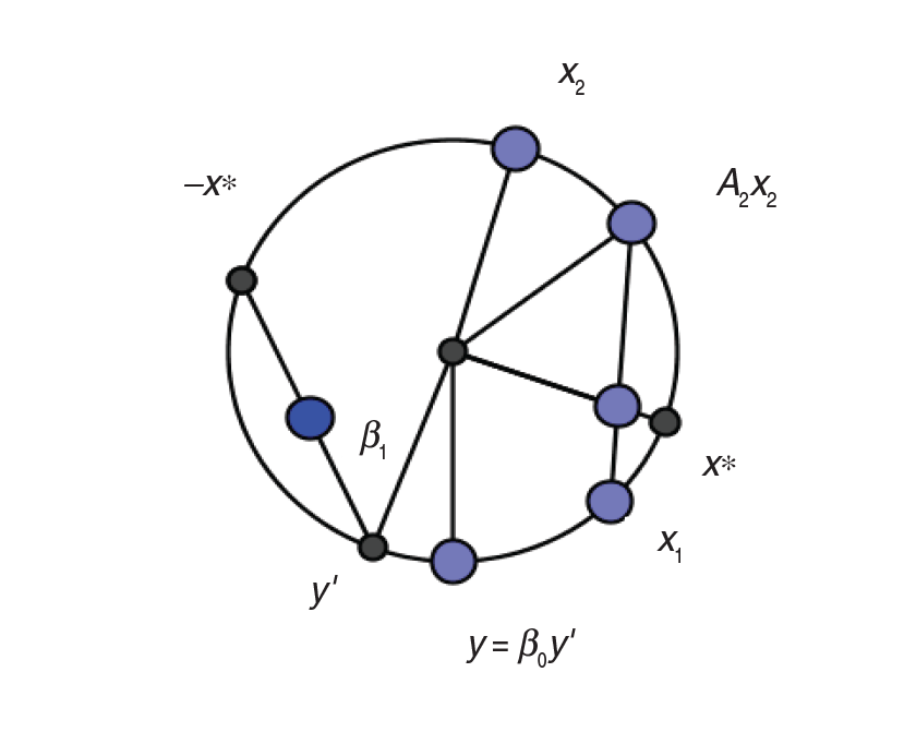
The parameters $p_{j}$ 's, $β_{0}, β_{1}$ , $A_{j}$ 's are defined as earlier. The interpretation of the parameters are the same and the rotational equivariance ofβ₀, $p_{j}$ 's, $A_{j}$ 's is exactly similar to what was discussed in the previous section. By fixing $A_{1} = 1$ , we have locked the location of x₁, hence it can easily be seen that β₁ is rotationally equivariant with x₁. The tangent link function in Downs and Mardia (2002) and the Möbius transformation in Kato et al. (2008) are mathematically equivalent for one covariate. It can be seen that the equivalence of the MCR2 model with Downs and Mardia (2002) is maintained if we consider $x^{*}$ as defined in MCR2 as the covariate in Downs and Mardia (2002). The Figure for the regression function in case of two covariates is shown in Figure 2. The identifiability of this model is proved in Appendix B.

Figure 2:

Regression model demonstrated for two covariates

3.3.1 Invariance and rotational equivariance of parameters

As explained in Section 3.2.2, there must exist an equivalent model with respect to the rotation of the circular variables in MCR2 also. From Equation (3.5), it can be directly seen that if y is rotated by W, then the new model parameters giving the same predicted mean direction as the previous one will be (Wβ₀, A_j's, β₁, p_j's).

Note that Equation (3.6) can also be written as

y = \frac{β_{0} x^{*} + β_{0} β_{1}}{1 + \bar{β_{1}} x^{*}} ε .

Thus, the equivalent new model parameters when x₁ is rotated to Wx₁ are

(W^{¯} β_{0}, A_{1}, {WA}_{j} (j \neq 1), W β_{1}, p_{j}' s)

. When,

x_{j} (j \neq 1)

is rotated to

{Wx}_{j} (j \neq 1)

, then the equivalent new model parameters are

(β_{0}, A_{1}, \dots, \bar{A_{j}}, \dots, A_{k}, β_{1}, p_{j}' s)

The choice of $A_{1} = 1$ does not change the prediction because the equivalent new parameters will then be $(β_{0} A_{r}, \bar{A_{r}} A_{j}, \bar{A_{r}} β_{1}, p_{j}' s)$ .

4 Estimation of parameters

4.1 Maximum likelihood estimators

When $β_{j}$ s are all known for $j = 1, 2, \dots, k$ , and the angular error follows the wrapped Cauchy distribution $WC (ψ)$ , the estimation of $ψ$ andβ₀ can be done by the method proposed by Kent and Tyler (1988). This estimation can also be done by the method of moments as described in Kato et al. (2008). When the angular error follows asymmetric generalized von Mises distribution, then the MCR1 model is of the form

θ_{y} = θ_{0} + θ_{E} + arg (exp [i arg (Σ_{j = 1}^{k} p_{j} \frac{A_{j} x_{j} + β_{j}}{1 + \bar{β_{j}} A_{j} x_{j}})]) + θ_{ε^{'}}

and the MCR2 model can be written as

θ_{y} = θ_{0} + θ_{E} + \arg (\frac{x^{*} + β_{1}}{1 + \bar{β_{1}} x^{*}}) + θ_{ε^{'}} .

In both these cases,

θ_{ε^{'}}

follows AGvM(0,0,1,1) distribution. In this case, when

p_{j}

's,

β_{j}

's and

A_{j}

's are known,

θ_{0} + θ_{E}

can be estimated and then by subtracting the bias in error, the maximum likelihood estimates (MLE) of

θ_{0}

can be obtained, as mentioned in Section 3.3 of Sengupta et al. (2013).

If the angular error follows $VM (0, κ)$ , then the MLEs ofβ₀ and $κ$ reduce to

{\hat{θ}}_{0} = arg (C + iS),

where

arg (\cdot) \in [0, 2 π)

\hat{κ} = A^{- 1} (R / n)

or 0 according as

R / n > 0

or not. If MCR1 is used, then

S = Σ_{r = 1}^{n} sin [θ_{y_{r}} - arg (Σ_{j = 1}^{s} p_{j} \frac{x_{r, j} + β_{j}}{1 + \bar{β_{j}} x_{r, j}})], C = Σ_{r = 1}^{n} cos [θ_{y_{r}} - arg (Σ_{j = 1}^{s} p_{j} \frac{x_{r, j} + β_{j}}{1 + \bar{β_{j}} x_{r, j}})], and R = Σ_{r = 1}^{n} cos [θ_{y_{r}} - {\hat{θ}}_{0} - arg (Σ_{j = 1}^{s} p_{j} \frac{x_{r, j} + β_{j}}{1 + \bar{β_{j}} x_{r, j}})] .

If MCR2 is used, then

S = Σ_{r = 1}^{n} sin [θ_{y_{r}} - arg (\frac{x_{r}^{*} + β_{1}}{1 + \bar{β_{1}} x_{r}^{*}})], C = Σ_{r = 1}^{n} cos [θ_{y_{r}} - arg (\frac{x_{r}^{*} + β_{1}}{1 + \bar{β_{1}} x_{r}^{*}})], and R = Σ_{r = 1}^{n} cos [θ_{y_{r}} - {\hat{θ}}_{0} - arg (\frac{x_{r}^{*} + β_{1}}{1 + \bar{β_{1}} x_{r}^{*}})] .

The maximization of log-likelihood for von Mises case is equivalent to the minimization of circular distances

d_{r} = 1 - cos (θ_{y_{r}} - {\hat{θ}}_{y_{r}})

, between

θ_{y_{r}}

and

{\hat{θ}}_{y_{r}}

, as

L = - n log 2 π - n log (I_{0} (κ)) + κ Σ_{r = 1}^{n} cos (θ_{y_{r}} - {\hat{θ}}_{y_{r}}),

(4.1)

where

θ_{y_{e, j}}

is the estimated value corresponding to the jth regressor. Therefore, for any value of κ, the likelihood is maximized when the circular distance is minimized. Thus, instead of maximizing the more complicated log-likelihood function, the circular distance function can be minimized and then estimate of

κ

can be found through the estimates of

β_{j}

's and

p_{j}

's.

Now, for the first model, $Σ_{r = 1}^{n} cos (θ_{y_{r}} - {\hat{θ}}_{y_{r}})$ is maximized when $θ_{0}$ is the circular mean of $[θ_{y_{r}} - arg (Σ_{j = 1}^{s} p_{j} \frac{x_{r, j} + β_{r, j}}{1 + \bar{β_{j}} x_{r, j}})]$ s, and hence this is equivalent to maximizing

Q = |Σ_{r = 1}^{n} \frac{y_{r}}{y_{c, r}}|

where

y_{c, r} = \frac{Σ_{j = 1}^{s} p_{j} \frac{x_{r, j} + β_{r, j}}{1 + \bar{β_{j}} x_{r, j}}}{|Σ_{j = 1}^{s} p_{j} \frac{x_{r, j} + β_{r, j}}{1 + \bar{β_{j}} x_{r, j}}|} .

In case of the second model, $Σ_{r = 1}^{n} cos (θ_{y_{r}} - {\hat{θ}}_{y_{r}})$ is maximized when $θ_{0}$ is the circular mean of $[θ_{y_{r}} - arg (\frac{x_{r}^{*} + β_{1}}{1 + \bar{β_{1}} x})]$ s, and hence this is equivalent to maximizing

Q = |Σ_{r = 1}^{n} \frac{y_{r}}{y_{c, r}}|

where

y_{c, r} = \frac{x_{r}^{*} + β_{1}}{1 + \bar{β_{1}} x_{r}^{*}} .

Finding the maximum likelihood numerically is not easy in these models because of the presence of many local maxima. The presence of local maxima in case of a specific example can be seen from Figure 3. In the Figure, we have taken the case of the MCR2 model and shown the behaviour of likelihood function with the change of parameters by fixing all but one parameter and changing the non-fixed parameter. The parameters considered are

β_{0} = A_{1} = 1

β_{1} = (0.3, 0)

and

p = 0.3

. From the figure, it can be seen that the likelihood has local maxima both for b₁ and b₂. Both the local maxima can be seen as small spikes on the left of the global maximum. The figure at the right hand side in the second row shows the local maximum at b₂ where the likelihood function is plotted near the local maxima. A similar figure can be obtained on plotting the likelihood near the local maximum for the graph b₁ versus L. Thus, gradient-descent method for finding the global maximum of the likelihood function may not converge to appropriate point. Thus, while using the gradient-descent methods, different initial values should be taken for the parameters.

Figure 3:

Plots for Likelihood Function. [Top row:] Graphs of likelihood (L) against (Left:) $A_{θ_{0}}$ and (Right:) b₁. [Middle row:] Graphs of likelihood (L) against (Left:) b₂ and (Right:) b₂ near the local maximum. [Bottom row:] Graph of likelihood (L) against $p$

Another very useful alternative for finding the global maximum is to use the bootstrap restarting method discussed in Wood (2001). The steps required for approximating the MLE by bootstrap restarting for our set-up are the following:

Step 1: Take an initial parameter set q₀.

Step 2: Starting from q₀, find a local maximum q_i and calculate $L (q_{i}, x, y)$ , the log-likelihood function.

Step 3: Take a bootstrap sample $(y^{*}, x^{*})$ from the dataset.

Step 4: Find $q_{i}^{*}$ taking $q_{i}$ as the starting parameter.

Step 5: Check if $L (q_{i}^{*}, x, y) > L (q_{i}, x, y)$ . If it is so, then take $q_{0} = q_{i} * = q_{i + 1}$ , else take $q_{0} = q_{i}$ and repeat the steps from 1 to 5 until convergence.

As already mentioned, for the parameter set, taking the parameters related to are enough because we can get the MLE of β0 and $κ$ directly from these parameters.

4.2 Fisher information matrix

If angular error follows $VM (0, κ)$ , then $- E (\frac{d^{2} L}{d κ^{2}}) = n \frac{d}{d κ} A (κ)$ , $- E (\frac{d^{2} L}{d θ_{0}^{2}}) = {nkI}_{1} (κ)$ , and

- E (\frac{d^{2} L}{d θ_{0} d κ}) = - E (\frac{d^{2} L}{d θ_{j} d κ}) = - E (\frac{d^{2} L}{{dr}_{j} d κ}) = - E (\frac{d^{2} L}{{dp}_{j} d κ}) = 0 .

Hence, asymptotically, the MLE of

κ

and the MLEs of

θ_{0}, θ_{j}, p_{j}, r_{j}

for all j will be independent. Other terms of the Fisher information matrix can be found numerically as the equations are very complex.

Similarly, if the angular error follows $C^{*} (ψ)$ , then

- E (\frac{d^{2} L}{d ψ d θ_{0}}) = - E (\frac{d^{2} L}{d ψ d θ_{k}}) = - E (\frac{d^{2} L}{d ψ {dr}_{k}}) = - E (\frac{d^{2} L}{d ψ {dp}_{k}}) = 0 .

Thus, the MLE of ψ will be asymptotically independent of the MLEs of

θ_{0}, θ_{k}, r_{k}, p_{k}

for all k. Other terms of the matrix can be similarly obtained, although some of the functions are very complex and they can be computed numerically.

4.3 Improving the fit in case of single regressor

In case of circular–circular regression of Kato et al. (2008), one circular variable is regressed on only one circular regressor. The fit of the regression can be improved by using the model proposed in the article by adding one new parameter $β_{j}$ and correspondingly $p_{j}$ at each step and calculating the accuracy in terms of the sum of cosines of the angles between the fitted and observed value. A new pair of parameters $(β_{j}, p_{j})$ can be added till the improvement in fitting is more than a predefined value. This is similar to adding the powers of x in the linear regression case so that the fitting is improved. This case can also be equated to the case when in multiple linear regression, orthogonal polynomials of the regressor x are added and penalty is calculated until the improvement in fitting is less than a predefined value. Here, also a method similar to adjusted $R^{2}$ may be used to calculate the optimum number of $β_{j}$ s.

Here we intend to define the circular version of $R^{2}$ statistic, and denote it by $R_{C}^{2}$ . For illustration, we assume that $arg (ε_{j})$ follows $VM (0, κ)$ distribution, the von Mises distribution with location 0 and concentration parameter $κ$ , with probability density function (pdf) given by

f_{0, κ} (z) = \frac{1}{2 π I_{0} (κ)} exp (κ cos (z)),

where

0 \leq z < 2 π

, and

κ > 0

, and

I_{j} (κ) = \frac{1}{π} \int_{0}^{π} exp (κ cos z) cos (j z) dz,

the modified Bessel function of the first kind of order

j \geq 0

. Denote

A (κ) = I_{1} (κ) / I_{0} (κ)

. As

κ

is the concentration parameter, higher value of

κ

indicates a better fit. Here

\hat{κ}

, the MLE of

κ

, comes out to be

\hat{κ} = \{\begin{matrix} A^{- 1} (\frac{1}{n} Σ_{r = 1}^{n} cos {\hat{θ}}_{ε_{r}}), & if Σ_{i = 1}^{n} cos {\hat{θ}}_{ε_{r}} > 0, \\ 0 & otherwise, \end{matrix}

where

ε_{r} = exp (i θ_{ε_{r}})

and

{\hat{θ}}_{ε_{r}}

is the estimated value of

θ_{ε_{r}}

from the data. Now, note that

A (κ)

is a monotonically increasing function of

κ

. Thus,

R_{C}^{2}

can be used to check the goodness of fit of the model, which is similar to

R^{2}

in the linear case, where

R_{C}^{2} = \frac{1}{2} (1 + \frac{1}{n} Σ_{r = 1}^{n} cos {\hat{θ}}_{ε_{r}}) .

Here

{\hat{θ}}_{ε_{r}} = arg ({\hat{ε}}_{r}) \in [0, 2 π)

. It can be easily seen that the value of

R_{C}^{2}

lies in

[0, 1]

, and

R_{C}^{2}

is larger for a better fit. In fact,

R_{C}^{2} = 1

for a perfect fit (where

{\hat{θ}}_{ε_{r}} = 0

for all

r

), and

R_{C}^{2} = 0

for a disastrous fit (where

{\hat{θ}}_{ε_{r}} = π

, the maximum possible departure, for all

r

). There is one big difference between

R_{C}^{2}

and

R^{2}

because unlike in the linear case,

R_{C}^{2}

does not incorporate the percentage of variation due to the difference in decomposition of cosine and squared functions.

However, a more objective method to check the significance of change can be through the log-likelihood. Given the model and assuming angular error following $VM (0, κ)$ distribution, the likelihood based testing for the addition of parameters can be done in the following way. Under the model given in equations (3.1) and (3.2), the log-likelihood ratio test statistic for $H_{0} : p_{s} = 0$ against $H_{1} : p_{s} \neq 0$ can be used to check for any significant difference by adding new parameter $β_{s}$ .

Let $ℓ_{0}$ denote the maximum of log-likelihood of y given x under $H_{0}$ , and $ℓ_{1}$ denote the same under $H_{1}$ . For using Likelihood Ratio Test (LRT), we need to find the distribution of $Λ = - 2 (ℓ_{0} - ℓ_{1})$ . However, if $p_{s} = 0$ , then the parameter $β_{s}$ becomes unidentifiable. This is because $β_{s}$ can take any value when $p_{s} = 0$ . Moreover, even if $p_{s} \neq 0$ and $β_{s}$ is equal to any one of $β_{1}, \dots, β_{s - 1}$ , then the parameters $p_{j}$ 's become non-identifiable. Hence, the regularity condition of model identifiability for the standard asymptotic chi-squared distribution of the LRT statistic is not satisfied by the model under null hypothesis. Thus, we need an alternative approach.

McLachlan (1987) discussed a problem where the LRT statistic was bootstrapped to estimate the number of components in a normal mixture. Here, we consider a similar methodology in our article. First, based on the sample, MLEs of the model parameters were found using $(s - 1)$ number of $β$ 's, and for the same sample, MLEs were found by using $s$ number of $β$ 's. Based on the estimates from the first model, $K$ bootstrap samples of the same sample size as of the original sample were generated. Our case is a bit different from McLachlan (1987) as the bootstrap sample is bivariate $(θ_{x}, θ_{y})$ . Let the distribution of $θ_{x}$ be known. Then, an independent bootstrap sample for $θ_{x}$ is generated from the distribution of $θ_{x}$ . This generation of $θ_{x}$ from its distribution is considered because then the fitted model will not only be good for the sample data but it will be good over the whole sample space of $θ_{x}$ . Based on each of these $θ_{x}$ , $θ_{y}$ is generated using the estimates $\hat{Φ}$ based on the model under null hypothesis. This bootstrap sample hence obtained is used to estimate the parameters under both the models. The same process is repeated independently $K$ times, and $Λ$ is calculated each time. The value of the jth order statistic of the $K$ replications can be taken as an estimator of the quantile of order $j / (K + 1)$ , and the $P$ -value can be assessed with respect to the ordered bootstrap replications of $Λ$ .

Under the assumption of von Mises distribution for angular error,

- 2 (ℓ_{0} - ℓ_{1}) = 2 n [log (I_{0} ({\hat{κ}}_{s - 1}) - {\hat{κ}}_{s - 1} A ({\hat{κ}}_{s - 1}) - log (I_{0} ({\hat{κ}}_{s}) + {\hat{κ}}_{s} A ({\hat{κ}}_{s})] .

Now,

\hat{κ}

is an increasing function of

R_{C}^{2}

. As

A (κ)

is a strictly increasing function of

κ

for

κ > 0

, we have

\frac{dA (κ)}{d κ} > 0

. Hence,

\frac{d}{d κ} [log (I_{0} (κ)) - κ A (κ)] = - κ \frac{dA (κ)}{d κ}

indicates that

log (I_{0} (κ)) - κ A (κ)

is a decreasing function of

κ

. Thus, the higher the difference between successive

R_{C}^{2}

's, the higher the significance of new parameter. The value of

Λ

also explains if there is any significant reduction in

R_{C}^{2}

when new parameter is added.

Other circular distributions for $ε$ will work as well. One such example can be the wrapped Cauchy distribution as described earlier by Kato et al. (2008). When angular error follows the wrapped Cauchy distribution with 0 mean, then arg( $ε) \sim C^{*} (ψ)$ , where $0 \leq ψ \leq 1$ . In this case, the model is a good fit if $ψ$ is closer to 1.

Standard model selection criteria like the bias-corrected Akaike information criterion (AICC) can also be used to select the appropriate candidate for the model; see Lund (1999) in this context. For von Mises error distribution,

AICC = 2 n log I_{0} (\hat{κ}) - 2 n \hat{κ} + \frac{n (n + l)}{n - l - 2},

where

l

is the number of parameters estimated for the mean direction.

4.4 Donut-plot

A new type of plot is also introduced in this present article. This plot is called donut-plot. The problem with normal x versus y graph in circular cases is that it depends on the choice of ‘0’. The spokeplot, introduced by Zubairi et al. (2008) and as shown in Kato et al. (2008), is a very good pictorial representation of observed versus estimated values. But, when the sample size is large, usually a lot of lines criss-cross each other and in that case the plot is not very clear. See the spokeplot at the left in the bottom row of Figure 5.

The donut-plot is used to plot the estimated value and the corresponding observed value. Let the estimated angle be $θ_{y_{e}}$ and the observed angle be $θ_{y}$ . Then, this plot shows the point $(1 + cos (θ_{y_{e}} - θ_{y})) (cos θ_{y_{e}}, sin θ_{y_{e}})$ . Thus, if the fit is good, then more points will be near the circumference of the circle with centre at 0 and radius =2, while a bad fit results in more points inside the unit radius disc. Here, as in spokeplot, we do not need to delete the outliers. The donut-plot can be further improved by using different coloured dots for clockwise and anticlockwise deviations. This is because it also shows the direction in which the estimated points are deviating from the observed values. In the donut-plots given in Section 5, we have used solid circles for clockwise deviations and empty circles for anticlockwise deviations. Thus, the donut-plot provides an alternative to the x versus y graph and the spokeplot.

4.5 Simulation

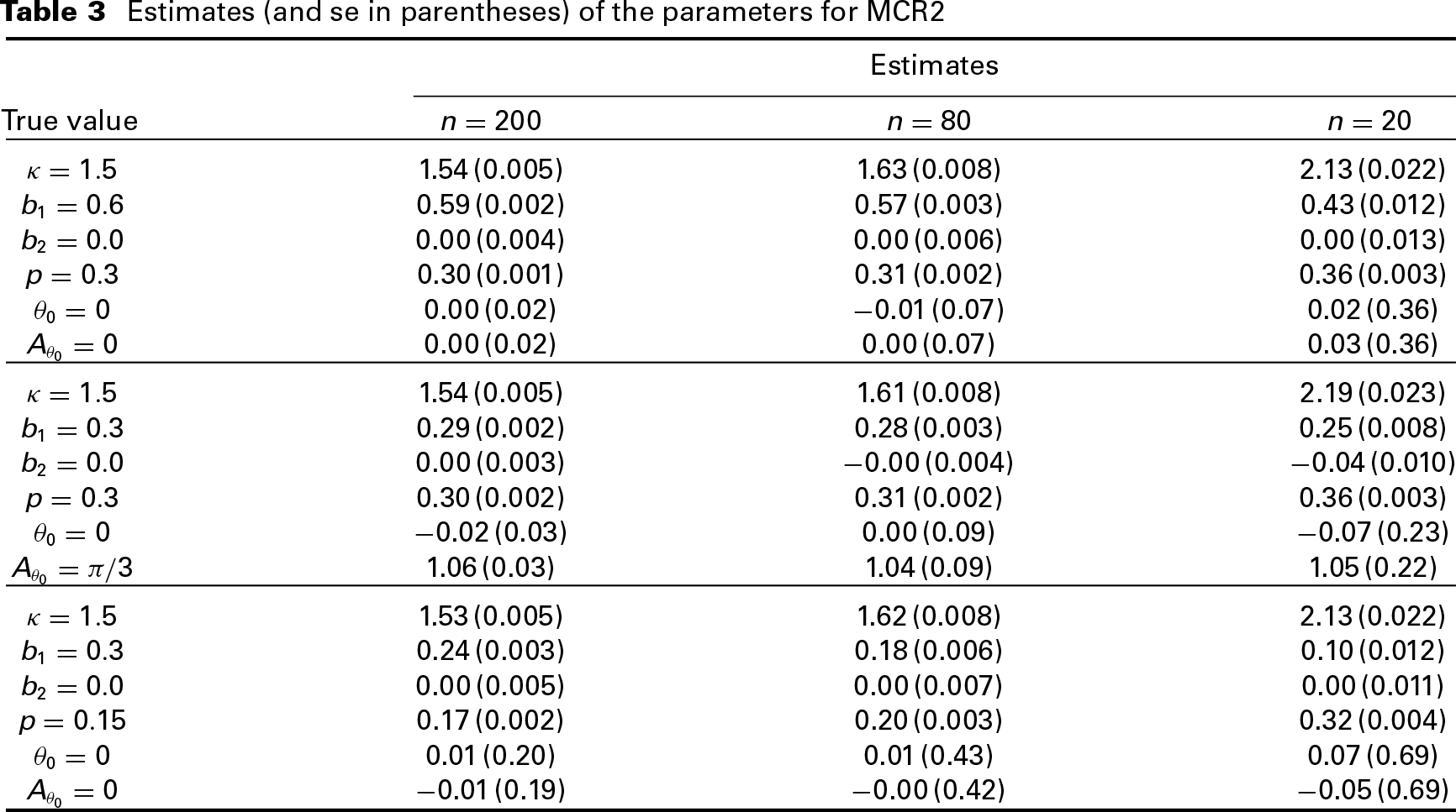
Simulation studies are done for the MCR case when the angular variable $θ_{y}$ is regressed on two independent angular covariates $θ_{x_{1}}$ and $θ_{x_{2}}$ . The simulation is performed both for the MCR1 and MCR2 models. The method employed for finding the global maximum in this article is by giving different initial values to the optim function in R. The simulation results, for the MCR1 model, are shown in Table 1 and the simulation results for the MCR2 model are shown in Tables 2 and 3. Table 1 shows the estimates when the data is generated from the MCR1 model and estimates are the MLE based on the MCR1 model. Table 2 shows the estimates when the data is generated from the MCR2 model and estimates are the MLE based on the MCR2 model. In the tables, the sample standard errors (se's) for the estimates of linear variables and sample circular variances for the estimates of circular variables are given in parentheses. The definition of sample circular variance is the one used in equation (2.3.3) of Mardia and Jupp (2000). The sample circular variance is $1 - \bar{R}$ , where $\bar{R}$ is the mean resultant length of the unit complex numbers corresponding to the MLEs of the circular parameters. The mean of the estimates are the mean of MLE found from 1 000 runs and the standard deviations (SDs) are the SD of the MLEs found from the 1 000 runs. Consequently the se's are calculated. We carried out extensive computations, but reported the results for only three parameter combinations and for sample sizes 20 (small sample case, similar to Example 1 in Section 5.1), 80 (moderate sample size, close to the situation of Example 2 of Section 5.2), and 200 (large sample case). The estimates are quite close, even for a small sample case, and the estimates improve as the sample size increases. However, the estimate of $κ$ is not quite good when the sample size is small (like 20), the estimate improves with the increase in sample size. For the MCR2 model, we have also changed p and it can be seen from Table 2 and Table 3 that for low p, the se's of the MLEs are high.

In Table 1, β₁ and $β_{2}$ are represented by $(b_{11}, b_{12})$ and $(b_{21}, b_{22})$ , respectively, $A_{θ_{0}}$ represent the argument of $A_{2}$ , $θ_{0}$ gives the argument ofβ₀ and p represents the weight of the first covariate. In Table 2, $(b_{1}, b_{2})$ represents β₁, $θ_{0}$ is the argument ofβ₀, p is the weight $p_{1}$ of the first covariate and $A_{θ_{0}}$ is the argument of $A_{2}$ .

Table 1:

Estimates (and se in parentheses) of the parameters for MCR1

	Estimates
True value	n=200	n=80	n=20
κ=3	3.095 (0.009)	3.318 (0.015)	5.621 (0.080)
b₁₁=0.7	0.707 (0.002)	0.704 (0.005)	0.572 (0.012)
b₁₂=0	0.000 (0.002)	0.002 (0.005)	−0.003 (0.012)
b₂₁=0.5	0.459 (0.005)	0.389 (0.005)	0.225 (0.011)
b₂₂=0	0.005 (0.006)	0.003 (0.009)	0.001 (0.013)
p=0.4	0.411 (0.001)	0.427 (0.001)	0.449 (0.002)
A_θ0=0	0.008 (0.036)	0.003 (0.104)	0.009 (0.302)
θ₀=0	−0.005 (0.018)	0.001 (0.049)	−0.002 (0.182)
κ=3	3.101 (0.008)	3.337 (0.015)	5.634 (0.090)
b₁₁=0.7	0.707 (0.002)	0.710 (0.005)	0.585 (0.012)
b₁₂=0	0.006 (0.002)	0.004 (0.005)	0.003 (0.012)
b₂₁=0.5	0.461 (0.002)	0.386 (0.005)	0.217 (0.011)
b₂₂=0	−0.015 (0.005)	0.015 (0.009)	0.016 (0.014)
p=0.4	0.411 (0.001)	0.430 (0.001)	0.449 (0.002)
A_θ0=π/3	1.024 (0.034)	1.067 (0.109)	1.085 (0.336)
θ₀=0	0.015 (0.017)	−0.020 (0.053)	−0.025 (0.206)
κ=1.5	1.564 (0.005)	1.729 (0.008)	2.837 (0.038)
b₁₁=0.7	0.706 (0.005)	0.670 (0.008)	0.517 (0.015)
b₁₂=0	0.002 (0.005)	−0.006 (0.008)	0.013 (0.014)
b₂₁=0.5	0.388 (0.005)	0.282 (0.008)	0.187 (0.014)
b₂₂=0	0.001 (0.009)	0.010 (0.012)	−0.009 (0.015)
p=0.4	0.432 (0.001)	0.451 (0.001)	0.470 (0.001)
A_θ0=0	0.004 (0.102)	0.032 (0.222)	0.010 (0.338)
θ₀=0	−0.008 (0.050)	−0.022 (0.116)	−0.006 (0.239)

Table 2:

Estimates (and se in parentheses) of the parameters for MCR2

	Estimates
True value	n=200	n=80	n=20
κ=3	3.08 (0.009)	3.21 (0.015)	4.32 (0.051)
b₁=0.3	0.28 (0.001)	0.25 (0.003)	0.14 (0.007)
b₂=0.0	0.00 (0.003)	−0.01 (0.005)	−0.01 (0.008)
p=0.15	0.16 (0.001)	0.14 (0.002)	0.24 (0.003)
θ₀=0	−0.01 (0.07)	0.03 (0.2)	0.02 (0.55)
A_θ0=0	0.01 (0.07)	−0.02 (0.2)	−0.03 (0.55)
κ=3	3.06 (0.008)	3.22 (0.015)	4.32 (0.053)
b₁=0.6	0.60 (0.001)	0.59 (0.002)	0.52 (0.004)
b₂=0.0	0.00 (0.002)	0.00 (0.003)	−0.03 (0.006)
p=0.25	0.25 (0.001)	0.25 (0.002)	0.28 (0.003)
θ₀=0	0.00 (0.01)	−0.00 (0.04)	−0.04 (0.15)
A_θ0=0	0.00 (0.01)	−0.00 (0.04)	0.02 (0.19)
κ=3	3.08 (0.008)	3.22 (0.015)	4.23 (0.051)
b₁=0.3	0.30 (0.001)	0.30 (0.002)	0.28 (0.009)
b₂=0.0	0.00 (0.002)	0.00 (0.003)	0.02 (0.005)
p=0.3	0.30 (0.001)	0.30 (0.001)	0.32 (0.003)
θ₀=0	0.01 (0.01)	−0.02 (0.02)	0.02 (0.13)
A_θ0=π/3	1.04 (0.01)	1.06 (0.02)	1.04 (0.13)

Table 3:

Estimates (and se in parentheses) of the parameters for MCR2

	Estimates
True value	n=200	n=80	n=20
κ=1.5	1.54 (0.005)	1.63 (0.008)	2.13 (0.022)
b₁=0.6	0.59 (0.002)	0.57 (0.003)	0.43 (0.012)
b₂=0.0	0.00 (0.004)	0.00 (0.006)	0.00 (0.013)
p=0.3	0.30 (0.001)	0.31 (0.002)	0.36 (0.003)
θ₀=0	0.00 (0.02)	−0.01 (0.07)	0.02 (0.36)
A_θ0=0	0.00 (0.02)	0.00 (0.07)	0.03 (0.36)
κ=1.5	1.54 (0.005)	1.61 (0.008)	2.19 (0.023)
b₁=0.3	0.29 (0.002)	0.28 (0.003)	0.25 (0.008)
b₂=0.0	0.00 (0.003)	−0.00 (0.004)	−0.04 (0.010)
p=0.3	0.30 (0.002)	0.31 (0.002)	0.36 (0.003)
θ₀=0	−0.02 (0.03)	0.00 (0.09)	−0.07 (0.23)
A_θ0=π/3	1.06 (0.03)	1.04 (0.09)	1.05 (0.22)
κ=1.5	1.53 (0.005)	1.62 (0.008)	2.13 (0.022)
b₁=0.3	0.24 (0.003)	0.18 (0.006)	0.10 (0.012)
b₂=0.0	0.00 (0.005)	0.00 (0.007)	0.00 (0.011)
p=0.15	0.17 (0.002)	0.20 (0.003)	0.32 (0.004)
θ₀=0	0.01 (0.20)	0.01 (0.43)	0.07 (0.69)
A_θ0=0	−0.01 (0.19)	−0.00 (0.42)	−0.05 (0.69)

4.5.1 Simulation for robustness

In this article, we have considered von Mises distribution for angular error. Kato et al. (2008) used the wrapped Cauchy distribution for angular error. Cauchy distribution is a heavy-tailed distribution. Thus, we have compared the case when the angular error follows von Mises distribution with zero mean to the case when the angular error follows the wrapped Cauchy distribution with real parameter. We have simulated the data from the MCR2 model for this comparison. We have used an accuracy measure mentioned below for checking which among the wrapped Cauchy and von Mises distribution is more robust distribution for the error. For this, first we have taken the true distribution of angular error to be von Mises and then found the accuracy at different sample sizes by assuming both the wrapped Cauchy and von Mises distribution for the angular error. Then, we have taken the wrapped Cauchy distribution as the true distribution for the angular error and then again found the accuracy assuming both the wrapped Cauchy distribution as well as von Mises distribution for angular error.

Table 4:

Accuracy values when angular error follows von Mises distribution

,	n=20		n=80		n=200
κ	VM	WC	VM	WC	VM	WC
1.5	121.17	119.87	49.77	48.71	14.56	12.62
3	163.15	162.19	66.05	64.97	17.44	16.34
4.5	176.71	176.26	79.97	70.47	18.22	17.65
6	182.71	182.49	73.35	73.06	18.67	18.21

For all the simulations, true parameter values are fixed at $β_{1} = 0.3$ , $p = 0.3$ , $β_{0} = 1$ and $A_{2} = 1$ . In Table 4, the error follows von Mises distribution with zero mean direction and different values of the concentration parameter $(κ = 1.5, 3, 4.5, 6)$ . For each of these cases, 1 000 simulations are done at three sample sizes $(n = 20, 80, 200)$ . The robustness is measured with respect to the total accuracy in prediction. The total accuracy is defined as the sum of cosines of the angles between the predicted mean direction and the observed mean direction, that is,

Accuracy = Σ_{i = 1}^{n} cos (θ_{y_{r}} - {\hat{θ}}_{y_{r}}) .

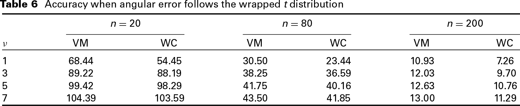
The mean value of the Accuracy over 1 000 simulations is used to check the robustness. This accuracy measure is defined using circular distance, see Sengupta et al. (2013) for details. In Table 5, the distribution for angular error is considered to be the wrapped Cauchy with different values of parameter

(ρ = 0.2, 0.4, 0.6, 0.8)

at the above mentioned sample sizes. For each of the cases, 1 000 simulations are done and the total accuracy is found by assuming that the angular error follows the wrapped Cauchy and then by assuming that the angular error follows the von Mises distribution. Then, we have taken the case when angular error follows the wrapped

t

distribution with the scale parameter 1 and mean as 0 at different degrees of freedom (

ν = 1, 3, 5, 7)

at different sample sizes. Then, we have obtained the mean total accuracy based on 1 000 simulations by assuming first that the angular error follows wrapped Cauchy distribution and again assuming that the angular error follows von Mises distribution. The results are given in Table 6. Note that

ν = 1

for the wrapped

t

reduces to wrapped Cauchy with

ρ = e^{- 1} ≃ 0.368

, and the performance of the wrapped

t

for

ν = 1

in Table 6 is expected to be in between those corresponding to

ρ = 0.2

and

ρ = 0.4

in Table 5, closer to the case corresponding to

ρ = 0.4

. Our results are obtained accordingly.

From the results in Tables 4, 5 and 6, it can be seen that the von Mises distribution not only gives better results than the wrapped Cauchy distribution when the true density of the angular error is von Mises but also when the true density is the wrapped Cauchy or the wrapped $t$ . This might be for our specific choice of Accuracy, which is a term in the expression of the log-likelihood for von Mises distribution we maximize to find the MLE of von Mises parameters; see Equation (4.3).

Table 5:

Accuracy when angular error follows the wrapped Cauchy distribution

,	n=20		n=80		n=200
ρ	VM	WC	VM	WC	VM	WC
0.2	46.91	45.70	23.76	20.96	10.09	7.12
0.4	82.53	81.33	34.98	34.28	11.51	9.65
0.6	121.29	121.23	49.49	48.52	14.02	12.73
0.8	160.41	159.73	64.52	64.24	16.72	16.08

Table 6:

Accuracy when angular error follows the wrapped t distribution

,	n=20		n=80		n=200
ν	VM	WC	VM	WC	VM	WC
1	68.44	54.45	30.50	23.44	10.93	7.26
3	89.22	88.19	38.25	36.59	12.03	9.70
5	99.42	98.29	41.75	40.16	12.63	10.76
7	104.39	103.59	43.50	41.85	13.00	11.29

5 Data analysis

5.1 Example: Single regressor

The data analysis for the case of one circular regressor and one circular response variable is used here to show the advantage of the model in improving the fit in the case of a single regressor. The data were also used in Kato et al. (2008). The wind direction was measured each day at a weather station in Milwaukee for 21 consecutive days at 6 a.m. and 12 noon (Johnson and Wherly (1977), Table 2). The response variable is the wind direction at 12 noon and the covariate is the wind direction at 6 a.m. Watson's test (1983) indicates no significant departure of the angular error from $VM (0, κ)$ distributions in both one parameter and two parameter cases at 1% significance level (p-values are 0.248 and 0.523, respectively).

The MLEs for the parameters when only one $β_{j}$ is used, come out to be: ${\hat{β}}_{1} = 0.055 + 0.259 i$ , ${\hat{β}}_{0} = 0.753 + 0.658 i$ , $\hat{κ} = 1.113$ and $R_{c, 1}^{2} = 0.743$ . Here, the estimate of β₁ is obtained using the estimates of $r$ and $θ_{1}$ .

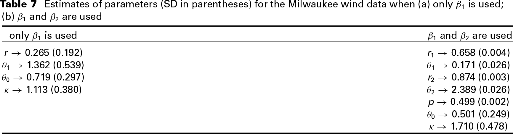
When both β₁ and $β_{2}$ are considered in the model, the MLE for the parameters come out to be ${\hat{β}}_{1} = -$ 0.637 +0.597i, ${\hat{β}}_{2} = 0.648 + 0.113 i$ , ${\hat{β}}_{0} = 0.878 + 0.478 i$ , $\hat{p} = 0.501$ , $\hat{κ} = 1.710$ and $R_{c, 2}^{2} = 0.823$ . Here, β₁ and $β_{2}$ are estimated by taking $β_{1} = r_{1} e^{i θ_{1}}$ and $β_{2} = r_{2} e^{i θ_{2}}$ and then estimating the values of $r_{1}, r_{2}, θ_{1}, θ_{2}$ . The estimates of all the parameters are given in Table 7.

The estimates of SD of the parameters reported in the tables are found by taking the inverse of the hessian matrix at the MLEs.

Table 7:

Estimates of parameters (SD in parentheses) for the Milwaukee wind data when (a) only β₁ is used; (b) β₁ and β₂ are used

only β₁ is used	β₁ and β₂ are used
r→ 0.265 (0.192)	r₁→ 0.658 (0.004)
θ₁→ 1.362 (0.539)	θ₁→ 0.171 (0.026)
θ₀→ 0.719 (0.297)	r₂→ 0.874 (0.003)
κ→ 1.113 (0.380)	θ₂→ 2.389 (0.026)
	p→ 0.499 (0.002)
	θ₀→ 0.501 (0.249)
	κ→ 1.710 (0.478)

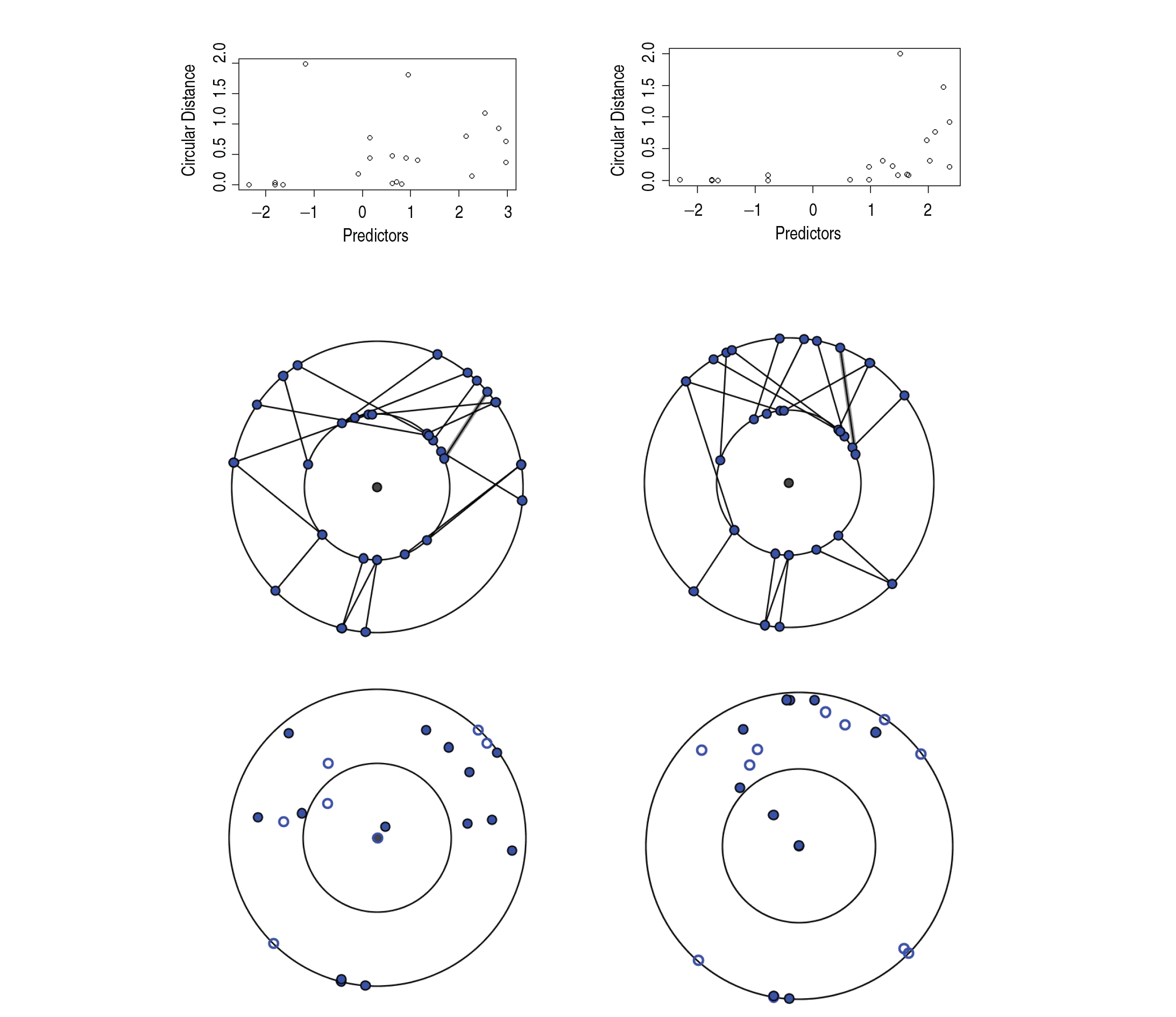
By looking at $R_{c, 1}^{2}$ and $R_{c, 2}^{2}$ , it can be said that the second model fits the data better than the first one. The graph between circular distance ( $1 - cos (θ_{y_{e}} - θ_{y}$ )), and predictors for both the cases are shown in the top row of Figure 4. Comparing the two plots, it can be said that the fit is better in the second case. Then, the bootstrapping procedure for $Λ$ was used to approximate the true distribution of $Λ$ under the null hypothesis as described in Section 4.3 with $K = 25$ . First, Watson's test was performed on the data and it could not reject uniformity for $θ_{x}$ . Then, $θ_{y}$ 's were generated based on $θ_{x}$ 's generated from uniform distribution over $[0, 2 π)$ . The estimate of 0.95-sample quantile based on 25 such bootstrapping comes to be 12.629 and the 0.9-sample quantile estimate comes to be 9.137. The observed value of Λ from the sample is 9.265. Hence, the choice of the first model is not rejected at 5% significance level while the null hypothesis is rejected and the second model is chosen at the 10% significance level. The AICC statistic as defined in Lund (1999) is −3.126 and −1.775 for the first and the second cases, respectively, showing the preference for the first model, but the difference is not large.

The spokeplots are shown in the middle row of Figure 4, while the proposed donut-plots are shown in the bottom row of Figure 4. The left figure in each row corresponds to the model with only one β, and the right hand figure is for two βs. The R codes of this data analysis can be obtained from the authors upon request.

Figure 4:

Plots for Milwaukee data. [Top row:] Graph of circular distance versus predictors when (Left:) only β₁ is used and when (Right:) $β_{1}, β_{2}$ are used. [Middle row:] Spokeplot when (Left:) only β₁ is used and when (Right:) β₁ and $β_{2}$ are used. [Bottom row:] Donut-plot when (Left:) only β₁ is used and when (Right:) β₁ and $β_{2}$ are used

5.2 Example: Multiple regressors

We consider a similar weather data with one circular response and two circular covariates to illustrate the MCR application of the model. The data used is the wind direction data in Ambikapur district of Chhattisgarh from September 2011 to June 2012. The data is taken from the website of Agricultural Meteorology Division, India Meteorological Department, Ministry of Earth Sciences (http://www.imdagrimet.gov.in/winddirection). The dataset consists of 81 points, each corresponding to a different date and a particular hourly time corresponding to the date. The circular covariates considered here are the the date of the year and the time of the day. For the time of the day, 00:00 hrs is considered to be the zero angle; for the time of the year, 8th June (the date corresponding to the first data point) is considered to be the zero angle. Data analysis is done for both the MCR1 and MCR2 models.

Figure 5:

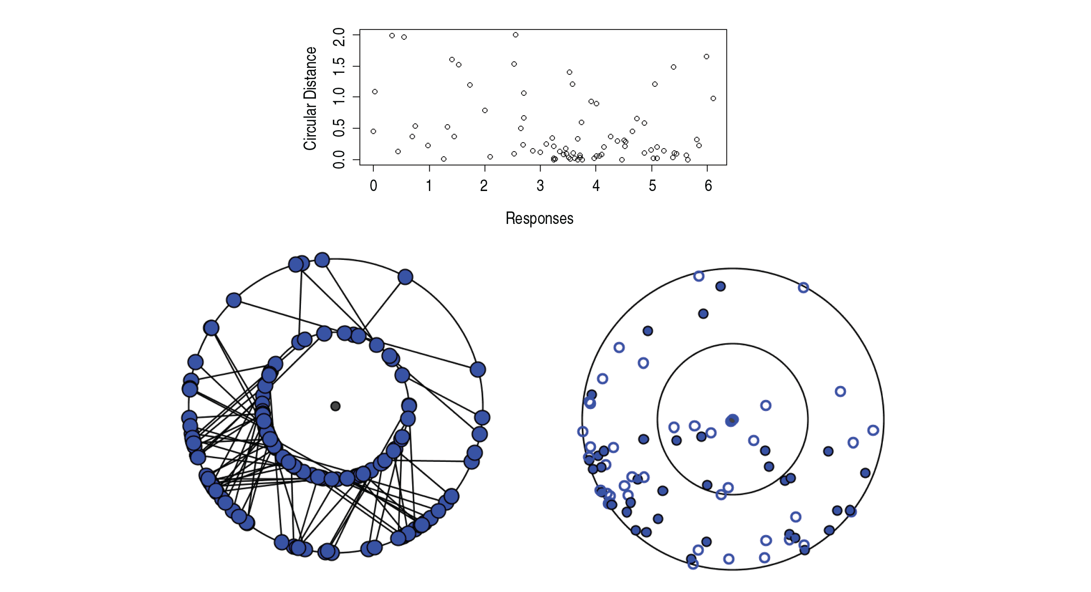
Plots for Chhattisgarh data. [Top row:] Graph of circular distance versus predictors. [Bottom row:] (Left:) Spokeplot; (Right:) Donut-plot

Figure 6:

Plots for Chhattisgarh data.(MCR2) [Top row:] Graph of circular distance versus predictors. [Bottom row:] (Left:) Spokeplot; (Right:) Donut-plot

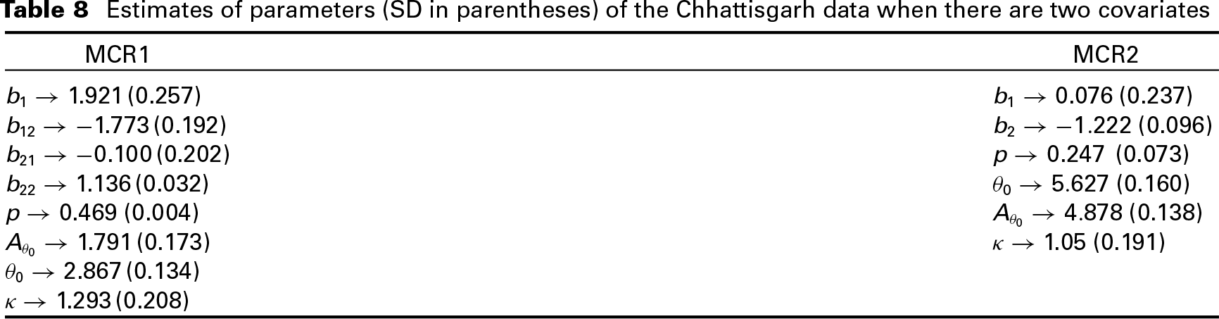
In case of MCR1 model, the goodness of fit test using Watson's test (1983) indicated no significant departure from the von Mises distribution for the angular error at 1% significance level (p-value $= 0.42$ ). Consequently, the MLEs of the parameters ( $β_{0}, β_{1}, β_{2}, p, κ$ ) are obtained. Here, β₁ is the parameter corresponding to time of the day, and $β_{2}$ is the parameter corresponding to the date of the year. The MLEs of the parameters are: ${\hat{β}}_{0} = - 0.963 + 0.271 i$ , ${\hat{β}}_{1} = 1.921 - 1.773 i$ , ${\hat{A}}_{2} = - 0.218 + 0.976 i$ , ${\hat{β}}_{2} = - 0.1 + 1.136 i$ , $\hat{p} = 0.469$ $\hat{κ} = 1.293$ . The graph between circular distances and response values is shown in the top row of Figure 5. The spokeplot excluding the outliers is shown in the left of the bottom row, while the donut-plot is shown in the bottom right of Figure 5. Here, β₁ and $β_{2}$ are estimated by first taking $β_{1} = r_{1} e^{i θ_{1}}$ and $β_{2} = r_{2} e^{i θ_{2}}$ and then estimating the values of $r_{1}, r_{2}, θ_{1}, θ_{2}$ . The estimates of all the parameters are given in the left panel of Table 8.

Table 8:

Estimates of parameters (SD in parentheses) of the Chhattisgarh data when there are two covariates

MCR1	MCR2
b₁→ 1.921 (0.257)	b₁→ 0.076 (0.237)
b₁₂→ −1.773 (0.192)	b₂→ −1.222 (0.096)
b₂₁→ −0.100 (0.202)	p→ 0.247 (0.073)
b₂₂→ 1.136 (0.032)	θ₀→ 5.627 (0.160)
p→ 0.469 (0.004)	A_θ0=→ 4.878 (0.138)
A_θ0=→ 1.791 (0.173)	κ→ 1.05 (0.191)
θ₀→ 2.867 (0.134)
κ→ 1.293 (0.208)

When data analysis is done by using teh MCR2 model, Watson's test (1983) indicates that there is no significant departure from the assumption of the angular error following von Mises distribution 1% level (p-value = $0.23$ ). Then the MLEs of the parameters are obtained. The MLEs for this case are tabulated in the right panel of Table 8. The graph between circular distances and response values is shown in the top row of Figure 6. The spokeplot excluding the outliers is shown in the left of bottom row, while the donut-plot is shown in the bottom right of Figure 5. The R codes of this data analysis can be obtained from the authors upon request.

6 Concluding remarks

Fisher and Lee (1992), Downs and Mardia (2002) and Kato et al. (2008) have proposed circular–circular regression and circular–linear regression for one circular regressor and one circular response or one circular response and one linear regressor. Our case is more general as we consider multiple circular predictors. For comparison with single predictor, we have added a penalty term $(R_{C}^{2})$ to reduce the error and improve the results.

The amount of existing literature on multiple circular–circular regression is scanty. The proposed models provide some working solutions in modelling multiple circular–circular regression. However, as expected, the complexity of interpretation and estimation of the parameters increase considerably with the increase in number of covariates.

The assumption of angular error following von Mises distribution is similar to Downs and Mardia (2002). But, Kato et al. (2008) considered the wrapped Cauchy distribution. The assumption of angular error following von Mises distribution has been considered by Sengupta et al. (2013) but they have considered inverse circular–circular regression case which is different from our case.

Multiple circular–circular regression case with the help of multivariate von Mises distribution is considered in Hughes (2007). We have shown a different method based on a geometrical approach to multiple circular–circular regression which is different from the Hughes (2007) method. This is the new contribution of the present article, as far as our knowledge goes.

The model proposed can also be used when there are both linear and circular covariates with appropriate link functions as recommended by Downs and Mardia (2002) or Sengupta et al. (2013). In such a case, the regressed point will have to be first converted to a unit complex number and then, using weight parameter p, the regression can be done.

The joint distribution of the response variable and the regressors can also be obtained as in Kato et al. (2008).

7 Appendix

7.1 Appendix A

The identifiability of the MCR1 can be shown through the following theorems.

Theorem 7.1. Let $β_{1}, β_{2}, \dots, β_{k}, β_{1}^{'}, β_{2}^{'}, \dots, β_{k}^{'} \in π$ and $β_{1} \neq β_{2} \neq \dots \neq β_{k}$ . Then,

arg (Σ_{j = 1}^{k} p_{j} \frac{x + β_{j}}{1 + \bar{β_{j}} x}) = arg (Σ_{j = 1}^{k} p_{j}^{'} \frac{x + β_{j}^{'}}{1 + \bar{β_{j}^{'}} x}) for all x \in Ω,

implies

(β_{1}, β_{2}, \dots, β_{k}; p_{1}, p_{2}, \dots, p_{k}) = (β_{1}^{'}, β_{2}^{'}, \dots, β_{k}^{'}; p_{1}^{'}, p_{2}^{'}, \dots, p_{k}^{'}),

where

β_{j}

s and

p_{j}

s are defined as in Equation (3.2).

Proof: Note that

arg (Σ_{j = 1}^{k} p_{j} \frac{x + β_{j}}{1 + \bar{β_{j}} x}) = arg (Σ_{j = 1}^{k} p_{j}^{'} \frac{x + β_{j}^{'}}{1 + \bar{β_{j}^{'}} x}) for all x \in Ω

implies

\frac{Σ_{j = 1}^{k} p_{j} \frac{x + β_{j}}{1 + \bar{β_{j}} x}}{Σ_{j = 1}^{k} p_{j}^{'} \frac{x + β_{j}^{'}}{1 + \bar{β_{j}^{'}} x}} = t for all x \in Ω,

where

t \in ℝ

. This gives

\frac{Σ_{j = 1}^{k} p_{j} cos 2 θ_{j}}{Σ_{j = 1}^{k} p_{j}^{'} cos 2 θ_{j}^{'}} = \frac{Σ_{j = 1}^{k} p_{j} sin 2 θ_{j}}{Σ_{j = 1}^{k} p_{j}^{'} sin 2 θ_{j}^{'}},

where

β_{j} = r_{j} exp (i Φ_{j}), β_{j}^{'} = r_{j}^{'} exp (i Φ_{j}^{'}), x = exp (i α), θ_{j} = {tan}^{- 1} (\frac{r_{j} sin (Φ_{j} - α)}{1 + r_{j} cos (Φ_{j} - α)}), θ_{j}^{'} = {tan}^{- 1} (\frac{r_{j}^{'} sin (Φ_{j}^{'} - α)}{1 + r_{j}^{'} cos (Φ_{j}^{'} - α)}) .

Thus, we get

Σ_{j = 1}^{k} Σ_{l = 1}^{k} p_{j} p_{l}^{'} sin 2 (θ_{l}^{'} - θ_{j}) = 0,

(7.1)

implying

z - \bar{z} = 0,

where

z = Σ_{j = 1}^{k} Σ_{l = 1}^{k} p_{j} p_{l}^{'} exp [2 i (θ_{l}^{'} - θ_{j})] = Σ_{j = 1}^{k} Σ_{l = 1}^{k} p_{j} p_{l}^{'} \frac{exp (2 i θ_{l}^{'})}{exp (2 i θ_{j})} .

Now,

exp (2 i θ_{j}) = \frac{1 + β_{j} \bar{x}}{1 + \bar{β_{j}} x},

and

x = \frac{1}{\bar{x}}

. Thus, Equation (7.2) is a polynomial in x of degree

q = 8 k^{2} - 2

. Thus, the maximum number of solutions of Equation (7.2) can be

q

, which is finite. Hence, the model is unique.

Hence, the given statement is true only when

(β_{1}, β_{2}, \dots, β_{k}; p_{1}, p_{2}, \dots, p_{k}) = (β_{1}^{'}, β_{2}^{'}, \dots, β_{k}^{'}; p_{1}^{'}, p_{2}^{'}, \dots, p_{k}^{'}) .

Theorem 7.2. Let $β_{1}, β_{2}, \dots, β_{k}, β_{1}^{'}, β_{2}^{'}, \dots, β_{k}^{'} \in π$ , and $β_{0}, β_{0}^{'} \in Ω$ . Then,

β_{0} exp [i arg (Σ_{j = 1}^{k} p_{j} \frac{x + β_{j}}{1 + \bar{β_{j}} x})] = β_{0}^{'} exp [i arg (Σ_{j = 1}^{k} p_{j}^{'} \frac{x + β_{j}^{'}}{1 + \bar{β_{j}} x^{'}})] for all x \in Ω

implies

(β_{0}, β_{1}, \dots, β_{k}; p_{1}, p_{2}, \dots, p_{k}) = (β_{0}^{'}, β_{1}^{'}, \dots, β_{k}^{'}; p_{1}^{'}, p_{2}^{'}, \dots, p_{k}^{'})

Proof: Let, $β_{0} / β_{0}^{'} = exp (i γ)$ . Then, rotating the axes to an angle $γ$ anticlockwise, it can be seen from the previous theorem that the result will hold uniquely. This is because then the new $β_{j}$ 's will be nothing but $β_{j} exp (- i γ)$ .

Note: Theorem 7.1 is enough to say that the model is identifiable in case of MCR with more than one regressors because if there are no two models corresponding to $(x, x, \dots, x) \in Ω^{k}$ then, there cannot be two different models for all $(x_{1}, \dots, x_{k}) \in Ω^{k}$ .

7.2 Appendix B

The identifiability of the MCR2 model when $| β | \neq 1$ can be proved through the following theorem.

Theorem 7.3. Let, $A_{1}, A_{2}, \dots, A_{k}, A_{1}^{'}, A_{2}^{'}, \dots, A_{k}^{'} \in Ω, β_{1} (1), β_{1} (2) \in π$ . Then

\frac{x^{*} (1) + β_{1} (1)}{1 + \bar{β_{1} (1)} x^{*} (1)} = \frac{x^{*} (2) + β_{1} (2)}{1 + \bar{β_{1} (2)} x^{*} (2)} for all x \in Ω,

(7.2)

implies $(A_{1}, A_{2}, \dots, A_{k}, β_{1} (1), p_{1}, \dots, p_{k}) = (A_{1}^{'}, A_{2}^{'}, \dots, A_{k}^{'}, β_{1} (2), p_{1}^{'}, \dots, p_{k}^{'})$ where $x^{*} (m) = \frac{Σ_{j = 1}^{k} p_{j} (m) A_{j} (m) x_{j}}{| Σ_{j = 1}^{k} p_{j} (m) A_{j} (m) x_{j} |}$ for $m = 1, 2$ and $A_{1} = A_{1}^{'} = 1$ . Then, if we take $x_{j} = A_{j}^{- 1} x$ for each j, we have $x^{*} (1) = x$ and $x^{*} (2) = x (\frac{Σ_{j = 1}^{k} p_{j}^{'} A_{j}^{'} A_{j}^{- 1}}{| Σ_{j = 1}^{k} p_{j}^{'} A_{j}^{'} A_{j}^{- 1} |})$ . Denoting $A = (\frac{Σ_{j = 1}^{k} p_{j}^{'} A_{j}^{'} A_{j}^{- 1}}{| Σ_{j = 1}^{k} p_{j}^{'} A_{j}^{'} A_{j}^{- 1} |})$ , Equation (7.3) implies

\frac{x + β_{1}}{1 + \bar{β_{1}} x} = A \frac{x + β_{1} (2) \bar{A}}{1 + x \bar{β_{1} (2)} A} .

By the identifiability of Kato et al. (2008) regression model, this immediately gives

A = 1, β_{1} (2) = β_{1} (1) = β_{1} .

(7.3)

Hence, by Equation (7.3) and Equation (7.4), for all x,

x^{*} (1) + β_{1} + \bar{β_{1}} x^{*} (1) x^{*} (2) + | β_{1} |^{2} x^{*} (2) = x^{*} (2) + β_{1} + | β_{1} (1) |^{2} x^{*} (1) + \bar{β_{1}} x^{*} (1) x^{*} (2),

which implies

x^{*} (1) = x^{*} (2) for all x .

Hence, we obtain

\frac{Σ_{j = 1}^{k} p_{j} A_{j} x_{j}}{| Σ_{j = 1}^{k} p_{j} A_{j} x_{j} |} = \frac{Σ_{j = 1}^{k} p_{j}^{'} A_{j}^{'} x_{j}}{| Σ_{j = 1}^{k} p_{j}^{'} A_{j}^{'} x_{j} |} .

When

x_{1} = {xe}^{i α}, x_{2} = A_{2}^{- 1} x, \dots, x_{k} = A_{k}^{- 1} x

\frac{p_{1} e^{i α} + p_{2} + \dots + p_{k}}{| p_{1} e^{i α} + p_{2} + \dots + p_{k} |} = \frac{p_{1}^{'} e^{i α} + p_{2}^{'} A_{2}^{'} A_{2}^{- 1} + \dots + p_{k} A_{k}^{'} A_{k}^{- 1}}{| p_{1}^{'} e^{i α} + p_{2}^{'} A_{2}^{'} A_{2} - 1 + \dots + p_{k}^{'} A_{k}^{'} A_{k}^{- 1} |} for all α \in [0, 2 π) .

(7.4)

Putting

α = 0

, Equation (7.5) implies

p_{2}^{'} A_{2}^{'} A_{2}^{- 1} + \dots + p_{k}^{'} A_{k}^{'} A_{k}^{- 1} \in ℝ .

Thus, for all $α$ ,

\frac{p_{1} cos α + p_{2} + \dots + p_{k}}{p_{1}^{'} cos α + p_{2}^{'} A_{2}^{'} A_{2}^{- 1} + \dots + p_{k}^{'} A_{k}^{'} A_{k}^{- 1}} = \frac{p_{1}}{p_{1}^{'}} .

Now,

α = \frac{π}{2}

gives

\frac{p_{2} + \dots + p_{k}}{p_{2}^{'} A_{2}^{'} A_{2}^{- 1} + \dots + p_{k}^{'} A_{k}^{'} A_{k}^{- 1}} = \frac{p_{1}}{p_{1}^{'}} = \frac{1}{p_{1}^{'} + p_{2}^{'} A_{2}^{'} A_{2}^{- 1} + \dots + p_{k}^{'} A_{k}^{'} A_{k}^{- 1}} .

Now, if we take

x_{1} = x, x_{2} = {xe}^{i α} A_{2}^{- 1}, x_{3} = {xA}_{3}^{- 1}, x_{4} = x A_{4}^{- 1}, \dots, x_{k} = x A_{k}^{- 1}

, then, for all

α

, we have

\frac{p_{1} + p_{2} e^{i α} + \dots + p_{k}}{| p_{1} + p_{2} e^{i α} + \dots + p_{k} |} = \frac{p_{1}^{'} + p_{2}^{'} A_{2}^{'} A_{2}^{- 1} e^{i α} + \dots + p_{k}^{'} A_{k}^{'} A_{k}^{- 1}}{| p_{1}^{'} + p_{2}^{'} A_{2}^{'} A_{2} e^{i α} + \dots + p_{k}^{'} A_{k}^{'} A_{k}^{- 1} |},

whence we get

\frac{p_{1} + p_{2} cos α + \dots + p_{k}}{p_{1}^{'} + p_{2}^{'} A_{2}^{'} A_{2}^{- 1} cos α + \dots + p_{k}^{'} A_{k}^{'} A_{k}^{- 1}} = \frac{p_{2}}{\frac{p_{2}^{'} A_{2}^{'}}{A_{2}}} .

When

α = \frac{π}{2}

, we get

\frac{p_{1} + p_{3} + p_{4} + \dots + p_{k}}{p_{1}^{'} + p_{3}^{'} A_{3}^{'} A_{3}^{- 1} + p_{4}^{'} A_{4}^{'} A_{4}^{- 1} + \dots + p_{k}^{'} A_{k}^{'} A_{k}^{- 1}} = \frac{p_{2}}{\frac{p_{2}^{'} A_{2}^{'}}{A_{2}}},

and hence

\frac{A_{2}}{A_{2}^{'}} \in ℝ,

implying

A_{2} = A_{2}^{'} .

Similarly,

A_{j} = A_{j}^{'}

for all j.

Hence, the model is identifiable.

The above theorem proves the identifiability when $β_{0} = 1$ . When $β_{0} \neq 1$ , the identifiability can be proved as mentioned in Theorem 7.2.

Footnotes

Acknowledgments

The authors wish to thank the Editor Jeffrey S. Simonoff, an Associate Editor and two anonymous referees for their constructive suggestions which led to this improved version over some earlier versions of the manuscript.

References

Downs

Mardia

(2002) Circular regression. Biometrika , 89, 683–97.

Fisher

Lee

(1992) Regression models for an angular response. Biometrika , 48, 665–77.

Hughes

(2007) Multivariate and time series models for circular data with applications to protein conformational angles. Unpublished PhD thesis, The University of Leeds.

Hussin

Fieller

NRJ

Stillman

(2004) Linear regression for circular variables with application to directional data. Journal of Applied Science and Technology , 9, 1–6

Johnson

Wehrly

(1977) Measures and models for angular correlation and angular–linear correlation. Journal of the Royal Statistical Society B , 39, 222–29.

Kato

Shimizu

Shieh

(2008) A circular–circular regression model. Statistica Sinica , 18, 633–45.

Kent

Tyler

(1988) Maximum likelihood estimation for the wrapped Cauchy distribution. Journal of Applied Statistics , 15, 247–54.

Lund

(1999) Least circular distance regression for directional data. Journal of Applied Statistics , 26, 723–33.

Mardia

Jupp

(2000) Directional Statistics . London: Academic Press.

10.

McLachlan

(1987) On bootstrapping the likelihood ratio test statistic for the number of components in a normal mixture. A class of statistics with asymptotically normal distribution. Journal of the Royal Statistical Society, Series C (Applied Statistics) , 36, 318–24.

11.

Minh

DLP

Farnum

(2003) Using bilinear transformations to induce probability distributions. Communications in Statististics–Theory Methods , 32, 1–9.

12.

Rvest

(1997) A decentred predictor for circular–circular regression. Biometrika , 84, 318–24.

13.

Sengupta

Kim

Arnold

(2013) Inverse circular–circular regression. Journal of Multivariate Analysis , 119, 200–8.

14.

Watson

(1983) Statistics on Spheres . New York: John Wiley.

15.

Wod

(2001) Minimizing model fitting objectives that contain spurious local minima by bootstrap restarting. Biometrics , 57, 240–44.

16.

Zubairi

Hussain

(2008) An alternative analysis of two Circular variables via graphical representation: An application to the Malaysian wind data. Computer and Information Science , 1, 3–8.

Multiple circular–circular regression

Abstract

Abstract

Keywords

1 Introduction

2 Circular–circular regression

2.1 Model

Figure 1:

Left: Regression model demonstrated for one regressor taking β0=1; Right: Regression model demonstrated for two regressors

3 Multiple circular regression models

3.1 Model I (MCR1)

3.2.1 Multiple circular regression

Regression model demonstrated for two covariates

4 Estimation of parameters

4.1 Maximum likelihood estimators

Plots for Likelihood Function. [Top row:] Graphs of likelihood (L) against (Left:) A θ 0 and (Right:) b1. [Middle row:] Graphs of likelihood (L) against (Left:) b2 and (Right:) b2 near the local maximum. [Bottom row:] Graph of likelihood (L) against p

4.3 Improving the fit in case of single regressor

4.4 Donut-plot

4.5 Simulation

Table 1:

Estimates (and se in parentheses) of the parameters for MCR1

Estimates (and se in parentheses) of the parameters for MCR2

Estimates (and se in parentheses) of the parameters for MCR2

Table 4:

Accuracy values when angular error follows von Mises distribution

Accuracy when angular error follows the wrapped Cauchy distribution

Accuracy when angular error follows the wrapped t distribution

5.1 Example: Single regressor

Table 7:

Estimates of parameters (SD in parentheses) for the Milwaukee wind data when (a) only β1 is used; (b) β1 and β2 are used

Figure 5:

Plots for Chhattisgarh data. [Top row:] Graph of circular distance versus predictors. [Bottom row:] (Left:) Spokeplot; (Right:) Donut-plot

Plots for Chhattisgarh data.(MCR2) [Top row:] Graph of circular distance versus predictors. [Bottom row:] (Left:) Spokeplot; (Right:) Donut-plot

Estimates of parameters (SD in parentheses) of the Chhattisgarh data when there are two covariates

7 Appendix

7.1 Appendix A

Footnotes

Acknowledgments

References

Left: Regression model demonstrated for one regressor taking β₀=1; Right: Regression model demonstrated for two regressors

Plots for Likelihood Function. [Top row:] Graphs of likelihood (L) against (Left:) $A_{θ_{0}}$ and (Right:) b₁. [Middle row:] Graphs of likelihood (L) against (Left:) b₂ and (Right:) b₂ near the local maximum. [Bottom row:] Graph of likelihood (L) against $p$

Estimates of parameters (SD in parentheses) for the Milwaukee wind data when (a) only β₁ is used; (b) β₁ and β₂ are used