
Abstract

We would like to thank all discussants for their thoughtful comments and constructive criticism and their willingness to share the scripts and code for their analyses. We have responded to some of the raised points in the text, grouping them by their general topic.
Assumptions and flexibility of models
Several questions have been raised about the assumed covariance structure and flexibility of the modelling approach.
Jeff Morris and Paul Eilers ask about the assumed covariance structure of the functional random effects. For independent functional random effects and a spline-based approach, our assumptions imply (dropping the index j throughout the rejoinder for simplicity)
Plots of random draws with identical random number generator seed from the distribution of
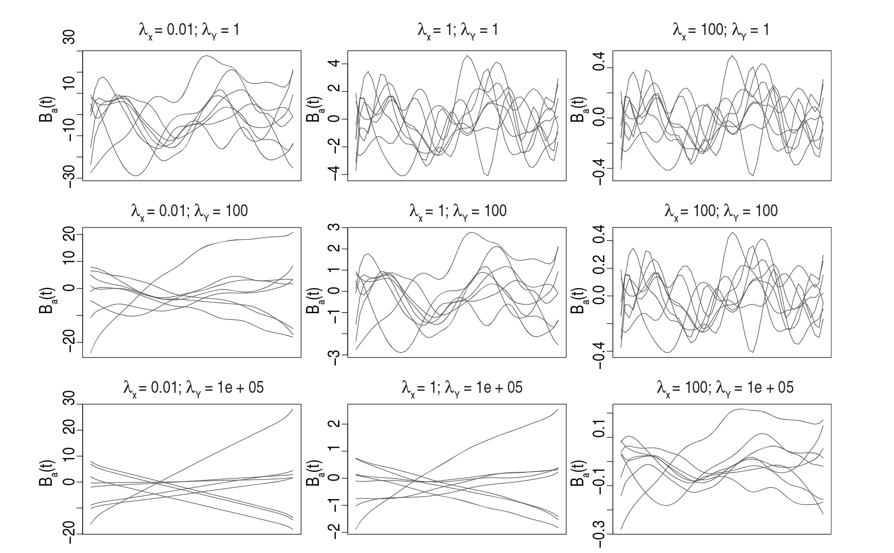


While the discussion paper describes model terms with a single smoothing parameter in t direction, locally varying smoothness is possible in our framework as well. Essentially, the smoothing parameter is then itself allowed to be a smooth function along t (Wood, 2011, Section 5.1). Such locally adaptive smoothing is feasible for all model terms in the general model (2.1) of the main article using
There seems to be a misunderstanding regarding the degrees of freedom for the individual model terms in the gradient boosting approach. It is correct that the degrees of freedom of all base learners in a given model are set to a common (low) number in order to achieve unbiased selection of baselearners (cf. Hofner et al., 2012). Nevertheless, the estimated functions adapt to the complexity of the underlying effects over the iterations: baselearners for model terms requiring more flexibility will be more frequently selected and updated, thereby adaptively increasing the effective degrees of freedom of the respective model term. This also proved true in our simulations when looking at anisotropic effect surfaces, which seem to concern both Paul Eilers and Jeff Morris: While the smoothing parameters for bivariate terms are chosen such that the base learner has a given number of degrees of freedom, for example, by choosing a single smoothing parameter
Jeff Morris asks about the assumed error term structure, and he and Anna Maria Paganoni and Laura Sangalli (PS) raise the issue of dependent functional data. While we do not specify a smooth residual curve
As another important aspect, we would like to point out that in the proposed general model formulation, we cover many other loss functions and response distributions as well as GAMLSS in addition to Gaussian, t- or quantile regression, which we see as an advantage compared to most competing approaches. This is also illustrated in our application in the main article with a beta regression with or without modelling of the conditional variance. Additional response distributions can now be added fairly easily even for the mixed model-based approach (see Wood and Fasiolo, 2016), while the boosting-based approach for GAMLSS we build on (Hofner et al., 2014) already implements all of the response distributions described in Stasinopoulos and Rigby (2007, Section 1.3).
María Durban and Carmen Aguilera-Morillo (DM) raise some issues with regard to the estimation and choice of basis and penalty for the functional random effects. As our approach is completely indifferent towards the estimation method used for the FPC basis of the functional random effects, it would also be possible to use it with FPCs estimated using Aguilera and Aguilera-Morillo (2013). However, it is unclear to us how to extend the required presmoothing step to sparse or irregular functional data or non-i.i.d. data with more complicated grouping structure along the lines of Cederbaum et al. (2016). We would also like to point out that the comparison of the proportion of variability explained (PVE) they present (their Table 1) is somewhat misleading, as the denominator in the PVE (i.e., the total variability of the input data) is smaller for the heavily presmoothed residual curves they use than for the raw residuals we use. When we repeat the analysis for DM's Table 1 with data presmoothed with 80 instead of the 20 B-spline basis functions DM used (proportion of raw variability ‘lost to smoothing’: 0.05% and 2.2%, respectively), the differences between the two approaches mentioned by DM practically disappear (cf. Table 1 and Figure 2).
Percentage of variability explained by first eight FPCs estimated via smoothed covariance on raw residuals (I, top) and penalized FPCA (Aguilera and Aguilera-Morillo, 2013) on presmoothed residuals represented with 80 B-splines (II, bottom).

First two eigenfunctions estimated via smoothed covariance on raw residuals (dashed red) and penalized FPCA (Aguilera and Aguilera-Morillo, 2013) on presmoothed residuals represented with 80 B-splines (solid black).

Plot of raw residuals
(black, solid) after estimation of mean structure and centring (model without smooth residuals/functional random effects) and estimated pffr functional random effects
using the first 20 FPCs (solid green) or 20 cubic B-spline basis functions (dashed blue) as well as DM's method using 23 cubic B-spline basis functions for
(dotted red).
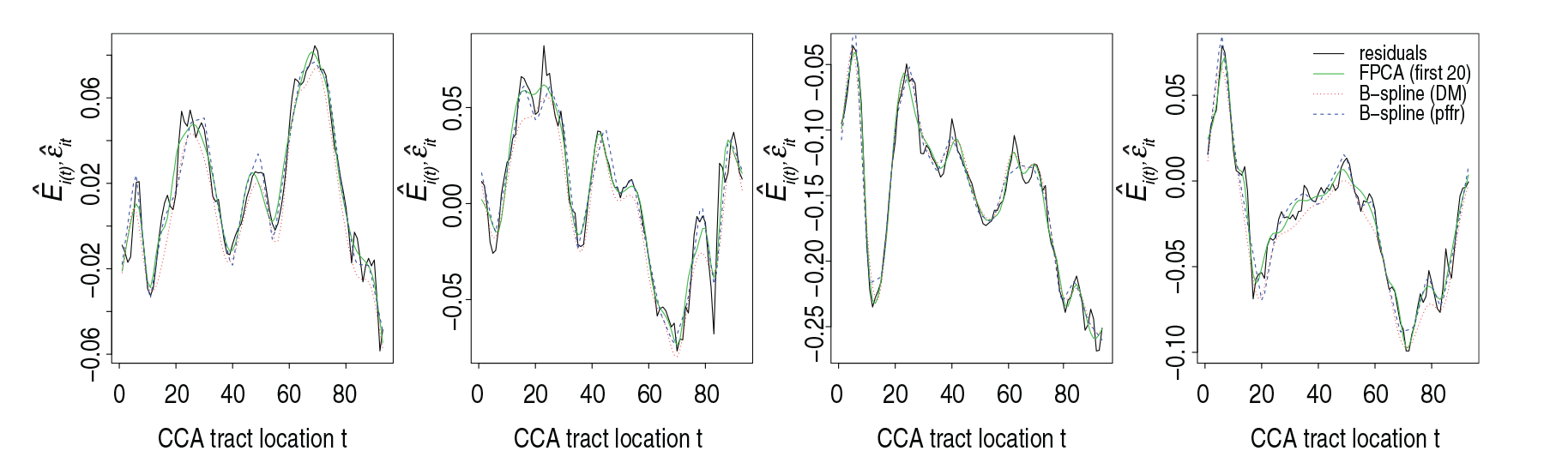
We are grateful to DM for pointing out that we chose an insufficiently flexible basis for the functional random effects in the main article (cf. their Figure 2). However, this should not be construed as a defect of the method itself, but rather as a question of (sub-optimal) model specification. Re-estimating the model with functional random effects based on 20 instead of 8 FPCs or alternatively 20 B-spline basis functions per subject, we achieve results that are very similar to those achieved with the 23 B-spline basis functions per subject used by DM. These results are shown in Figure 3.
Regarding the alternative penalty structure that DM give in their equations (3.2) and (3.3), we would like to point out that this single smoothing parameter penalty does not regularize the components of the random effect curves that are unpenalized by their roughness penalty
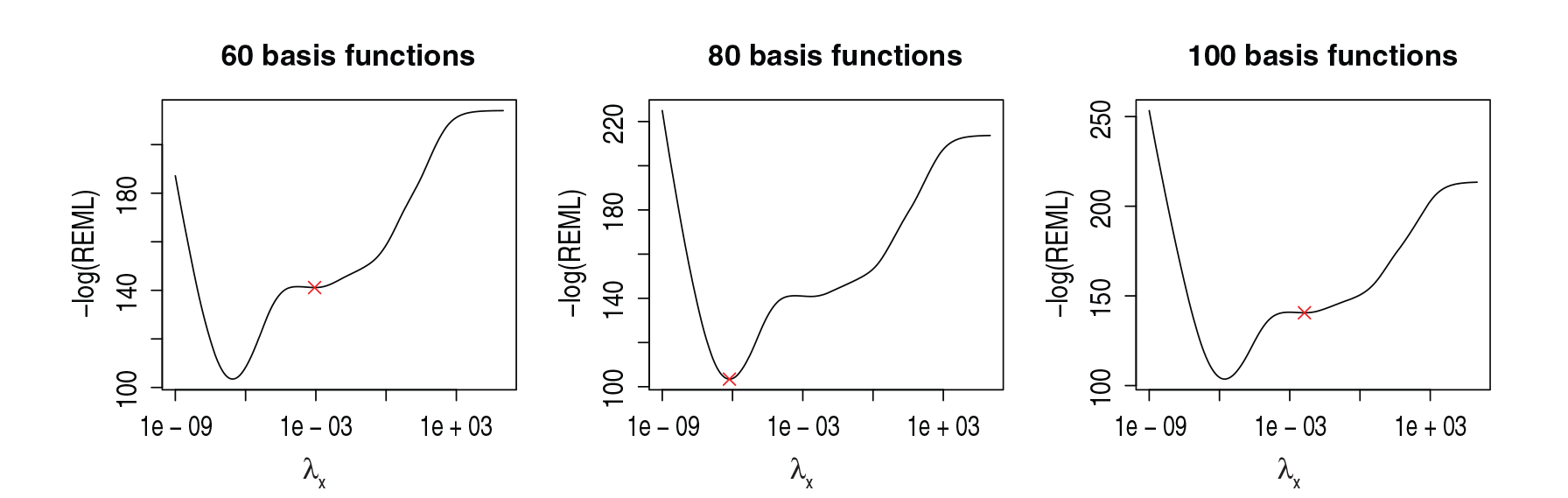
Plot of negative log REML criterion as a function of smoothing parameter
for the penalized signal regression of water content of fossil fuels with different basis sizes. REML estimates of
returned by mgcv are marked with red crosses.
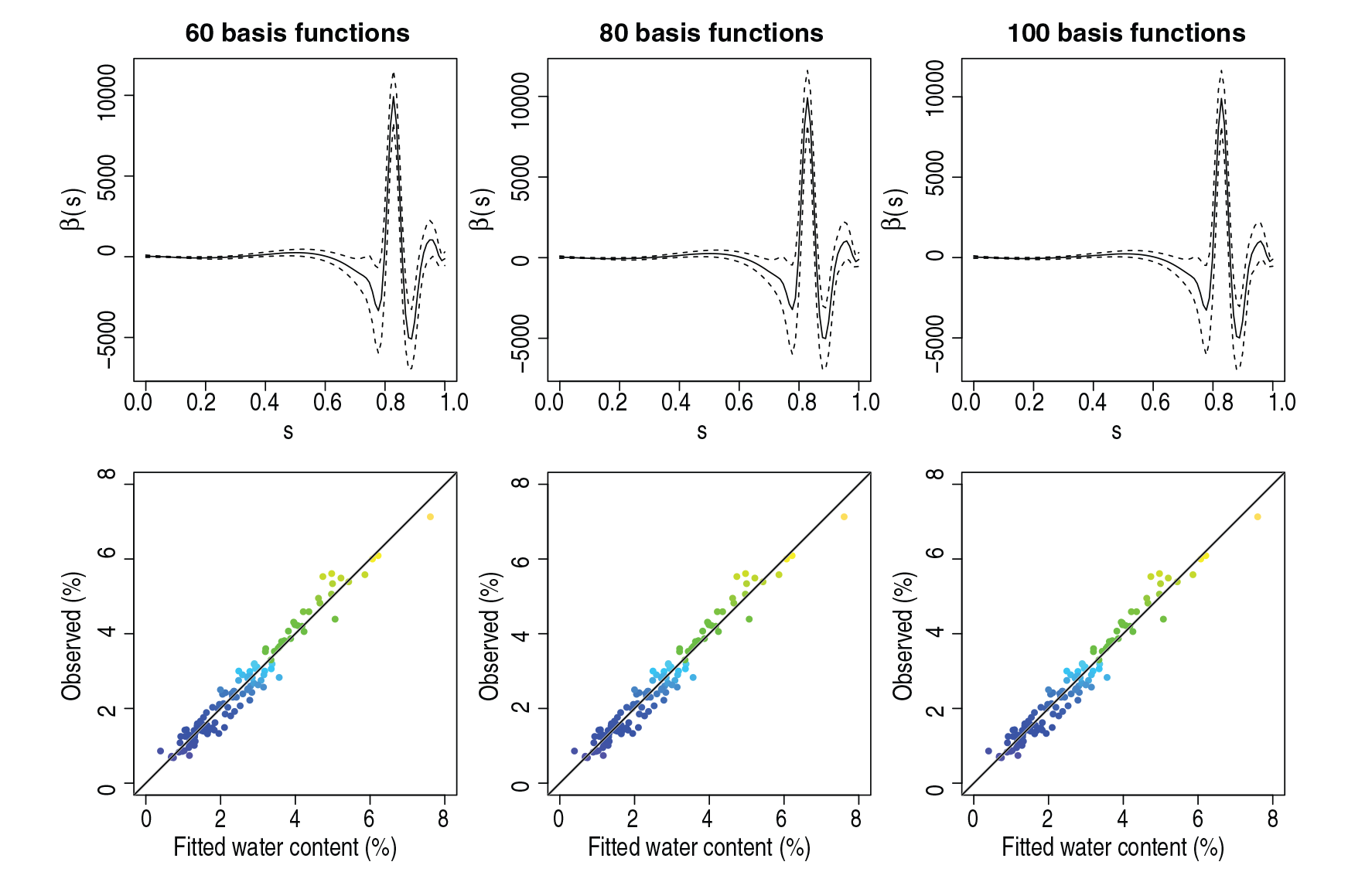
Adaptive spline fits (cubic B-splines, second-order difference penalty) for penalized signal regression of water content of fossil fuels with different basis sizes. Top row: estimated coefficient functions. Bottom row: observed versus fitted values.
Paul Eilers points out that the default settings of
Many of the discussants are concerned about neglected sources of estimation uncertainty and methods for properly accounting for the complicated covariance structures typical of functional datasets, as well as testing, model choice and variable selection.
The contribution of Piotr Kokoszka and Mathew Reimherr (KR) raises the important issue of how to properly account for intra-functional autocorrelation and showcases some valuable tools for constructing confidence intervals that take into account the autocorrelation of residual curves. However, we strongly disagree with their broad conclusion that ‘estimates produced by
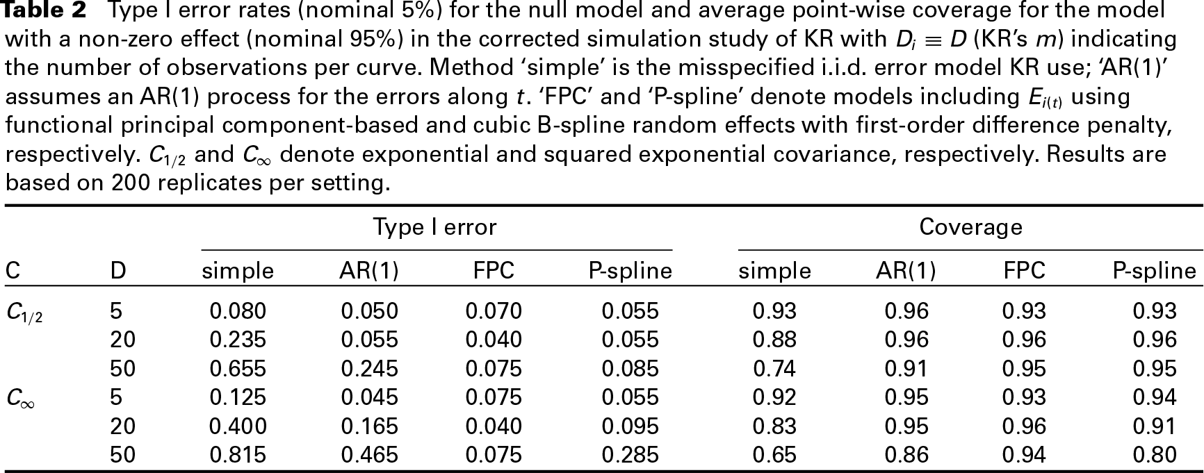
To more fairly evaluate the severity of the issue KR raise, we repeat their simulation study with an error process that includes an i.i.d. component in addition to a smooth auto correlated process of roughly the same variability while taking advantage of
Type I error rates (nominal 5%) for the null model and average point-wise coverage for the model with a non-zero effect (nominal 95%) in the corrected simulation study of KR with
(KR's m) indicating the number of observations per curve. Method ‘simple’ is the misspecified i.i.d. error model KR use; ‘AR(1)’ assumes an AR(1) process for the errors along t. ‘FPC’ and ‘P-spline’ denote models including
using functional principal component-based and cubic B-spline random effects with first-order difference penalty, respectively.
and
denote exponential and squared exponential covariance, respectively. Results are based on 200 replicates per setting.
In his excellent contribution contrasting his functional mixed model (FMM) and our approach, Morris states that any inference conditional on subject-specific random effects ‘would not account for the subject-to-subject variability [...] and the model would not effectively make inference on the population from which the subjects were drawn’ (Section 2.3). This is a rather more subtle issue. First, Morris's statement should not be interpreted to mean that conditional models ignore inter-subject variability which they model explicitly, merely that the focus of inference is different. For illustration, let us focus on a simple Gaussian linear mixed model
Jiawei Bai, Andrada Ivanescu and Ciprian Crainiceanu (BaIC) list some proposed tests for functional regression methods and bemoan the lack of a general and validated implementation of tests in functional regression, and KR and Morris raise the important objection that inference for functional effects often calls for simultaneous (or regional) confidence intervals and tests. In this context, it is worth noting that our mixed model-based framework—in addition to point-wise tests based on Wood et al. (2016b)—does offer simultaneous tests of effects based on Wood (2013a,b). Simultaneous confidence bands could be constructed along the lines of Ruppert et al. (2003, Section 6.5), similar to what the Morris group used for simultaneous credible bands in Meyer et al. (2015); alternatively, KR show reliable (albeit conservative) performance of their joint CIs even for their heavily misspecified model. Of course, these frequentist-penalized approaches will never be as flexible and easily customizable as Bayesian inference where the full posterior is available as for Morris et al.’s FMM.
In terms of model choice, the mixed model-based framework offers a generally applicable corrected conditional AIC that also incorporates smoothing parameter uncertainty (Wood et al., 2016b, Section 5) and can be used to select or deselect any terms in the model as well as to compare say smooth vs. linear or constant specifications. Model term selection for generalized additive mixed models based on full-rank penalties has alternatively been proposed in Marra and Wood (2011). For term selection in our boosting-based approach, we use cross-validated ‘early stopping’ of boosting iterations (Bühlmann and Hothorn, 2007) and stability selection (Meinshausen and Bühlmann, 2010; Shah and Samworth, 2013), which is theoretically well founded with strong guarantees on error rates.
Jeff Morris, Paul Eilers, BaIC and DM raise some interesting issues with regard to the actual implementations of the model class we present. We are looking forward to the implementation of the separation of overlapping penalties (SOP) algorithm combined with generalized linear array models (GLAM) representation announced by DM, which has the potential for large reductions in computing time and memory requirements. Unfortunately, they were unable to share working code with us for the preparation of this rejoinder for a more detailed comparison. As we describe in the article, the GLAM arithmetic implemented in our boosting-based approach will only ever be feasible for functional responses sampled on a common grid (with potential missings) and for the subset of model terms in which the marginal basis functions over
The sweep-operator trick (Goodnight, 1978; Herrick and Morris, 2006), used in
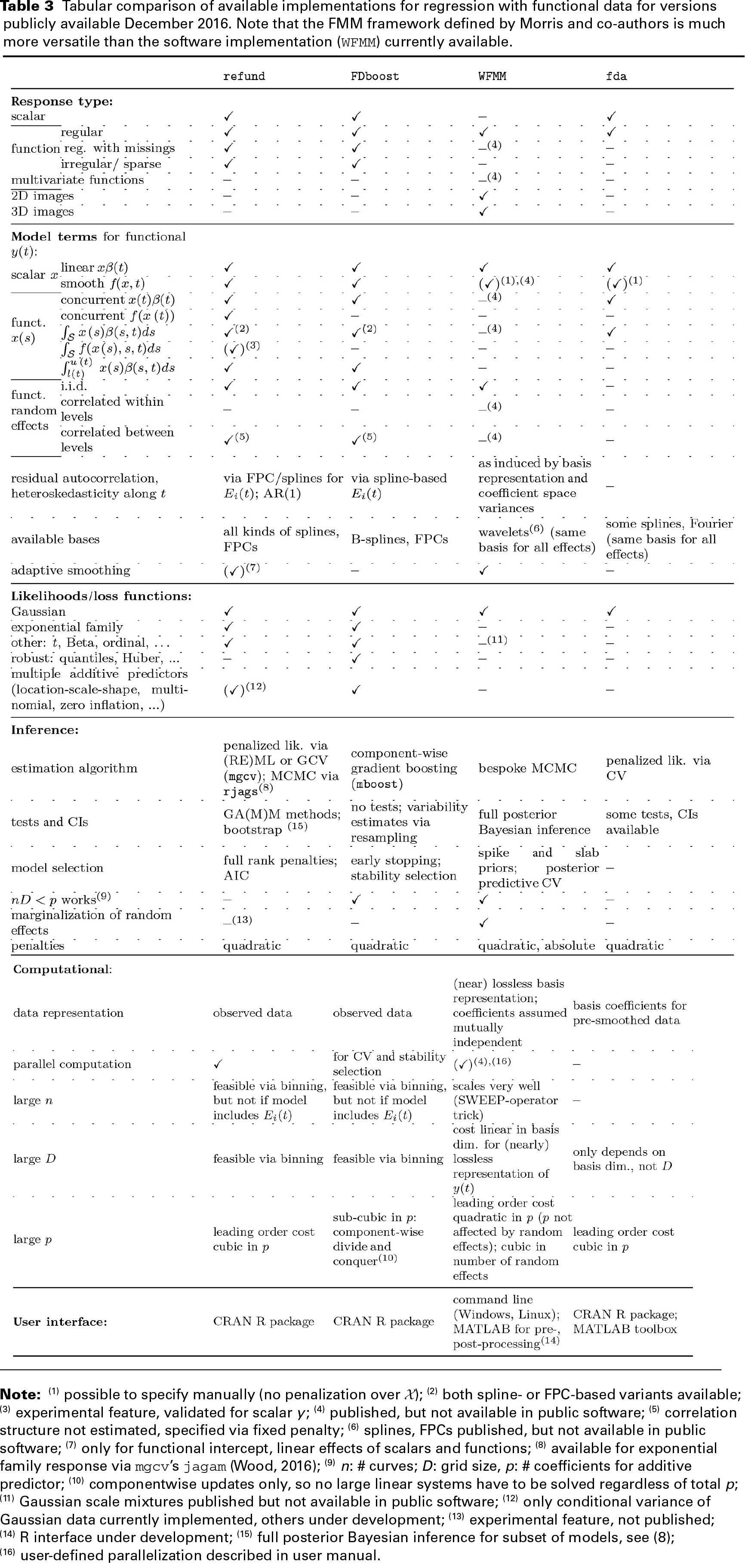
Tabular comparison of available implementations for regression with functional data for versions publicly available December 2016. Note that the FMM framework defined by Morris and co-authors is much more versatile than the software implementation (WFMM ) currently available.
Tabular comparison of available implementations for regression with functional data for versions publicly available December 2016. Note that the FMM framework defined by Morris and co-authors is much more versatile than the software implementation (WFMM ) currently available.
As suggested by BaIC, Table 3 represents our best effort to summarize the current capabilities of the four most mature implementations of regression models for functional data that we are aware of. Of course, many other software solutions offering more specialized routines for certain tasks are available (cf. the implementations mentioned in Section 1.4 of the main article). Note that the section ‘model terms’ in the table does not describe the scope of implemented interaction effects for reasons of space. We are looking forward to the planned comprehensive R implementation of Morris et al.’s FMM framework, which will fill further cells in the table and mean that the full flexibility of their developed framework will be publicly available.
Outlook and open questions
Regardless of the efficacy of random-effect-based approaches for dealing with intra-functional autocorrelation and achieving well-calibrated inference, Jeff Morris correctly points out the heavy computational cost of this conditional modelling strategy which does not scale well for datasets with more than a couple of hundred functional observations. At least for Gaussian functional data, an extension of our conditional modelling strategy by including an estimated marginal intra-functional covariance structure, possibly along the lines of the penalized GEE approach of Wang et al. (2013), would be an important addition to the framework presented here. An implementation of this idea is under development in the form of the prefer a marginal model approach instead of a conditional one for the autocovariance structure of functional residuals, at least for Gaussian data, perform (nearly) lossless compression of functional responses as an optional pre-processing step to make time and memory requirements (more) independent of grid lengths, use GLAM arithmetic for model terms where possible, use the sweep-operator trick for (iteratively reweighted) least squares (IW)LS-like estimation steps where possible, discretize or bin covariates in large data sets and use the resulting compact representation of associated basis matrices, use sparse matrix representations of basis matrices and penalties, where possible.
Note, however, that many of these algorithmic improvements will not be trivial or even feasible for sparse or irregular data.
On the subject of functional covariates, we agree with Paul Eilers that ‘Many quite different coefficient curves can give essentially identical fitted values or predictions of the dependent variable’. This is due to the high number of function grid points that are used as covariates compared to the number of observations and to their high collinearity. In the main article and Scheipl and Greven (2016), we have discussed the resulting identifiability issue and the inherently important role of assumptions like the coefficient function β being smooth or being in the span of the first few eigenfunctions of a functional covariate. However, we do not agree that only prediction performance matters. This is certainly of interest in almost all applications, but there is also often legitimate interest in β itself. Also, if we do out of sample prediction on completely new data, say on fossil fuel samples from a different country, where the functional covariate is somewhat different, predictions might differ depending on β. For example, functions that were approximately orthogonal to the original functional covariates and thus could be added with an arbitrary constant to β without changing an unpenalized fit, might be no longer orthogonal, and the arbitrary constant can now strongly change the model predictions. If the assumptions implied by the penalty are reasonable, then this may constitute an advantage of penalized spline-based approaches over FPC-based approaches, as the latter are completely determined by the given dataset.
We also welcome the discussions by PS, BaIC and others on important future directions in functional data analysis, which excellently complement our own outlook by further important areas of research that the community should tackle in the coming years. Regarding the topics of dimension reduction and spatio-temporal processes/imaging data, we have worked on multivariate functional principal component analysis (FPCA) approaches for dimension reduction that can jointly tackle imaging and functional data (Happ and Greven, 2016) and will strive to include this approach into our general modelling framework. With respect to the relative sparsity of Bayesian methods that BaIC point out, we agree that it would be a valuable addition to have a wider range of Bayesian functional regression models available. We have, in fact, started implementing a flexible class of Bayesian models for another area of interest that BaIC identify, namely joint models for longitudinal (sparse functional) and time to event data (see Köhler et al., 2016). This is based on the R package
In conclusion, we believe that regression models for functional data remain an exciting and active area of research, where much has been achieved and much needs to be done in order to develop suitable methods for the complex functional datasets of today.
Footnotes
Acknowledgments
Financial support was provided by the German Research Foundation (DFG) through Emmy Noether grant GR 3793/1-1.