Subject-specific modelling of paired comparison data: A lasso-type penalty approach

Abstract

In traditional paired comparison models heterogeneity in the population is simply ignored and it is assumed that all persons or subjects have the same preference structure. In the models considered here the preference of an object over another object is explicitly modelled as depending on subject-specific covariates, therefore allowing for heterogeneity in the population. Since by construction the models contain a large number of parameters we propose to use penalized estimation procedures to obtain estimates of the parameters. The used regularized estimation approach penalizes the differences between the parameters corresponding to single covariates. It enforces variable selection and allows to find clusters of objects with respect to covariates. We consider simple binary but also ordinal paired comparisons models. The method is applied to data from a pre-election study from Germany.

Keywords

BTLLasso Paired comparison Bradley-Terry-Luce model lasso heterogeneity

1 Introduction

Paired comparison is a well established method to measure the relative preference or dominance of objects or items. The aim is to find the underlying preference scale by presenting the objects in pairs. The method has been used in various areas, for example, in psychology, to measure the intensity or attractiveness of stimuli, in marketing, to evaluate the attractiveness of brands, in social sciences, to investigate value orientation (e.g., Francis et al., 2002). In all these applications the objects or stimuli are presented in an experiment. But paired comparisons are also found in sports whenever two players or teams compete in a tournament. Then the non-observable scale to be found refers to the strengths of the competitors. Paired comparisons can also be obtained from ranked data (Francis et al., 2002) or from rating scale data (Dittrich et al., 2007). In this kind of data, respondents rank a predefined number of objects or assign values from a Likert scale to the objects, always referring to a certain attitude of the respondents towards the objects. Building differences between the ranks or rating scales yields (binary or ordered) paired comparison data. We consider an application that shows how to analyse rating scales for the preference of parties by paired comparisons. In a German pre-election study the respondents were asked to scale the most well-known German parties. The focus of the analysis is on the inclusion of subject-specific covariates to account for the heterogeneity in the population and to investigate which variables determine the preference. More precisely, we investigate which clusters of parties are distinguished by specific covariates allowing that some covariates have no effect on the preference at all.

The most widely used model for paired comparison data is the Bradley-Terry-Luce (BTL) model. It has been proposed by Bradley and Terry (1952) and is strongly linked to Luce's choice axiom (Luce, 1959). The basic model has been extended in various ways allowing for dependencies among responses, time dependence or simultaneous ranking with respect to more than one attribute. Overviews are found in the review of Bradley (1976), the monograph of David (1988) and more recently in the review of Cattelan (2012). The method proposed in this work can be applied both to binary and ordered response. Former approaches for ordered responses in paired comparisons include Tutz (1986) and Agresti (1992). Dittrich et al. (2004) combine ordered responses and the inclusion of covariates within a log-linear model framework that uses the Poisson-multinomial equivalence.

In traditional paired comparison models it is assumed that the strengths of the objects are fixed and equal for all subjects. Early versions of the explicit modelling of heterogeneity by including subject-specific covariates were given by Tutz (1989) and Dittrich et al. (1998). Various models with subject-specific covariates have been considered since then, see Dittrich et al. (2000), Francis et al. (2002), Hatzinger et al. (2009), Dittrich et al. (2007), Francis et al. (2010), Turner and Firth (2012) and Francis et al. (2014). Software has been provided by Hatzinger and Dittrich (2012). When introducing subject-specific variables, the main problem is the large number of parameters that has to be estimated. Therefore, it is important to keep the dimensionality of the model as low as possible. One way to obtain a smaller model is to use only those covariates that are needed. Variable selection methods, which are based on information criteria such as Akaike information criterion (AIC) and Bayesian information criterion (BIC) have been used by Dittrich et al. (2000), Francis et al. (2002), Francis et al. (2010). More recently, Casalicchio et al. (2015) presented a boosting approach that is able to select explanatory variables. A quite different approach has been proposed by Strobl et al. (2011). It is based on recursive partitioning techniques (also known as trees) and automatically selects the relevant variables among a potentially large set of variables. The method proposed here is an alternative to handle the inherently high dimensional estimation problem that comes with the inclusion of explanatory variables. Maximum likelihood (ML) estimation is replaced by penalized estimation methods. By using a specific lasso-type penalty, the method is able to form clusters of objects that share the same effect of the explanatory variables which generate heterogeneity.

In Section 2 the basic BTL model for binary and ordered response is introduced. Then the model is extended to include subject-specific covariates. Section 3 contains the integration of the proposed model into the framework of generalized linear models (GLMs) and the penalty term is introduced. Section 3 also describes the implementation of the algorithm, the search for the optimal tuning parameter and the calculation of bootstrap confidence intervals. In Section 4, the method is applied to data from the German Longitudinal Election Study (GLES).

2 Bradley-Terry models with covariates

2.1 The basic model

Let ${a_{1}, \dots, a_{m}}$ denote the set of objects or items to be compared in a paired comparison experiment. The basic Bradley-Terry model (Bradley and Terry, 1952) specifies the probability that object $a_{r}$ is preferred over $a_{s}$ as

P (a_{r} ≻ a_{s}) = \frac{\exp (γ_{r} - γ_{s})}{1 + \exp (γ_{r} - γ_{s})},

where, for reasons of identifiability, we use the restriction

\sum_{r = 1}^{m} γ_{r} = 0

. The parameters

γ_{r}, r = 1, \dots, m

, represent the attractiveness of the objects

{a_{1}, \dots, a_{m}}

. The interpretation as strength parameters is straightforward. For

γ_{r} = γ_{s}

, the probability that

a_{r}

is preferred over

a_{s}

is 0.5, for growing distance

γ_{r} - γ_{s}

the probability increases.

With the random variable $Y_{(r, s)} = 1$ if $a_{r} ≻ a_{s}$ and $Y_{(r, s)} = 0$ otherwise one obtains the logit model

\log (\frac{P (Y_{(r, s)} = 1)}{P (Y_{(r, s)} = 0)}) = γ_{r} - γ_{s} .

2.2 Bradley-Terry models with ordered response

In some applications, paired comparison data can or should not be reduced to binary decisions. For example, in sport events like football matches where draws are also possible, simple binary paired comparisons are not appropriate. A model that allows for ordinal responses is the cumulative BTL model (Tutz, 1986; Agresti, 1992). It is an extension of the Rao-Kupper model for ties (Rao and Kupper, 1967), which has been widely used, see, for example, Dittrich et al. (2004) and Bockenholt (2001). The general model for $K$ response categories has the form

P (Y_{(r, s)} \leq k) = \frac{\exp (θ_{k} + γ_{r} - γ_{s})}{1 + \exp (θ_{k} + γ_{r} - γ_{s})}

(2.1)

with the same restriction

\sum_{r = 1}^{m} γ_{r} = 0

as in the binary model. The parameters

θ_{1}, \dots, θ_{K}

represent threshold parameters for the different levels of the response

Y_{(r, s)} ε {1, \dots, K}

. The response

Y_{(r, s)} = 1

corresponds to a strong preference of

a_{r}

over

a_{s}

and

Y_{(r, s)} = K

corresponds to a strong preference of

a_{s}

over

a_{r}

. The basic Bradley-Terry model can be seen as a special case of model (2.1) for binary response with

K = 2

The strength parameters $γ_{1}, \dots, γ_{m}$ have the same interpretation as in the binary model. With increasing $γ_{r}$ the probability for low response categories, and therefore the strong preference of $a_{r}$ over $a_{s}$ , increases while the probability for large response categories denoting dominance of $a_{s}$ decreases. The threshold parameters determine the preference for specific categories. The threshold for the last category $K$ is restricted to $θ_{K} = \infty$ so that $P (Y_{(r, s)} \leq K) = 1$ holds. Hence, there are only $K - 1$ free threshold parameters, but it is sensible to put further restrictions on the threshold parameters to ensure equal probabilities for corresponding categories if the order of the paired comparison is reversed. Therefore, we use the restrictions $θ_{k} = - θ_{K - k}$ and, if $K$ is even, additionally $θ_{K / 2} = 0$ . For example, if $K = 4$ only $θ_{1}$ is left as a free threshold parameter due to the restrictions $θ_{K} = \infty$ , $θ_{1} = - θ_{3}$ and $θ_{2} = 0$ . These restrictions ensure, for example, that $Y_{(r, s)} = 1$ (maximal preference of $a_{r}$ over $a_{s}$ ) has the same probability as $Y_{(s, r)} = K$ . Due to these restrictions, $⌊ \frac{K - 1}{2}$ (free) threshold parameters have to be estimated. In the special case of binary response ( $K = 2$ ) all threshold parameters are omitted and the model reduces to the ordinary Bradley-Terry model. If an order effect is required, for example to model the home advantage in sport competitions, an additional parameter can be included. For the application considered here no order effect is needed and, therefore, is omitted.

Formally, model (2.1) is a cumulative logit model, also called a proportional odds model. For a response variable consisting of $K$ ordered categories, one models $K - 1$ cumulative probabilities $P (Y_{(r, s)} \leq 1), \dots, P (Y_{(r, s)} \leq K - 1)$ . The probability for a single response category is represented by the difference $P (Y_{(r, s)} = k) = P (Y_{(r, s)} \leq k) - P (Y_{(r, s)} \leq k - 1)$ . Therefore, $P (Y_{(r, s)} \leq k)$ has to be greater or equal $P (Y_{(r, s)} \leq k - 1)$ for $k = 1, \dots, K$ to have non-negative probabilities for all single categories. As the probabilities only differ with respect to the threshold parameters, this is ensured if $θ_{1} \leq θ_{2} \leq \dots \leq θ_{K}$ .

2.3 Heterogeneity in the Bradley-Terry model

The models considered so far assume that all $n$ subjects have the same preference structure. Heterogeneity in the population is simply ignored. A more sensible assumption is that preferences depend on covariates that characterize the subject that chooses.

Let $Y_{i (r, s)}$ , $i = 1, \dots, n$ , denote the response of subject $i$ for given pair of objects $(a_{r}, a_{s})$ and $x_{i}^{T} = (x_{i 1}, \dots x_{ip})$ be a subject-specific covariate vector. It is assumed that the strength of the preference of object $a_{r}$ for subject $i$ is determined by $γ_{ir} = β_{r 0} + x_{i}^{T} β_{r}$ . That means there is a global strength parameter $β_{r 0}$ but the effective strength is modified by the covariates. The parameter $β_{r}^{T} = (β_{r 1}, \dots, β_{rp})$ contains the effect of the covariates on object $a_{r}$ . The corresponding model has the form

\begin{array}{l} P (Y_{i (r, s)} \leq k | x_{i}) = \frac{\exp (θ_{k} + γ_{i r} - γ_{i s})}{1 + \exp (θ_{k} + γ_{i r} - γ_{i s})} \\ = \frac{\exp (θ_{k} + (β_{r} 0 + x_{i} Τ β_{r}) - (β_{s} 0 + x_{i} Τ β_{s}))}{\begin{array}{l} 1 + \exp (θ_{k} + (β_{r} 0 + x_{i} β_{r}) - (β_{s} 0 + x_{i} β_{s})) \\ = \frac{\exp (θ_{k} + β_{r} 0 - β_{s} 0 + x_{i} Τ (β_{r} - β_{s}))}{1 + \exp (θ_{k} + β_{r} 0 - β_{s} 0 + x_{i} Τ (β_{r} - β_{s}))} \end{array}} \end{array}

(2.2)

As in model (2.1), the sum-to-zero constraints $\sum_{r = 1}^{m} β_{rj} = 0$ with $j = 0, 1, \dots, p$ are used for identifiability.

The model allows for different preference structures in sub-populations. For illustration, let us consider the simple case where the subject-specific variable codes a subgroup like gender, which has two possible values. Let $x_{i} = 1$ for males and $x_{i} = 0$ for females. Then the strengths parameters for object $a_{r}$ are

β_{r} 0 + β_{r} for males and β_{r} 0 for females .

The

β_{r}

represents the difference in attractiveness of object

a_{r}

between males and females. When objects

a_{r}

and

a_{s}

are compared the dominance in the male population is determined by

(β_{r 0} - β_{s 0}) + (β_{r} - β_{s})

, in the female population by

(β_{r 0} - β_{s 0})

. Thus the female population is like a reference population with dominance determined by the difference in the basic parameters

(β_{r 0} - β_{s 0})

. The preference in the male population is modified by the term

β_{r} - β_{s}

, and can be quite different.

In case of continuous variables like age in years, the interpretation is quite similar. Here, $β_{r}$ represents the change of the attractiveness of object $a_{r}$ when the age of the respondent increases by one year.

The model accounts for the heterogeneity in the population by explicitly linking the attractiveness of objects to explanatory variables. The object-specific parameters $β_{r}$ reflect how the attractiveness of an object $a_{r}$ depends on the covariates.

3 Penalized estimation

The main problem with the general model (2.2) is the number of parameters that are involved. One has (with the given restrictions) $⌊ \frac{K - 1}{2} ⌋$ threshold parameters and for each object the $(p + 1)$ -dimensional parameter vector $(β_{r 0}, β_{r})$ . In general, not all covariates might have a (different) influence on all $m$ objects. Therefore, we propose to use a penalized likelihood approach instead of ordinary ML estimation to reduce the number of involved parameters and to select the relevant variables. In the first step we embed the estimation into the framework of GLMs and then introduce penalty terms.

3.1 Embedding into generalized linear models

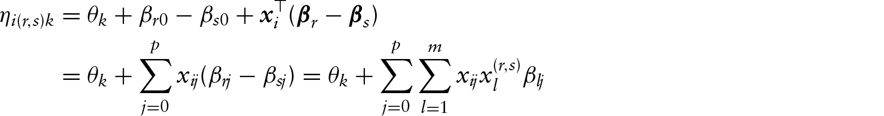
First, the ordinal Bradley-Terry model is embedded into the framework of GLMs. In the ordinal Bradley-Terry model without covariates the linear predictor $η_{(r, s) k} = θ_{k} + γ_{r} - γ_{s}$ can be given as

η_{(r, s) k} = θ_{k} + x_{1}^{(r, s)} γ 1 + … + x_{m}^{(r, s)} γ m = θ_{k} + (x^{(r, s)}) Τ γ,

where

x_{l}^{(r, s)} = 1

l = r

x_{l}^{(r, s)} = - 1

l = s

, and

x_{l}^{(r, s)} = 0

otherwise, encodes the considered pair. The whole vector

x^{(r, s)}

has the simple form

x^{(r, s)} = 1_{r} - 1_{s}

, where

1_{r} = (0, \dots, 0, 1, 0, \dots, 0)

has length

m

with 1 at position

r

. In this model, the strength of an object is the same for all subjects, which is a strong assumption ignoring potential heterogeneity.

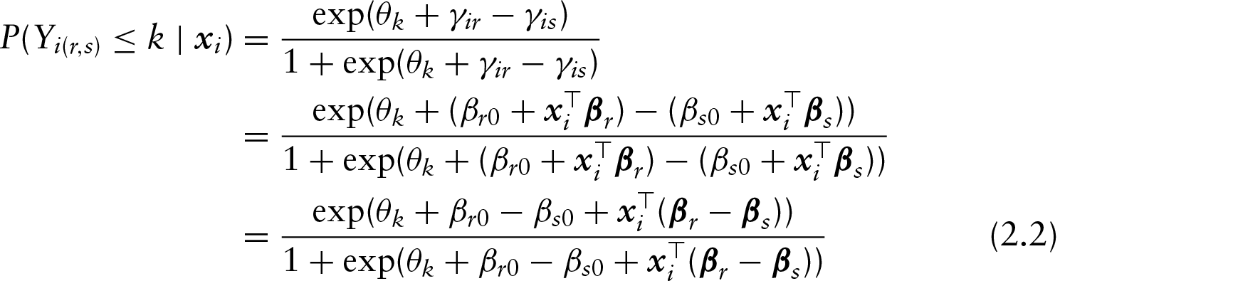
In the general model with covariates, and therefore explicit modelling of heterogeneity, the linear predictor has the form

\begin{array}{l} η_{i}_{(r, s) k} = θ_{k} + β_{r} 0 - β_{s} 0 + x_{i} Τ (β_{r} - β_{s}) \\ = θ_{k} + \sum_{j = 0}^{p} x_{i_{j}} (β_{r j} - β_{s_{j}}) = θ_{k} + \sum_{j = 0}^{p} \sum_{l = 1}^{m} x_{i j} x_{l}^{(r, s)} β_{l j} \end{array}

where

x_{i 0} = 1

is a fixed intercept. Here,

x i = (x_{i 1}, \dots, x_{ip})

represents a covariate vector associated to subject

i

and, therefore, the linear predictors for the same pair are different for subjects. For

j > 0

the predictor is determined by interactions between

x_{ij}

and the objects, which reflects the underlying structure that the object strength is modified by the covariates.

The link between the linear predictor and the probability $P (Y_{i (r, s)} \leq k \cdot x_{i})$ is determined by the logistic distribution function. It should be noted that the ordered response is transformed into a multivariate response $y i (r, s) = (y_{i (r, s) 1}, \dots, y_{i (r, s) q})$ with $q = K - 1$ binary variables where $y_{i (r, s) k} = 1$ if $Y_{i (r, s)} \leq k$ and $y_{i (r, s), k} = 0$ if $Y_{i (r, s)} > k$ . With $π_{i (r, s) k} = exp (η_{i (r, s) k}) / (1 + exp (η_{i (r, s) k}))$ , the covariance structure for such a multivariate response is given by

Cov (y_{i (r, s)}) = (\begin{array}{l} π_{i (r, s) 1} (1 - π_{i (r, s) 1}) π_{i (r, s) 1} (1 - π_{i (r, s) 2}) \dots π_{i (r, s) 1} (1 - π_{i (r, s) q}) \\ π_{i (r, s) 1} (1 - π_{i (r, s) 1}) π_{i (r, s) 2} (1 - π_{i (r, s) 2}) ⋮ \\ ⋮ ⋱ ⋮ \\ π_{i (r, s) 1} (1 - π_{i (r, s) q}) \dots \dots π_{i (r, s) 1} (1 - π_{i (r, s) q}) \end{array})

Because of the restrictions $θ_{k} = - θ_{K - k}$ and, if $K$ is even, $θ_{K / 2} = 0$ , the design matrix for the threshold parameters has a special form. As stated above, for a response with $K$ categories, $⌊ \frac{K - 1}{2} ⌋$ different threshold parameters have to be estimated. Therefore, the part of the design matrix corresponding to the paired comparison $(a_{r}, a_{s})$ of one subject is a $(K - 1) \otimes ⌊ \frac{K - 1}{2} ⌋$ matrix. This matrix is given by

(\begin{array}{l} 1 0 \dots 0 \\ 0 1 ⋮ \\ ⋮ ⋱ 0 \\ 0 \dots 0 1 \\ 0 \dots 0 - 1 \\ ⋮ ⋰ 0 \\ 0 - 1 ⋮ \\ - 1 0 \dots 0 \end{array}) o r (\begin{array}{l} 1 0 \dots 0 \\ 0 1 ⋮ \\ ⋮ ⋱ 0 \\ 0 \dots 0 1 \\ 0 \dots \dots 0 \\ 0 \dots 0 - 1 \\ ⋮ ⋰ 0 \\ 0 - 1 ⋮ \\ - 1 0 \dots 0 \end{array})

for K uneven or even, respectively. As stated above, for K = 2 the model reduces to a GLM with binomial distributed response and all threshold parameters are eliminated from the model.

3.2 Selection by penalization

In regression models with $ɑ$ as the parameter vector penalization approaches maximize the penalized likelihood

l_{p} (α) = l (α) - λ J (α),

where

l (ɑ)

is the usual log-likelihood and

J (ɑ)

is a penalty term that penalizes specific structures in the parameter vector. The parameter

λ

is a tuning parameter that specifies how seriously the penalty term has to be taken. A simple penalty term that could be used is the squared length of the parameter vector

J (ɑ) = ɑ ɑ = \sum ɑ_{i}^{2}

, known as ridge penalty (see, for example, Hoerl and Kennard, 1970; Nyquist, 1991; Segerstedt, 1992; LeCessie, 1992). Then, for

λ = 0

maximization yields the ML estimate. If

λ > 0

, one obtains parameters that are shrunk towards zero. For appropriately chosen

λ

the ridge estimator stabilizes estimates. A disadvantage of the ridge estimator is that it does not select variables. Thus no reduction of the model is obtained. An alternative penalty is the

L_{1}

-penalty, also known as the lasso (Tibshirani, 1996), which is able to select variables. Instead of the squared parameters one penalizes the absolute values of the parameters with the penalty term

J (ɑ) = \sum | ɑ_{i} |

. For penalized likelihood estimation, it is essential that all covariates are on comparable scales. Therefore, in the following it is assumed that all covariates are standardized.

However, the simple lasso cannot be used directly since penalty terms for paired comparison models have to account for the specific structure of the model. In particular, in model (2.2) one has the parameters of the regular (ordinal) BTL model, namely the threshold parameters and, for each object $a_{r}$ , a parameter $β_{r 0}$ for its basic attractiveness. They form the basic model and, therefore, will not be penalized. In the general model one has additional parameters for the interaction between the objects and the covariates. These parameters will be penalized to obtain the interactions that are actually needed. The proposed penalty term has the form

J (α) = \sum_{j = 1}^{p} \sum_{r < s} w_{r s j} \ β_{r j} - β_{s j} \,

where

r, s \in {1, \dots, m}

and the parameters are collected in

ɑ = (θ_{1}, \dots, θ_{K - 1}, β_{10}, \dots, β_{mp})

. Furthermore,

w_{rsj}

is a weight parameter constructed following the principle of adaptive lasso according to Zou (2006) and will be elaborated on at the end of this section.

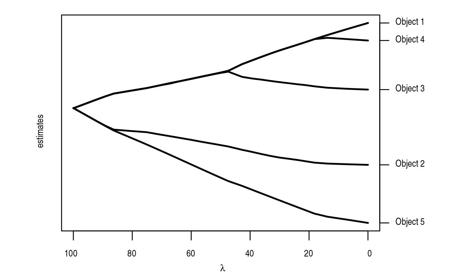
The penalty has the effect that the parameters referring to the same covariate are shrunk towards each other. For large values of $λ$ , the differences are shrunk to exactly zero so that the effect of a covariate is the same for two (or more objects). Therefore, the penalty yields clusters of objects which share the same effect of a certain covariate. As the tuning parameter grows, these clusters become bigger until all objects form one single cluster. In that case, due to the sum-to-zero constraints all parameters are zero and the covariate is irrelevant for the attractiveness of the objects. The penalty is a lasso-type fusion penalty rather than a simple lasso. Similar penalties have been used for the modelling of factors in GLMs by Bondell and Reich (2009), Gertheiss and Tutz (2010) and Oelker et al. (2014). More recently, penalties of this form have also been used in the modelling of paired comparison models, however, not for the modelling of heterogeneity by inclusion of covariates (Masarotto and Varin, 2012; Tutz and Schauberger, 2015).

For illustration, Figure 1 shows the coefficient paths corresponding to a covariate $j$ for a toy example with $m = 5$ objects.

Figure 1:

Exemplary coefficient paths for a covariate $j$ in a setting with $m = 5$ different objects along tuning parameter $λ$ (decreasing from left to right)

The paths are drawn along the tuning parameter

λ

, which is decreasing from left to right. It can be seen that the penalty enforces a clustering of the objects when the penalty is increased. In the unpenalized model, all objects form clusters of their own. With increasing penalty, objects 1 and 4 form a cluster, later object 3 is integrated into that cluster. Next, also objects 2 and 5 form a cluster and finally all objects form one single cluster. If all objects share the same parameter (all parameters are zero) that means that the respective covariate is eliminated from the model. Therefore, the proposed penalty term enforces both clustering of objects and variable selection at the same time.

Zou (2006) proposed the so-called adaptive lasso as an extension of the regular lasso. In contrast to regular lasso, it provides consistency in terms of variable selection. In the adaptive lasso, the single penalty terms are weighted with the inverses of the unpenalized ML estimates. In a similar way the weight parameters $w_{rsj}$ are defined by $w_{rsj} = | β_{rj}^{ML} - β_{sj}^{ML} |^{- 1}$ . The effect is that small differences in the ML estimates are penalized more strongly than bigger differences which additionally enforces the clustering of the parameters.

3.3 Implementation

Lasso penalized cumulative logit models have, for example, been used in Archer and Williams (2012) and are implemented for (R R Core Team, 2016) in Archer (2014a) and Archer (2014b). However, these implementations are limited to lasso penalties for coefficients. They cannot be used to penalize differences between parameters as required in the paired comparison case. Moreover, in order to obtain consistent estimates we want to include the weights $w_{rsj}$ . For that purpose, a new fitting algorithm was implemented that is able to fulfil these requirements. It is based on the idea of approximating penalties proposed by Oelker and Tutz (2015), which is implemented in the R-package gvcm.cat (Oelker, 2015), but not yet available for cumulative logit models. Following the suggestions of Fan and Li (2001), in Oelker and Tutz (2015) lasso or $L_{1}$ penalties are approximated by quadratic terms. Quadratic terms are differentiable and, therefore, can easily be incorporated in a (penalized) Fisher scoring algorithm. For shorter computation time, the fitting algorithm itself is implemented in C++ and integrated into R using the packages Rcpp (Eddelbuettel et al., 2011; Eddelbuettel, 2013) and RcppArmadillo (Eddelbuettel and Sanderson, 2014). The code is available on CRAN in the R-package BTLLasso (Schauberger, 2017).

3.4 Choice of penalty parameter

The performance of penalized estimation methods is essentially determined by the choice of the tuning parameter λ. It determines which covariates modify the attractiveness and form the clusters within the chosen covariates. Mostly, two different approaches are used to determine tunings parameters, namely model selection criteria and cross-validation. Model selection criteria like the AIC Akaike, 1973) or the BIC (Schwarz, 1978) try to find a compromise between the complexity of the model and the model fit. The complexity of a model is determined by its degrees of freedom. While for ML estimation, the degrees of freedom simply correspond to the number of parameters, the degrees of freedom for penalized likelihood approaches, in particular with a penalty applied on differences, are not straightforward. Therefore, we use cross-validation. In cross-validation, the data set is divided into a predefined number of subsets. Each subset is once used as a test data set while the remaining subsets serve as training data. The model is fitted (for a predefined grid of values for the tuning parameter $λ$ ) on the training data while the test data are used for prediction. Then the predictive performance in the test data can be measured, for example by using the deviance or the ranked probability score (RPS) (Gneiting and Raftery, 2007). For ordinal paired comparisons, the RPS is preferable as it uses the ordinal structure of the data while the deviance just uses multinomial scale level. The RPS can be denoted by

R P S (γ, \hat{π} (k)) = \sum_{k = 1}^{K} {(\hat{π} (k) - 1 (y \leq k))}^{2},

where

π (k)

represents the cumulative probability

π (k) = P (y \leq k)

. This procedure provides a measure of the predictive performance of the model for every value from the predefined grid of tuning parameters. The tuning parameter with the best performance is chosen.

3.5 Confidence intervals

In contrast to ML estimators, for estimators from penalized likelihood approaches one cannot use the information matrix to obtain standard errors or confidence intervals. Therefore, alternative techniques have to be used. We propose to use the bootstrap method for that purpose. The main idea of bootstrap is to replace an unkown distribution by the respective empirical distribution function. Then, for a predefined number of bootstrap iterations B, a subsample from the empirical distribution function is drawn. The proposed procedure is applied to the sampled data set, including the model selection using cross-validation. Therefore, the additional variance originating from the process of model selection is incorportated in the resulting confidence intervals. Finally, for every parameter bootstrap confidence intervals can be calculated using the empirical $ɑ / 2$ and $1 - ɑ / 2$ quantiles from the B bootstrap estimates for the respective parameter.

4 Application to pre-election data from Germany

The proposed method is applied to data from the GLES, (see Rattinger et al., 2014). The GLES is a long-term study of the German electoral process. It collects pre- and post-election data for several federal elections.

4.1 Data

The data we are using here originate from the pre-election survey for the German federal election in 2013. In this specific part of the study, 2003 persons were asked to rate the most important parties. Altogether, the survey covered seven different parties. In the following, we only consider the five (at that time point) most important parties, the smaller parties AfD (Alternative für Deutschland/Alternative for Germany) and the Pirate Party (Piratenpartei) were eliminated. Therefore, only the parties that actually entered the German parliament Bundestag, are taken into consideration. These are the CDU/CSU (Christlich Demokratische Union/Christian Democratic Union and Christlich-Soziale Union/Christian Social Union), the SPD (Sozialdemokratische Partei Deutschlands/Social Democratic Party of Germany), the Greens (Die Grünen), the Left Party (Linkspartei) and the FDP (Freie Demokratische Partei/Free Democratic Party). For the upcoming federal election, the participants rated the single parties on a discrete scale from $- 5$ to $+ 5$ (Likert scale with 11 categories). Plass et al. (2015) used the data in the context of modelling approaches for undecidedness. The rating scales $Z_{r}$ reflect the general opinions of the participants of party $r$ with $+ 5$ representing a very positive and $- 5$ representing a very negative opinion. The main goal of this application is to analyze which characteristics of the participants are connected to the preference of parties. For that purpose, we transformed the scale values into paired comparisons by building differences of scores. More precisely, for each participant, the differences between the ranks of all parties were calculated, ending up with ordered paired comparisons with values between $- 10$ and $10$ . The response was narrowed down to an ordered response with five categories. The data now represent paired comparisons between all parties measured on an ordered five-point scale:

\begin{array}{l} Z_{r} - Z_{s} \in {6, 10} | \to Y_{(r, s)} = 1 : ` I strongly prefer party r over party s’ \\ Z_{r} - Z_{s} \in {1, 5} \to Y_{(r, s)} = 2 : ` I slightly prefer party r over party s’ \\ Z_{r} - Z_{s} = 0 \to Y_{(r, s)} = 3 : ` I have equal opinions of parties r and s’ \\ Z_{r} - Z_{s} \in {- 5, - 1} \to Y_{{r, s}} = 4 : ` I slightly prefer party s over party r’ \\ Z_{r} - Z_{s} \in {- 10, - 6} \to Y_{{r, s}} = 5 : `I strongly prefer party s over party r’ \end{array}

The transformation of rating scales to ordered paired comparison data was proposed by Dittrich et al. (2007). They also describe in detail the advantages of the transformation for the analysis of rating scales. In particular, the use of categories of the Likert scale may vary over individuals. By considering the differences between parties, interpersonal incomparabilities do not matter anymore. Moreover, the alternative strategy, namely direct modelling of the Likert scales, calls for multivariate models. Since each person responds to all the items one should model all the responses simultaneously. Common multivariate regression methods, which assume a normally distributed response, cannot be recommended for ordinal responses. Alternative models are marginal models with an ordinal response structure by using generalized equations estimation methodology (see, for example, Miller et al., 1993; Fahrmeir and Pritscher, 1996; Heagerty and Zeger, 1996). However, for ordinal data they are hard to handle and no procedure to reduce the number of parameters seems available. More seriously, marginal models focus on the responses not the differences between them.

For the GLES study, only residents in the Federal Republic of Germany with German citizenship, a minimum age of 16 years and living in private households were eligible (Rattinger et al., 2014). In our analysis, only persons with a minimum age of 18 years (which is necessary to be entitled to vote in federal elections) are included. After eliminating all persons who rated less than two parties (because two parties are required to have at least one paired comparison for a person), the remaining data set contains $1 921$ participants with $18 919$ paired comparisons. Within the study, several characteristics of the participants are observed that possibly could affect the preference for the single parties. For our application, the following covariates are considered:

Age: age of participant in years

Gender (1: female; 0: male)

EastWest (1: East Germany/former GDR; 0: West Germany/former FRG)

PersEcon Personal economic situation (1: good or very good; 0: neither/nor, bad or very bad)

Abitur School leaving certificate (1: Abitur/A levels; 0: else)

Unemployment (1: currently unemployed; 0: else)

Church (1: Attendance in Church/Mosque/Synagogue/...: at least once a month; 0: else)

Migration: Are you a migrant/not German since birth? (1: yes; 0: no)

The age of the participants ranges from 18 years to 99 years. The variable EastWest refers to the current place of residence where all Berlin residents are assigned to East Germany. As mentioned before, it is necessary that all covariates are on comparable scales. Therefore, all variables have been standardized and centered before the analysis.

4.2 Results

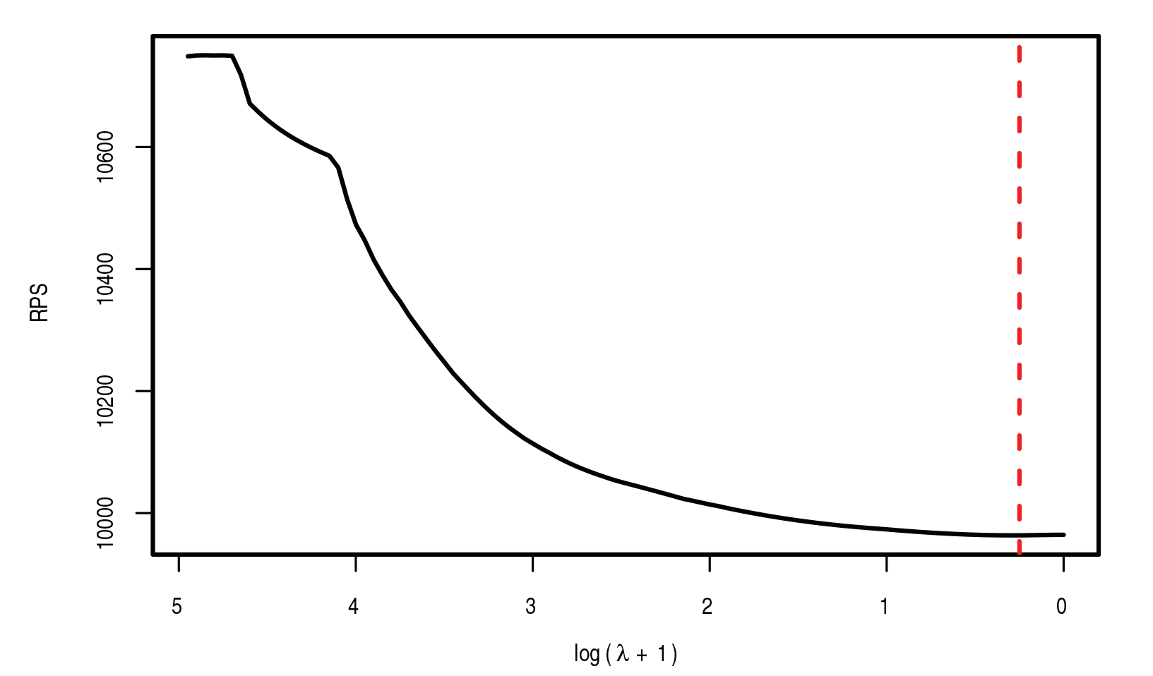
In the following, the results for the proposed method are presented for a model where all covariates described above are considered as possibly influential variables. The optimal model is determined by 10-fold cross-validation. Figure 2 shows the RPSs obtained by cross-validation plotted against $log (λ + 1)$ . The dashed vertical line represents the model with the lowest RPSs.

Figure 2:

RPS path for 10-fold cross-validation, dashed vertical line represents model with lowest deviance

Figure 3:

Coefficient paths for all unpenalized parameters (threshold parameters $θ_{1}$ and $θ_{2}$ and party-specific intercepts). Dashed vertical line represents optimal model according to 10-fold cross-validation

Figure 3 shows the corresponding coefficient paths for the threshold parameters

θ_{1}

and

θ_{2}

and the party-specific intercepts

β_{10}, \dots, β_{m 0}

. These parameters are not penalized. In principle, they might be different for different tuning parameters

λ

. In the current application, it is seen that both the threshold parameters and the intercepts hardly change along their paths.

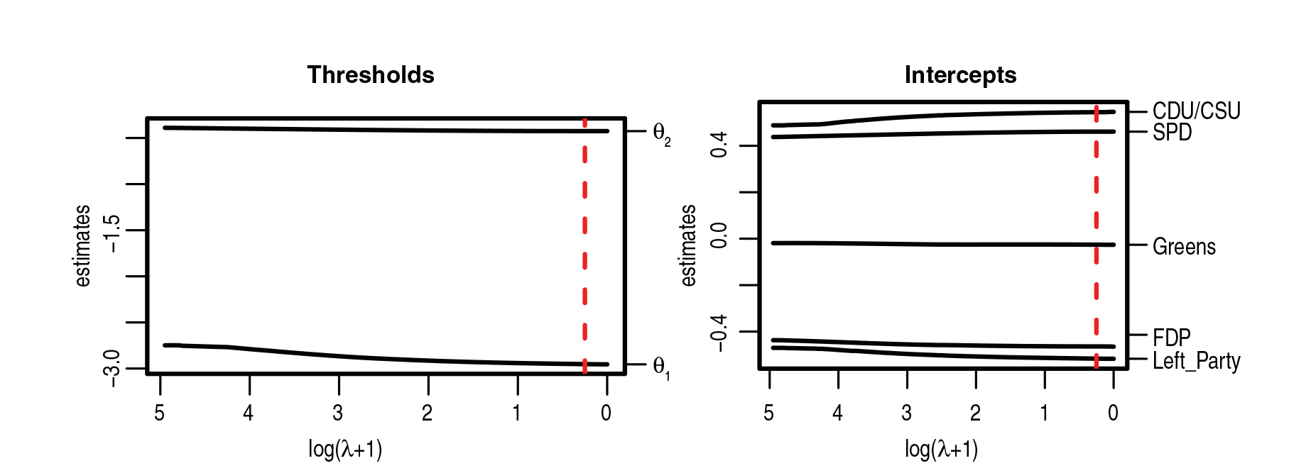
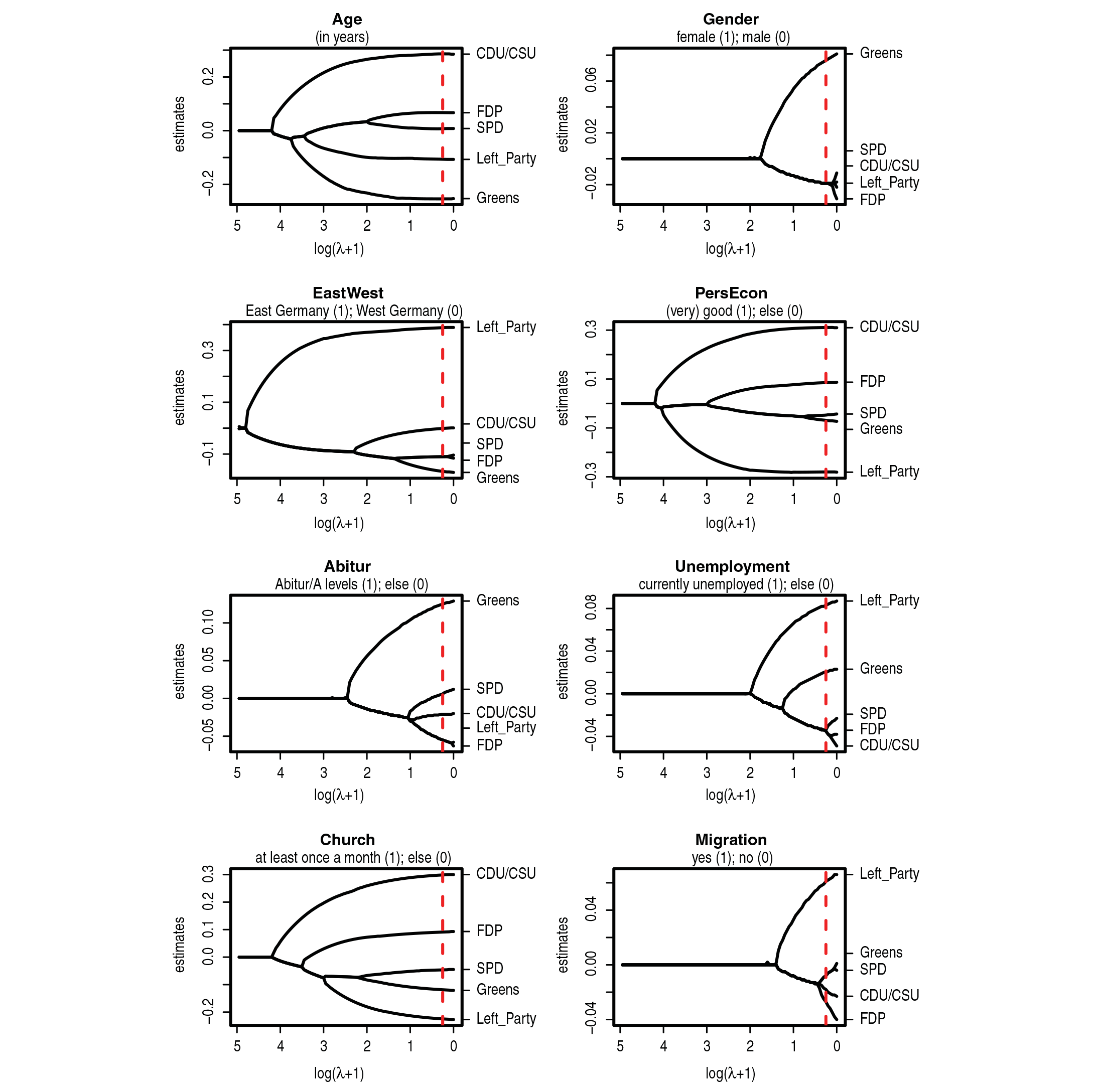
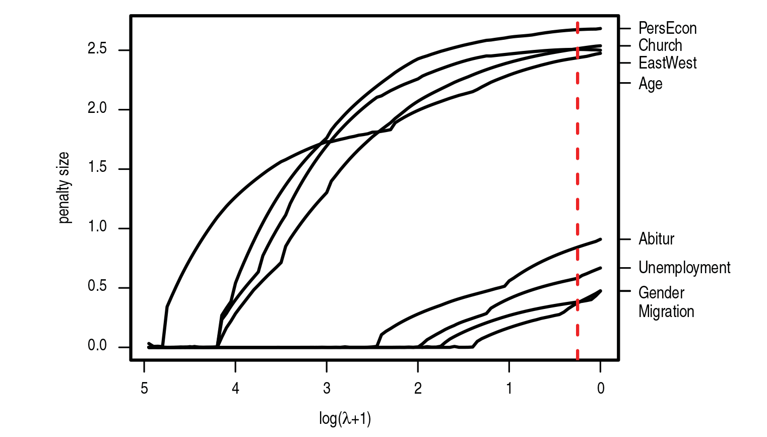
Figure 4 shows the corresponding coefficient paths for the eight covariates. The coefficient paths are drawn separately for each covariate. It is seen how the penalty term enforces clustering of the different parties. The dashed vertical lines represent the optimal model according to the 10-fold cross-validation.

The coefficient paths allow for interesting insights into how the preference of the voters for certain parties depends on characteristics of the voters themselves. Let us first consider the covariate unemployment. With respect to unemployment, the parties can be divided into three clusters. The Left Party and the Greens form single clusters while CDU, SPD and FDP form another cluster. As a global tendency one sees that unemployed persons tend to prefer the younger parties (Greens and Left Party) while the tendency to the more established parties (SPD, CDU, FDP) is reduced. For gender, only two different clusters are identified in the final model. The Greens are much more attractive to female than to male voters and form a cluster of their own. All remaining parties belong to a second cluster and are more attractive to male voters than to female voters. Also the variable Abitur has a very different effect for the Greens compared to all other parties confirming the reputation of the Greens to be a party attractive to those more highly educated. Overall, no variable is eliminated completely from the model, each variable has at least two clusters of parties. The variables age and church attendance have a specific impact on the preference of parties and every party forms a cluster of its own.

Figure 4:

Coefficient paths separately for all eight (scaled) covariates. Dashed vertical lines represent optimal model according to 10-fold cross-validation

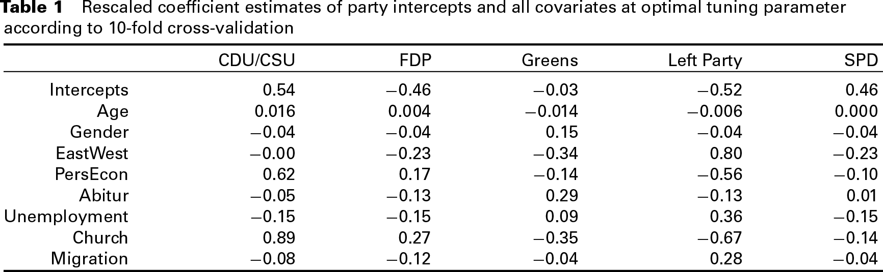
The resulting parameters (as estimated at the optimal tuning parameter according to the 10-fold cross-validation) are summarized in Table 1. In contrast to Figure 4, the coefficients have been rescaled so that they are interpretable with regard to the original scale of the variables. For example, when age is increased by 10 years, the attractiveness of the CDU/CSU increases by 0.16.

Table 1:

Rescaled coefficient estimates of party intercepts and all covariates at optimal tuning parameter according to 10-fold cross-validation

	CDU/CSU	FDP	Greens	Left Party	SPD
Intercepts	0.54	$-$ 0.46	$-$ 0.03	$-$ 0.52	0.46
Age	0.016	0.004	$-$ 0.014	$-$ 0.006	0.000
Gender	$-$ 0.04	$-$ 0.04	0.15	$-$ 0.04	$-$ 0.04
EastWest	$-$ 0.00	$-$ 0.23	$-$ 0.34	0.80	$-$ 0.23
PersEcon	0.62	0.17	$-$ 0.14	$-$ 0.56	$-$ 0.10
Abitur	$-$ 0.05	$-$ 0.13	0.29	$-$ 0.13	0.01
Unemployment	$-$ 0.15	$-$ 0.15	0.09	0.36	$-$ 0.15
Church	0.89	0.27	$-$ 0.35	$-$ 0.67	$-$ 0.14
Migration	$-$ 0.08	$-$ 0.12	$-$ 0.04	0.28	$-$ 0.04

Figure 5:

Paths representing the sums of absolute differences for the scaled parameters of all eight covariates. Dashed vertical line represents optimal model according to 10-fold cross-validation

Figure 5 shows the paths for whole covariates represented by the sum of absolute differences between all parameters corresponding to one covariate. Every covariate is represented by a single path. With the used penalty term, the sum of the absolute differences between all parameters corresponding to one covariate can be seen as a measure of effect strength for this covariate. Again, one has to keep in mind that all covariates have been standardized. It can be seen that, not very surprisingly, the personal economic situation of the voters is the most important modifier of the preference of a party in the data set. Yet, the first covariate that is included (for decreasing tuning parameter

λ

) is the covariate EastWest. Even 23 years after the German reunification, the differences between the former German Democratic Republic (GDR) and the former Federal Republic of Germany (FRG) were still extremely relevant in 2013. Also the covariates age and church attendance have very strong effects. Again, it can be seen that no variable is eliminated completely from the model. Figure 5 can provide valuable additional information on the paths depicted in Figure 4 where the variable importance is harder to recognize due to the different ranges in the single plots.

Figure 6:

Rescaled coefficient estimates and 95% bootstrap confidence intervals separately for all eight covariates

Finally, $B = 500$ bootstrap iterations were performed to receive confidence intervals. Figure 6 depicts the rescaled estimates of all (penalized) parameters together with the corresponding 95% bootstrap confidence intervals. It can be seen if two clusters differ distinctly from each other and how strongly the parameter estimates vary. The estimates for variables Age, EastWest, PersEcon and Church appear to be much less volatile than the estimates of the other variables. Both for Gender and Abitur, only the parameters for the Greens seems to differ substantially from the other parties.

4.3 Computation time

For illustration, in the following different computational times of the application are reported. The proposed method is implemented in the R-package BTLLasso (Schauberger, 2017) where also the data can be found. Both the cross-validation and the bootstrap-procedure can be sped-up by parallelization.

For the analysis, a computer with an Intel Xeon 2.60 GHz processor was used. As mentioned before, the data set contains $18 919$ paired comparisons with 5 possible response categories. The fitting of the model for a single fixed value of $λ$ takes about $12$ seconds, further values of $λ$ are faster as previous solutions can be used as starting values. The fitting of the model for the whole grid of 100 different values of $λ$ takes $6.1$ minutes. The cross-validation along the grid of 100 values of $λ$ was performed parallel on 10 cores. In total, the computation of the full $λ$ grid together with the cross-validation took $13.1$ minutes. For the bootstrap procedure, $B = 500$ bootstrap samples were drawn. The procedure was executed only on 40 values of the original $λ$ grid and was parallelized on 25 cores and took, in total, $11.1$ hours.

5 Concluding remarks

A method that reduces the dimensionality in ordered paired comparison model with subject-specific covariates is proposed. The developed feature selection approach utilizes penalization techniques with a specific lasso-type penalty. The penalty has two main features: First, the penalty clusters objects with regard to certain covariates. Therefore, one can identify clusters of objects whose preferences are equally affected by a covariate. Second, the penalty can eliminate whole covariates from the model indicating that the respective covariates do not affect the preference for one or another object (although in our application all variables had an effect on the preference). Bootstrap intervals can be calculated, which can be used to compare parameter estimates with respect to their variation.

In particular the ability to select and cluster distinguishes the method from the alternative approaches to model subject-specific effects. The methods that select variables by using information criteria, as considered, for example, by Dittrich et al. (2000), Francis et al. (2002) or Francis et al. (2010), exclude whole variables but do not identify clusters. The same holds for the boosting approach proposed by Casalicchio et al. (2015) because boosting methods are not designed to allow fusion of parameters. An additional advantage of penalty methods over boosting approaches is that the structure of the regularization is more clearly defined. In contrast to Strobl et al. (2011), where the underlying structure is searched for by recursive partitioning techniques, we consider a parametric model that allows for easy interpretation of parameters and clustering.

The proposed method could be extended in various ways. First, the restriction of the covariate effects to linear terms could be weakened by allowing for smooth covariate effects. A big challenge with such an approach would be to find an appropriate penalty term to have a similar cluster effect as for the linear terms. Second, the model could be extended by object-specific covariates similar to Tutz and Schauberger (2015). For the application to the data from the GLES in this work, this would correspond to the inclusion of party-specific covariates, for example the popularity of the respective leading candidates.

References

Agresti

(1992) Analysis of ordinal paired comp- arison data. Applied Statistics , 41, 287–97.

Akaike

(1973) Information theory and the extension of the maximum likelihood principle. In Petrov B and Caski F, eds. Second International Symposium on Infor- mation Theory , pages 267–81. Budapest: Akademia Kiado.

Archer

, Williams

AAA

(2012) L1 penalized continuation ratio models for ordinal respo- nse prediction using high-dimensional data- sets. Statistics in Medicine , 31, 1464–74. ISSN 1097-0258. \doi 10.1002/sim.4484. URL https://dx-doi-org.web.bisu.edu.cn/10.1002/sim.4484.

Archer

(2014a) Glmnetcr: Fit a penalized constrained continuation ratio model for predicting an ordinal response , R package version 1.0.2., URL http://CRAN.R-[project.org/package=glmnetcr].

Archer

(2014b) Glmpathcr: Fit a penalized continuation ratio model for predicting an ordinal response , R package version 1.0.3., URL http://CRAN.R-project.org/[package=glmpathcr].

Böckenholt

(2001) Thresholds and intransitiv- ities in pairwise judgments: A multilevel analysis. Journal of Educational and Behavioral Statistics , 26, 269–82.

Bondell

, Reich

(2009) Simultaneous factor selection and collapsing levels in anova. Biometrics , 65, 169–77.

Bradley

(1976) Science, statistics, and paired comparison. Biometrics , 32, 213–32.

Bradley

, Terry

(1952) Rank analysis of incomplete block designs, I: The method of pair comparisons. Biometrika , 39, 324–45.

10.

Casalicchio

, Tutz

, Schauberger

(2015) Subject-specific Bradley-Terry-Luce models with implicit variable selection. Statistical Modelling , 15, 526–47. doi 10.1177/ 1471082X15571817. URL http://smj.[sagepub.com/content/15/6/526.abstract] (last accessed 23 January 2017).

11.

Cattelan

(2012) Models for paired comparison data: A review with emphasis on dependent data. Statistical Science , 27, 412–33.

12.

David

(1988) The method of paired compari- sons, 2nd edition. Griffin's Statistical Mono- graphs and Courses 41. London: Griffin.

13.

Dittrich

, Hatzinger

, Katzenbeisser

(1998) Modelling the effect of subject- specific covariates in paired comparison studies with an application to university rankings. Applied Statistics , 47, 511–25.

14.

Dittrich

, Hatzinger

, Katzenbeisser

(2004) A log-linear approach for modelling ordinal paired comparison data on motives to start a PhD programme. Statistical Mode- lling , 4, 181–93. doi 10.1191/1471082X04 st072oa. URL http://smj.sagepub.com/[content/4/3/181.abstract].

15.

Dittrich

, Katzenbeisser

, Reisinger

(2000) The analysis of rank ordered prefere- nce data based on Bradley-Terry type models. OR-Spektrum , 22, 117–34.

16.

Dittrich

, Francis

, Hatzinger

, Katzen- beisser

(2007) A paired comparison app- roach for the analysis of sets of Likert-scale responses. Statistical Modelling , 7, 3–28. \doi 10.1177/1471082X0600700102. URL http://smj.sagepub.com/content/7/1/3.[abstract].

17.

Eddelbuettel

(2013) Seamless R and C++ integration with Rcpp . New York: Springer.

18.

Eddelbuettel

, Sanderson

(2014) Rcpparmadillo: Accelerating R with high- performance C++ linear algebra. Computa- tional Statistics and Data Analysis , 71, 1054–63. URL https://dx-doi-org.web.bisu.edu.cn/10.1016/[j.csda.2013.02.005] (last accessed 23 January 2017).

19.

Eddelbuettel

, François

, Allaire

, Chambers

, Bates

, Ushey

(2011) Rcpp: Seamless R and C++ integration. Journal of Statistical Software , 40, 1–18.

20.

Fahrmeir

, Pritscher

(1996) Regression analysis of forest damage by marginal models for correlated ordinal responses. Journal of Environmental and Ecological Statistics , 3, 257–68.

21.

Fan

, Li

(2001) Variable selection via nonconcave penalized likelihood and its oracle properties. Journal of the American Statistical Association , 96, 1348–60. \doi 10.1198/016214501753382273.

22.

Francis

, Dittrich

, Hatzinger

, Penn

(2002) Analysing partial ranks by using smoothed paired comparison methods: An investigation of value orientation in Europe. Journal of the Royal Statistical Society: Series C (Applied Statistics) , 51, 319–36.

23.

Francis

, Dittrich

, Hatzinger

(2010) Modeling heterogeneity in ranked responses by nonparametric maximum likelihood: How do Europeans get their scientific know- ledge? The Annals of Applied Statistics , 4, 2181–2202.

24.

Francis

, Dittrich

, Hatzinger

, Humphreys

(2014) A mixture model for longitudinal partially ranked data. Comm- unications in Statistics-Theory and Methods , 43, 722–34.

25.

Gertheiss

, Tutz

(2010) Sparse modeling of categorial explanatory variables. Annals of Applied Statistics , 4, 2150–80.

26.

Gneiting

Raftery

(2007) Strictly proper scoring rules, prediction, and estimation. Journal of the American Statistical Associa- tion , 102, 359–76.

27.

Hatzinger

, Dittrich

(2012) Prefmod: An R package for modeling preferences based on paired comparisons, rankings, or ratings. Journal of Statistical Software , 48, 1–31.

28.

Hatzinger

, Dittrich

, Salzberger

(2009) Präferenzanalyse mit R: Anwendungen aus marketing, behavioural finance und human resource management [Preference analysis in R: Applications from marketing, behavioural finance and human resource management]. Vienna: Facultas wuv.

29.

Heagerty

, Zeger

(1996) Marginal regres- sion models for clustered ordinal measure- ments. Journal of the American Statistical Association , 91, 1024–36.

30.

Hoerl

, Kennard

(1970) Ridge regression: Bias estimation for nonortho- gonal problems. Technometrics , 12, 55–67.

31.

LeCessie

(1992) Ridge estimators in logistic regression. Applied Statistics , 41, 191–201.

32.

Luce

(1959) Individual Choice Behaviour . New York: Wiley.

33.

Masarotto

, Varin

(2012) The ranking lasso and its application to sport tourna- ments. The Annals of Applied Statistics , 6, 1949–70.

34.

Miller

, Davis

, Landis

(1993) The analysis of longitudinal polytomous data: Generalized estimated equations and connections with weighted least squares. Biometrics , 49, 1033–44.

35.

Nyquist

(1991) Restricted estimation of genera- lized linear models. Applied Statistics , 40, 133–41.

36.

Oelker

M-R

(2015) Gvcm.cat: Regularized Cate- gorical Effects/Categorical Effect Modifiers/ Continuous/Smooth Effects in GLMs . R package version 1.9.

37.

Oelker

M-R

, Tutz

(2015) A uniform frame- work for the combination of penalties in generalized structured models. Advances in Data Analysis and Classification, page pub- lished online. ISSN 1862-5347. doi 10.1007/s11634-015-0205-y. URL https://dx-doi-org.web.bisu.edu.cn/10.1007/s11634-015-[0205-y] (last accessed 23 January 2017).

38.

Oelker

M-R

, Gertheiss

, Tutz

(2014) Regularization and model selection with categorical predictors and effect modifiers in generalized linear models. Statistical Modelling , 14, 157–77.

39.

Plass

, Fink

, Schöning

, Augustin

(2015) Statistical modelling in surveys without neglecting ≤the undecided’: Multinomial logistic regression models and imprecise classification trees under ontic data impre- cision—extended version (Technical Report 179). Germany: Department of Statistics, Ludwig-Maximilians-Universität München.

40.

R R Core Team (2016) R: A language and environ- ment for statistical computing . R Founda- tion for Statistical Computing, Vienna, Austria. URL http://www.R-project.org/.

41.

Rao

, Kupper

(1967) Ties in paired- comparison experiments: A generalization of the Bradley-Terry model. Journal of the American Statistical Association , 62, 194–204.

42.

Rattinger

, Roßteutscher

, Schmitt-Beck

, Weßels

, Wolf

(2014) Pre-election cross section (GLES 2013). GESIS Data Archive, Cologne, ZA5700 Data file Version 2.0.0.

43.

Schauberger

(2017) BTLLasso: Modelling het- erogeneity in paired comparison data , R package version 0.1-5, URL http://[CRAN.R-project.org/package=BTLLasso].

44.

Schwarz

(1978) Estimating the dimension of a model. Annals of Statistics , 6, 461–64.

45.

Segerstedt

(1992) On ordinary ridge regression in generalized linear models. Communica- tions in Statistics—Theory and Methods , 21, 2227–46.

46.

Strobl

, Wickelmaier

, Zeileis

(2011) Accounting for individual differences in Bradley-Terry models by means of recursive partitioning. Journal of Educational and Behavioral Statistics , 36, 135–53.

47.

Tibshirani

(1996) Regression shrinkage and selection via the lasso. Journal of the Royal Statistical Society , B 58, 267–88.

48.

Turner

, Firth

(2012) Bradley-Terry models in R: The BradleyTerry2 package. Journal of Statistical Software , 48, 1–21. ISSN 1548-7660. URL http://www.[jstatsoft.org/v48/i09].

49.

Tutz

(1986) Bradley-Terry-Luce models with an ordered response. Journal of Mathematical Psychology , 30, 306–16.

50.

Tutz

(1989) Latent Trait-Modelle für ordinale Beobachtungen—die statistische und mess- theoretische Analyse von Paarvergleichs- daten . Heidelberg: Springer-Verlag.

51.

Tutz

, Schauberger

(2015) Extended ordered paired comparison models with application to football data from German Bundesliga. AStA Advances in Statistical Analysis , 99, 209–27.

52.

Zou

(2006) The adaptive lasso and its oracle properties. Journal of the American Statistical Association , 101, 1418–29.

Subject-specific modelling of paired comparison data: A lasso-type penalty approach

Abstract

Keywords

1 Introduction

2 Bradley-Terry models with covariates

2.1 The basic model

2.2 Bradley-Terry models with ordered response

3.1 Embedding into generalized linear models

3.2 Selection by penalization

Figure 1:

Exemplary coefficient paths for a covariate j in a setting with m = 5 different objects along tuning parameter λ (decreasing from left to right)

3.4 Choice of penalty parameter

3.5 Confidence intervals

4 Application to pre-election data from Germany

4.1 Data

4.2 Results

Figure 2:

RPS path for 10-fold cross-validation, dashed vertical line represents model with lowest deviance

Coefficient paths for all unpenalized parameters (threshold parameters θ 1 and θ 2 and party-specific intercepts). Dashed vertical line represents optimal model according to 10-fold cross-validation

Coefficient paths separately for all eight (scaled) covariates. Dashed vertical lines represent optimal model according to 10-fold cross-validation

Rescaled coefficient estimates of party intercepts and all covariates at optimal tuning parameter according to 10-fold cross-validation

Paths representing the sums of absolute differences for the scaled parameters of all eight covariates. Dashed vertical line represents optimal model according to 10-fold cross-validation

Rescaled coefficient estimates and 95% bootstrap confidence intervals separately for all eight covariates

5 Concluding remarks

References

Exemplary coefficient paths for a covariate $j$ in a setting with $m = 5$ different objects along tuning parameter $λ$ (decreasing from left to right)

Coefficient paths for all unpenalized parameters (threshold parameters $θ_{1}$ and $θ_{2}$ and party-specific intercepts). Dashed vertical line represents optimal model according to 10-fold cross-validation