



Abstract
In this work, we propose a Bayesian quantile regression method to response variables with mixed discrete-continuous distribution with a point mass at zero, where these observations are believed to be left censored or true zeros. We combine the information provided by the quantile regression analysis to present a more complete description of the probability of being censored given that the observed value is equal to zero, while also studying the conditional quantiles of the continuous part. We build up a Markov Chain Monte Carlo method from related models in the literature to obtain samples from the posterior distribution. We demonstrate the suitability of the model to analyse this censoring probability with a simulated example and two applications with real data. The first is a well-known dataset from the econometrics literature about women labour in Britain, and the second considers the statistical analysis of expenditures with durable goods, considering information from Brazil.
Keywords
Introduction
In the econometrics literature, a well-known problem is the case when there is a non-negative continuous variable with a point mass at zero. Tobin (1958) considered the problem of expenditures of durable goods, assuming that all zero observations of expenditures of a household were actually censored observations. So in order to have a better understanding of the conditional mean of this response variable given other unknowns a variable Y★, which is only observable when its value is positive, is added in the modelling scheme. Then considering that the expenditures are normal distributed, one could use the normal cumulative distribution function (cdf) in the likelihood computation. On the other hand, Cragg (1971), still investigating the effects of explanatory variables in durable goods purchases, defined a two-part model, where one part of the model studies whether the individual makes the purchase or not, then another part tries to explain how much is spent on average conditional on some variables. It is notable that these approaches deal with a similar problem using very different assumptions. Here in this article, we try to combine these ideas, without relying solely on the conditional mean to make inference about the continuous distribution, but rather on conditional quantiles of this distribution.
Recently, there has been a surge of methods that give attention to other parts than the mean of the conditional distribution, often without trying to describe this distribution with just one family of distributions [see (Kneib (2013)) for a good discussion of such models]. One of these models is the quantile regression model, which was first proposed by Koenker and Bassett (1978), and is the one we consider in this work. This model was extended from the previous work of Wagner (1959) for the median case, which was based on the results by Harris (1950). Essentially, if one believes that the regression parameters are not fixed for the entire distribution, but rather depend on the quantile of interest, then these models are able to capture this effect. For example, these models are capable of measuring differences between central and tail estimates in the conditional distribution of the response variable, which is not usually the aim of conditional mean models. Some interesting applications of quantile regression models can be seen in Yu et al. (2003), Koenker (2005) and Elsner et al.(2008).
In the frequentist framework, the quantile regression parameters are obtained using linear programming algorithms, since the minimization problem proposed can be written as linear programming problem. For a Bayesian setting, the asymmetric Laplace distribution can be useful in obtaining posterior conditional quantile estimates. Yu and Moyeed (2001) proposed the use of this distribution in order to introduce a Bayesian quantile regression model. The authors verified in simulation studies that this assumption was helpful in approximating conditional quantiles for different probability distributions. Yue and Rue (2011) used this distribution to build additive mixed quantile regression models, where they adopted the integrated nested Laplace approximations (INLA) approach for posterior inference. Later, Sriram et al. (2013) proved that this distribution is capable of providing good estimates, if certain conditions are satisfied. Moreover, Kozumi and Kobayashi (2011) suggested a more efficient Markov Chain Monte Carlo (MCMC) method, making use of location-scale mixture representation of the asymmetric Laplace distribution, and even implementing a Tobit quantile regression when left censoring is present. This new approach facilitated other extensions in the literature on Bayesian quantile regression models. For instance, Lum and Gelfand (2012) developed the asymmetric Laplace process to produce quantile estimates when the data presents spatial correlation. Alhamzawi and Yu (2012); Alhamzawi and Yu (2013) presented variable selection methods also considering this representation. Luo et al. (2012) used this approach for longitudinal data models with random effects.
Considering left censored data, Yu and Stander\rq s (2007) was one of the first proposals to consider the asymmetric Laplace distribution in order to produce a Bayesian Tobit quantile regression model. Kozumi and Kobayashi (2012) developed a Bayesian quantile regression for censored dynamic panel data. Zhao and Lian (2015) introduced a Bayesian Tobit quantile regression for single-index models. Alhamzawi (2016) proposed a Tobit quantile regression with the elastic net penalty in a Bayesian framework. Kobayashi (2016) presented Bayesian Tobit quantile regression models with endogenous variables. Alhamzawi and Yu (2015) considered the estimation of Tobit quantile regression models using a g-prior distribution with a ridge parameter for more flexibility when dealing with censored data. And as an illustration of Tobit quantile regression models, Yue and Hong (2012) explained medical expenditures in panel survey data using this approach.
Furthermore, Santos and Bolfarine (2015), considering proportion data with inflation of zeros or ones, developed a two-part model using a Bayesian quantile regression model to explain the conditional quantiles of the continuous part. They considered the equivariance property of the quantile function to work with a transformed variable in the modelling process to match the support of the asymmetric Laplace distribution. We aim to extend their model in this article, but only concentrating in the zero inflation process, where we assume that a percentage of the zeros are left censored. By examining the continuous distribution with their conditional quantiles, we plan to convey more information about this probability of being censored given that the observation is zero.
This article is organized in the following manner. In Section 2, we show the Bayesian two-part model using quantile regression for the continuous part, with its prior and posterior setting. In Section 3, we extend the two-part model to allow that zero observations are either censored or true zeros, defining the posterior probability of being censored given that it is zero. Advancing, in Section 4, we present the suitability of the method using a simulated example that compares the censoring probabilities for zero observations. Two applications of the model are presented to illustrate the results in Section 5. We complete with our final remarks in Section 6.
Two-part model review
If we consider the possibility of modelling the response variable by a mixture of two distributions, a point mass distribution at zero and a continuous distribution for the positive values, we can use the two-part model introduced by Cragg (1971). Then we can write the probability density function of

Santos and Bolfarine (2015) proposed the use of the asymmetric Laplace distribution for the continuous part, for proportion data, when the response variable is defined between zero and one. This distribution allows the posterior inference about the quantiles of the response variable, as proved by Sriram et al. (2013), proposed initially by Yu and Moyeed (2001) and later improved by Kozumi and Kobayashi (2011).
We consider here a location-scale representation mixture of the asymmetric Laplace distribution, which was used by Kozumi and Kobayashi (2011) to present a more efficient Gibbs sampler for quantile regression models. We can say that if

We can also add covariates to explain the probability of being equal to zero for each observation,
In order to match the support of the asymmetric Laplace distribution with the positive values in this model, we need to transform the response variable with a non-decreasing function
If we define the sets

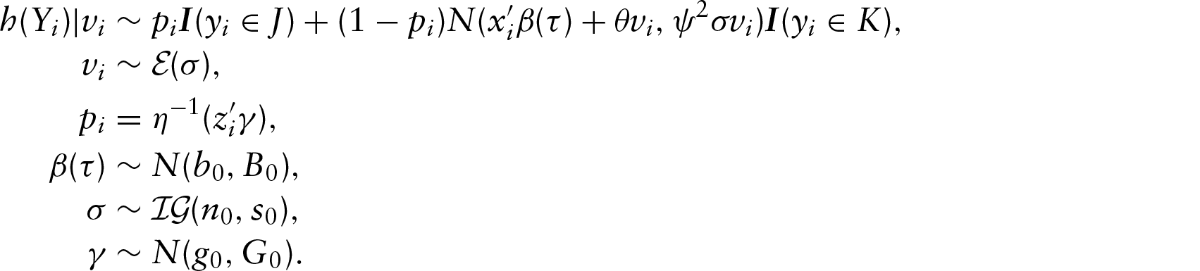
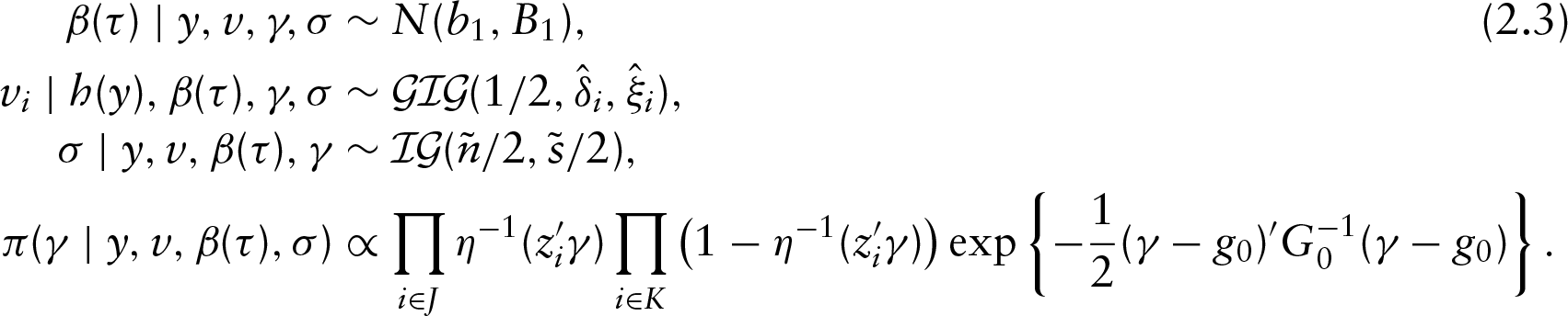
Furthermore, in all Bayesian models, an important part in the set-up is prior elicitation. Throughout the article, we decided to use only diffuse priors, as these have not presented any problems and the posterior distribution seems to be insensitive to minor changes. In this case, we consider, for example,
Moreover, all other full conditional distributions are relatively easy to generate posterior samples. The instructions to use our R code are available in the online supplementary material of this article.
Going back to the problem of studying expenditures in durable goods in a determined period, we have that a proportion of households might not have made any purchase for these kinds of items, having zero as the total of expenditures. This result was analysed using two different approaches in Tobin (1958) and Cragg (1971). Here we aim to combine these ideas, while making inference about the conditional quantiles of the continuous element of this type of problem. In the biometrics literature, Moulton and Halsey (1995) proposed an extension of Cragg's model, considering that an observed zero, or a lower detection limit, can be either from the point mass distribution or from the continuous distribution, being in the latter case a censored observation. Chai and Bailey (2008) considered a similar formulation, but changed the distribution of the continuous part and also the link function to model the probability
In this case, we should rewrite the density in (2.1) as

The latent variable
For the complete cases, define the sets

It is important to note that

In our quantile regression models, for the censored observations, we consider the idea proposed by Chib (1992) and adapted for quantile regression by Kozumi and Kobayashi (2011), which samples

If we define the variable

To complete the specification for this censoring variable, we have that for non zero observations
Plots for the probability of being censored for different
’s as a function of the probability
. (a)
, (b)
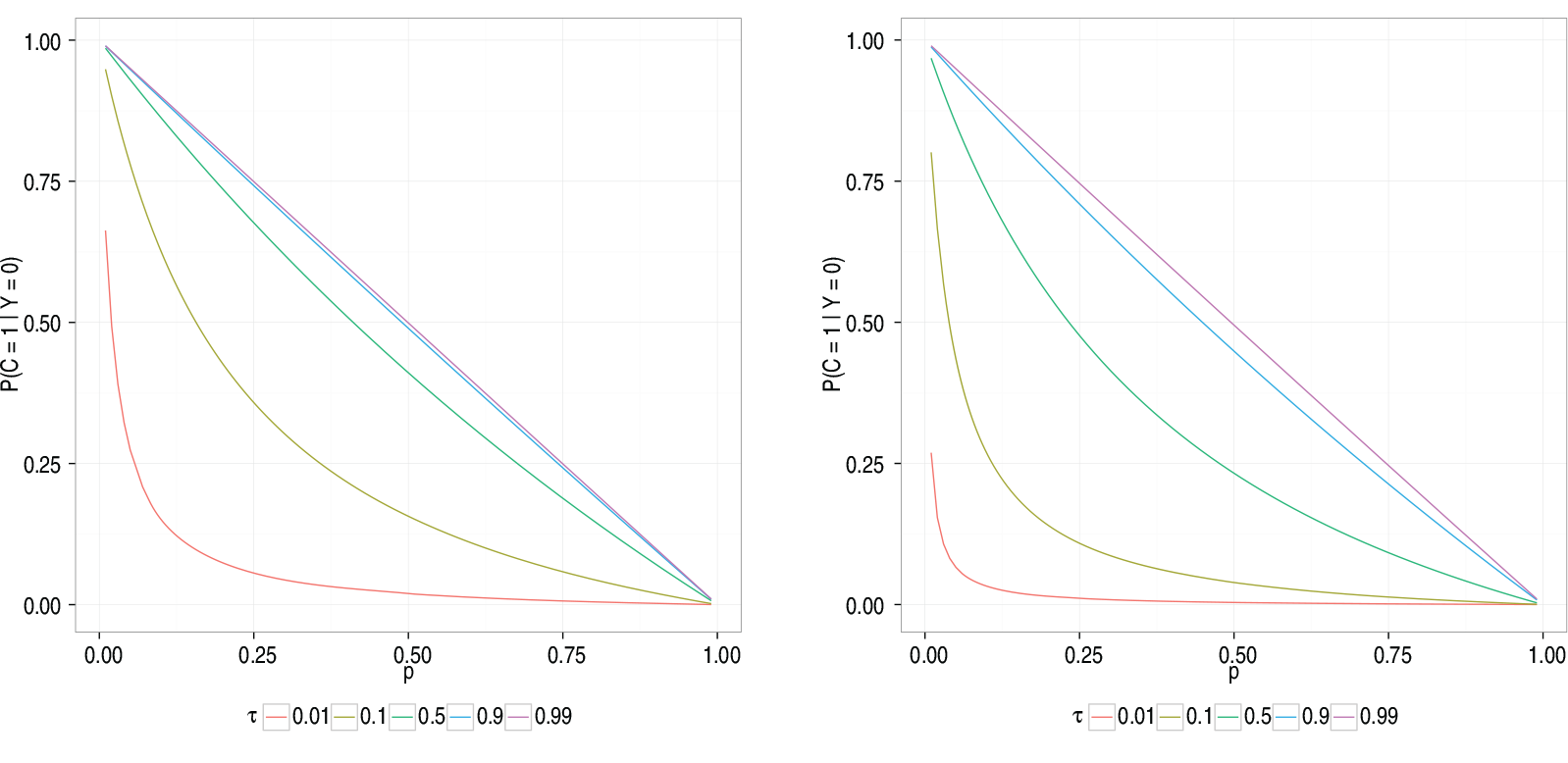
However, instead of evaluating

A posterior estimate of the probability of being censored for each observation can be calculated as

In this section, we are concerned in checking the performance of our model regarding its capability of making statements about the probability of being censored given that a certain observation has its response value equal to zero. In order to accomplish that, we replicate a study where we know which observations are censored and also which ones are not censored, between those with zero as their response value, and we compute this probability of interest for each group.
We consider a model with just two covariates and the following structure as

For each simulation, we calculate the probability of being censored for all observations with

Density estimate for the mean posterior probabilities of being censored for censored observations and also non-censored observations, based on 1 000 replicates for each scenario using a Gaussian smoothing kernel

Density estimate for the mean posterior probabilities of being censored for censored observations and also non-censored observations, based on 1 000 replicates for each scenario using a Gaussian smoothing kernel
In Figure 2, we plot the estimated density for the 1 000
Besides the interest in estimation of the probability of being censored, it is important to check whether the uncertainty about whether zero observations are censored or not undermine the estimation process of other parameters. There is just one note about the length of the MCMC chains in this simulation example, as we acknowledge that these sample sizes are small for the algorithm with a Metropolis–Hastings step, but we believe that this compromise was necessary due to time constraints in order to get the results in this simulation study.
Density estimate for parameters
,
and
,
based on 1 000 values for each parameter using a Gaussian smoothing
kernel
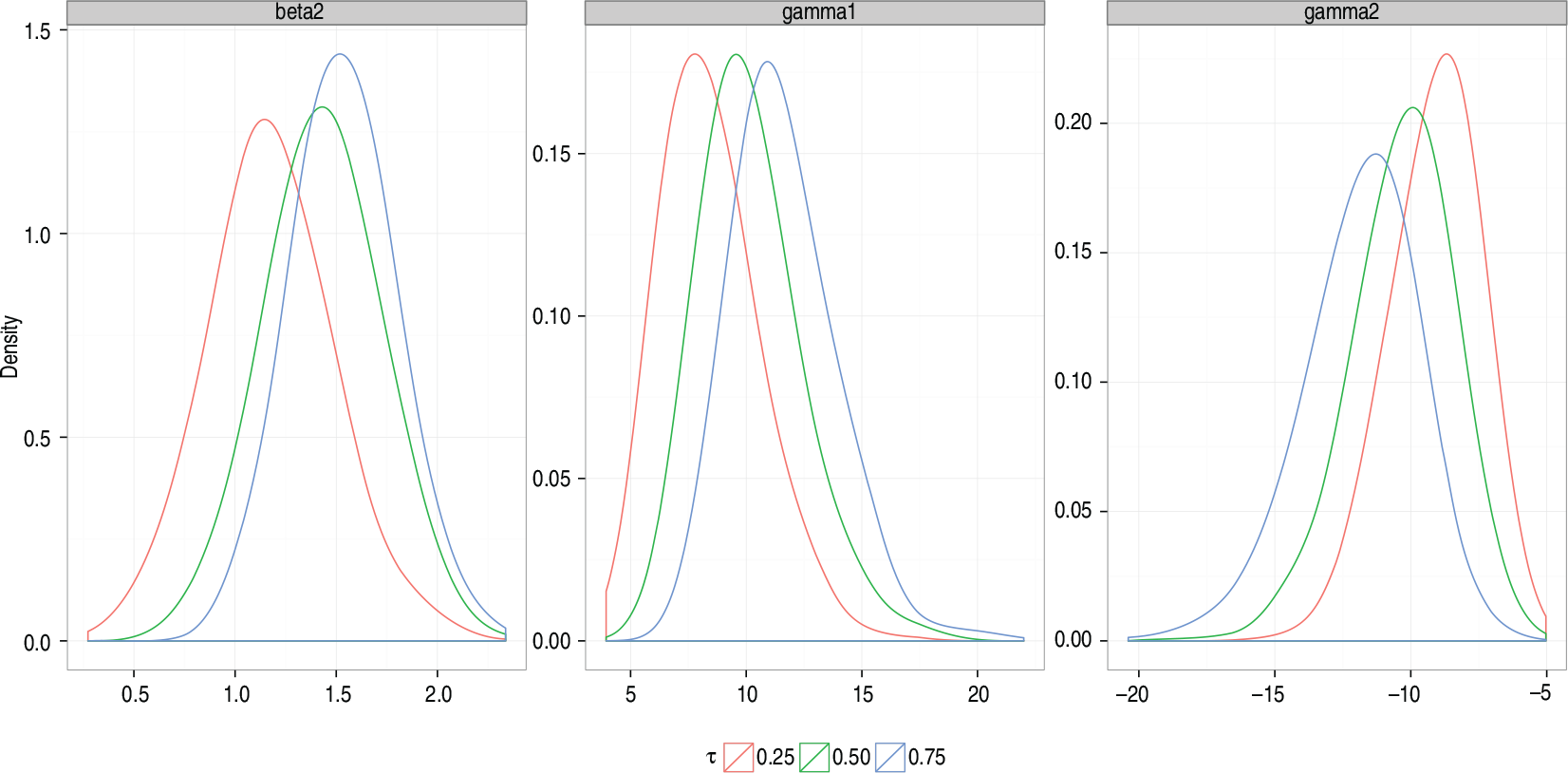
The density of the 1 000 posterior estimates of
Ultimately, we do not add another distribution for the error in this study, instead of the normal distribution, as we believe that such a change would not provide more information about the effectiveness of our model. Moreover, considering a larger sample would be helpful, as we expect that estimate errors would decrease with larger samples, but since the results were already satisfactory for this sample size, we decided not to continue any further. And adding more variables to each part of the model would definitely make the estimation process more difficult, but then we understand that this is a complication with which the algorithms could deal separately.
We exemplify our model with two applications. First, we consider the data from Mroz (1987), which was used for illustration purposes of the Tobit quantile regression model in Kozumi and Kobayashi (2011). And second, we present data about expenditures with durable goods in Brazil between 2008 and 2009, motivated by earlier considerations about this type of data by Tobin (1958) and Cragg (1971).
Labour supply data
Analysing empirical models about female labour supply, Mroz (1987) collected data about 753 married women, aged between 30 and 60 years old. The response variable of interest here is the number of hours worked for pay during the year of 1975, measured in 100h. In the sample, which was collected from the ‘Panel Study of Income Dynamics’, there are 325 women who did not work in that year, so their response variable is equal to zero. In Kozumi and Kobayashi (2011), they used this dataset to exhibit the Tobit quantile regression model, where these zero observations are assumed to be left censored. In our model, we combine the probability of being censored with the probability of being equal to zero to provide a more comprehensive study of these women who did not work that year. For covariates, we select non-wife income (

In Figure 4, we present the densities of the probabilities of being censored given that a certain observation is equal to zero for distinct
Density estimates of the probability of being censored for 325 women who did not work in Mroz (1987), for

Density estimates of the probability of being censored for 325 women who did not work in Mroz (1987), for
Posterior mean and 95% credible interval for
,

Besides that, we are able to compare the variation for each variable in the model according to the probability of being censored, which is a new factor that we add with our model for this type of analysis. For example, taking into account the variables income which is not due to the wife and years of experience, there are interesting results when we compare groups with different values for this probability for two values of
Density of the variable nwifeinc separated in two groups according to their relative censoring probability in comparison with the mean probability in a given quantile, for
. Solid lines are for the group above the mean probability of being censored, while dashed lines are for the group below
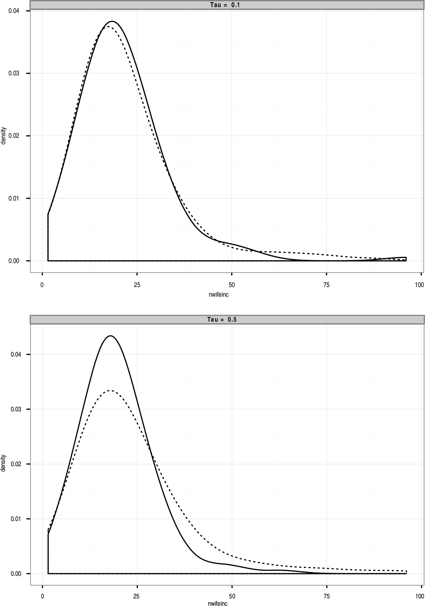
In Figure 6, we oppose the distribution of non-wife's income for women who have probability of being censored below and above the average for a specific quantile. For
Density of the variable educ separated in two groups according to their relative censoring probability in comparison with the mean probability in a given quantile, for
. Solid lines are for the group below the mean probability of being censored, while dashed lines are for the group above

Moreover, an analogous result is obtained with the variable years of experience and it is depicted in Figure 7, but now considering quantiles 0.5 and 0.9. Considering the probabilities of being censored for
Distribution of expenditures with durable goods, with a point mass at zero, in reais

Distribution of expenditures with durable goods, with a point mass at zero, in reais
We present here a second illustration of our model using data about household expenditures in Brazil, from the ‘Consumer Expenditure Survey’ that ocurred between 2008 and 2009, which is a national survey that interviewed more than 50 000 households around the country and it is available, in Portuguese, at
We include as covariates, gender (


We base our conclusions after running the MCMC obtaining 50 000 samples from the posterior distribution of the parameters of interest, from which we discarded the first 10 000 observations for burn-in purposes and later considered every 40th draw. As our estimator, we calculated the posterior mean for each parameter. Using these estimators, we see in Table 1, for the model of the probability
Mean posterior estimates and 90% credible intervals for
in model 5.1, for τ = 0.50
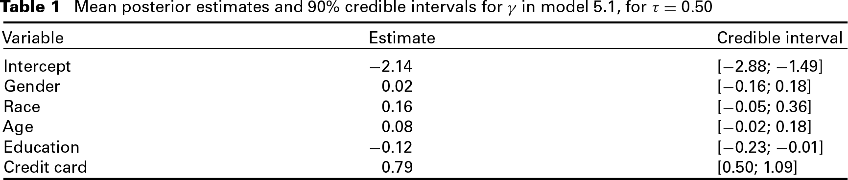
Mean posterior estimates and 90% credible intervals for

The posterior mean estimates for the continuous part are shown in Figure 9. Using quantile regression models, we are able to check if some variables have positive or negative effects in just some parts of the conditional distribution of the response variable. In this example, we find that difference between expenditures of men and women is different from zero only in the upper tail, or for
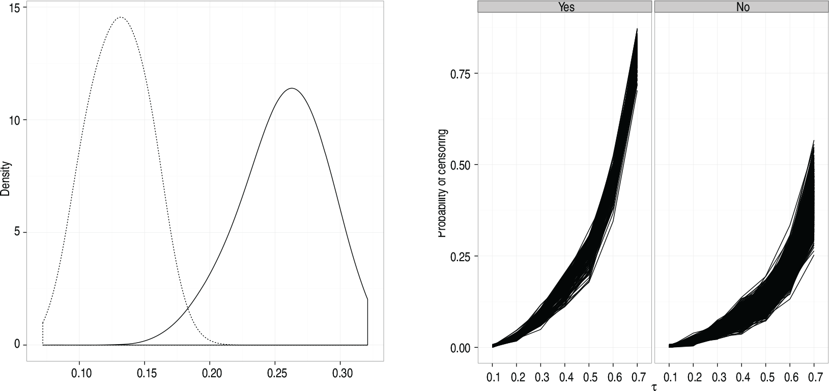
Analogous to the previous application, we can also compare the probability of being censored for different predictor variables. For
We do not show the probabilities for
Comparisons for the probabilities of being censored given the indicator variable credit card: (a) density estimates for
, yes = solid line, no = dashed line and (b) profiles of the probabilities for
In this article, we extended the Bayesian Tobit quantile regression model to include the probability of a response variable equal to zero being censored, instead of considering them censored observations from the beginning, using the asymmetric Laplace distribution in the likelihood to analyse the conditional quantiles of the continuous part of the model. We used a two-part model to study the probability of
Although this extension is based on the results obtained initially by Santos and Bolfarine (2015), we added an important feature in the modelling framework, which is the analysis of zero observations where the probability of being censored is taken into account for all zero observations. In the cited paper, the authors are only interested in measuring the difference between zero and non zero observations, while also studying the conditional quantiles for all observations in the continuous part of the model. Here, we showed how one can use the evidence in these two parts of the model to weight if a zero observation should be deemed censored given a fixed quantile or part of a point mass distribution at zero.
We showed how the probability of being censored, in our model, is dependent on the quantile of interest, providing more information about whether one observation should be considered indeed censored or not, for instance, comparing the profiles of probabilities from different observations and checking their variation for smaller or greater
We demonstrated our method in a simulated dataset, where we can control which observations are censored and which are non-censored, and we obtained contrasting estimates of the probabilities of being censored for these two types of observations when
In quantile regression models, it is always important to discuss the possibility of crossing quantiles, that is, if the expected ordering of
It is important to mention that our model could also be used in the survival analysis framework, when there is an assumption of a cure fraction in the study. Minor modifications would be necessary just to change the left censoring at zero for right censoring in this case. For future research, we are currently developing variable selection methods that try to share the information across both parts of the model and also when the variable selection method is quantile dependent.
Footnotes
Acknowledgments
This research was supported by the Fundação de Amparo à Pesquisa do Estado de São Paulo (FAPESP) under Grants 2012/20267-9 and 2013/04419-6.