An introduction to semiparametric function-on-scalar regression

Abstract

Abstract:

Function-on-scalar regression models feature a function over some domain as the response while the regressors are scalars. Collections of time series as well as 2D or 3D images can be considered as functional responses. We provide a hands-on introduction for a flexible semiparametric approach for function-on-scalar regression, using spatially referenced time series of ground velocity measurements from large-scale simulated earthquake data as a running example. We discuss important practical considerations and challenges in the modelling process and outline best practices. The outline of our approach is complemented by comprehensive R code, freely available in the online appendix. This text is aimed at analysts with a working knowledge of generalized regression models and penalized splines.

Keywords

Functional regression Functional response generalized additive model semiparametric regression penalized splines geophysics

1 Introduction

Regression models for functional responses try to model structures like time-dependent processes or 2D or 3D images (Ramsay and Silverman, 2005). Functional data are thereby defined as data that vary over a specific domain 𝒯, for example, time. Observations typically consist of measurements at individual points over that domain.

One valid alternative to functional response regression for data structured like this is longitudinal data analysis, modelling the separate measurements along each function using scalar regression while explicitly specifying their temporal correlation structure, for example, by including (random) time effects or by assuming autocorrelated residuals over time. However, eliciting an appropriate correlation structure is usually non-trivial. Using functional regression, correlation structures over the functional domain can be modelled flexibly and implicitly.

A functional approach should be the method of choice if the shape of a response over its functional domain is of main interest. Functional regression models enable researchers to quantify how various parameters influence the expected level and shape of the functional responses.

If the response is of a functional nature and all predictor variables are constant over the functional responses’ domain, the corresponding model is a function-on-scalar regression model. This work gives an introduction to this model class aimed at researchers looking for a pragmatic overview on how to apply this method without having to dive deeper into the technical part of it. As such, our focus is on explaining general concepts rather than providing detailed mathematical explanations of the method. Furthermore, we list important practical considerations and give advice on which methods are needed in which situation. Throughout the text, we show how to apply the methods using real-world data.

Various approaches to model function-on-scalar data exist. Our main focus lies on the flexible framework of Greven and Scheipl (2017a) which covers models of the form

\begin{matrix} Y_{i} (t) | X_{i} & \sim F (μ_{it}, ν) \\ g (μ_{it}) & = β_{0} (t) + \sum_{r = 1}^{R} f_{r} (X_{ri}, t) . \end{matrix}

(1.1)

For all observational units

i = 1, \dots, n

, the functional response, evaluated at specific points

t

of the functional domain, is assumed to come from some given distribution

F

with conditional expectation

μ_{it} = 𝔼 (Y_{i} (t) | X_{i})

and dispersion and shape parameters

ν

. The expectation is connected to an additive predictor with a functional intercept

β_{0} (t)

and

R

potentially nonlinear covariate effects

f_{r} (\cdot)

by a pre-specified link function

g (\cdot)

. The covariate effects

f_{r} (\cdot)

each depend on a subset

X_{r}

of the covariate set

X

and can potentially vary over the functional domain 𝒯. More specifically, we refer to 𝒯 as the time domain, as this is the functional domain in our running example. All methods, however, are also applicable for other functional domains.

Well-written introductions to the basic concepts and philosophy of functional data analysis are given in Ramsay and Silverman (2005) and Ramsay et al. (2009). Reviews of current research can be found in Morris (2015) and Wang et al.(2015). Readers interested in an in-depth review of available implementations for function-on-function and scalar-on-function regression models are pointed to Greven and Scheipl (2017a). An alternative approach that is closely related to the approach used here was developed by Reiss et al. (2010).

We perform our analyses in R (R Core Team, 2016, v. 3.3.2) using the function pffr from the package refund (Goldsmith et al., 2016), which is based on the gam function for scalar additive regression from the mgcv package (Wood, 2006, v. 1.8-15). The refund package is a flexible and fully documented package for functional data analysis. This article is accompanied by the open source R package FoSIntro (Bauer, 2017), available on GitHub, which comprises several convenience functions for the work with function-on-scalar models based on pffr. The GitHub repository also contains code showing how to apply all methods shown in this article.

The article is structured as follows: Section 2 introduces the running example for this work. Important statistical aspects of semiparametric regression are sketched in Section 3. Section 4 discusses concepts and challenges of function-on-scalar regression. We finish with a discussion and outlook in Section 5.

If the main interest lies in predicting or analysing specific characteristics of the functional response, alternative approaches are often more adequate. In particular, the function-on-scalar regression approach presented here is not well suited for predicting peak ground velocities as the penalized estimation of smooth structures tends to systematically underestimate the maxima.

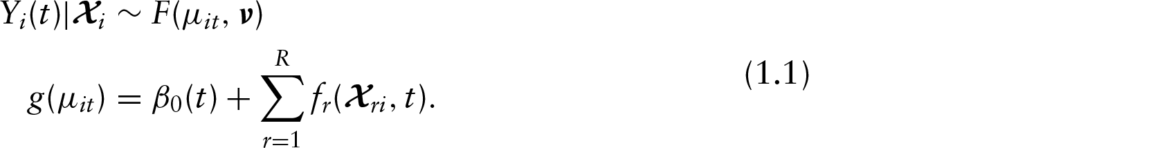
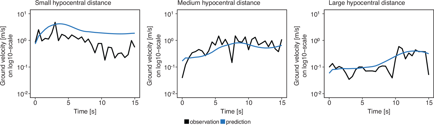
2 Application to seismic ground motion data

Bauer (2016) used function-on-scalar regression to quantify how frictional failure across an earthquake fault affects ground velocities at different distances from the earthquake's hypocentre over time. Figure 1’s left panel shows three typical observations of the functional response ground velocity over the functional domain time. All covariates in the study were constant over time.

Figure 1:

Left: Typical observations of absolute ground velocity over time. Peak ground velocity is delayed and decreases as the hypocentral distance increases. Middle: Overall functional mean of the ground velocities based on model (3.1) which only contains the intercept. Right: Estimated mean ground velocities by categorized hypocentral distance, based on model (3.2)

The aim of statistical modelling is to gain a better understanding of the associations between initial seismic conditions like fault stress and fault strength prior to earthquakes as well as local topography and geology with the temporal and spatial distribution of ground movement caused by an earthquake. The data is derived from large-scale in silico earthquake scenario simulations with the open source software SeisSol (Breuer et al., 2014; Pelties et al., 2014 www.seissol.org), based on a real seismic event that took place in Northridge (California) in 1994. Multiple simulations with varying initial conditions are analysed.

Shaking velocity and ground movement was recorded in high temporal resolution at a dense network of virtual seismometers distributed across Southern California. In the notation of (1.1), each response function $Y_{i} (t)$ represents the first 15s of the absolute ground velocity measurements from one of 75 such simulations for a given virtual seismometer $i$ in a resolution of 2Hz. A subset of 260 seismometers was used for the analysis. Leading zeros were discarded up to the first relevant ground movement ( $Y_{i} (t) \geq 0.01$ ) in order to remove irrelevant phase variation as described on p. 21. In keeping with the introductory level of this text, we only look at a submodel of Bauer (2016) and omit most seismological details.

The analysis is focused on the effects of five physical parameters on ground velocity: three frictional resistance variables, the direction of the regional tectonic background stress and the soil material of the simulated area: either rock or sediment. These parameters were pre-set in each seismic simulation. As seen in Figure 1, distance from the fault has an important effect on both the shape and the level as well.

3 Basic concepts of semiparametric modelling

The regression framework introduced by Greven and Scheipl (2017a) is based on additive or semiparametric regression models. Such models are one approach for estimating nonlinear effects of variables. In the following, we will introduce the basic modelling concepts of semiparametric functional regression by practically motivating differently complex models, each followed by a brief summary of the most important methodological basics.

3.1 Semiparametric models with one-dimensional smooth effects

In the simplest setting, we estimate the overall functional mean of ground velocities using a model only containing a functional intercept and no covariates:

g (𝔼 (Y_{i} (t))) = β_{0} (t) .

(3.1)

As the response in our application is strictly positive, we assume a Gamma distribution with a log link function

g (\cdot)

in all examples throughout this article. Figure 1’s middle panel shows this overall estimated functional mean for Equation (3.1). It can be seen that the overall mean is increasing over the first few seconds until it reaches a constant level.

As a next step, we want to assess a possible association of ground velocities with hypocentral distance, that is, we also want to quantify just how different curves at different hypocentral distances are on average. This can be done by extending Equation (3.1) with a dummy-coded categorical covariate $x$ for grouped hypocentral distance

g (𝔼 (Y_{i} (t) | x_{i})) = β_{0} (t) + β_{1} (t) I_{medium} (x_{i}) + β_{2} (t) I_{large} (x_{i}),

(3.2)

where

I_{medium} (x_{i})

is 1 if the hypocentral distance

x_{i}

of the station where observation

Y_{i} (t)

was recorded is intermediate, and 0 otherwise. Interpretation of categorical effects is equivalent to scalar regression, meaning that each effect

β_{1} (t)

and

β_{2} (t)

quantifies a deviation from the reference category ‘small distance’. As can be seen in Figure 1’s right panel, the estimated effects in Equation (3.2) show relevant differences in their level and shape.

3.2 Estimating one-dimensional smooth effects

Estimation of the functional intercept and the time-varying distance category effects is performed using a spline-based approach, where the effect is represented as the sum of scaled spline basis functions. Readers not familiar with this and other basic concepts regarding penalized estimation for generalized additive models are pointed to Fahrmeir et al. (2013) or Wood (2006). In a nutshell, penalization is a useful tool in estimating smooth effects as it allows estimation of nonlinear effects simply by defining the maximally possible wiggliness of each effect's shape, which is limited by the number of spline basis functions being used for that effect. Overfitting is then prevented by using an estimation criterion that punishes complexity of the effect estimates (i.e., wigglier shapes) while simultaneously rewarding goodness of fit. Parameters that control the relative weights in this trade-off between a good fit of the training data on one hand and a parsimonious model with simple effect shapes that is more likely to generalize well for previously unseen test data on the other hand are estimated from the data automatically.

Many different spline bases are available for one-dimensional smooth effects, cf. the documentation for mgcv. P-splines (Eilers and Marx, 1996) with second order difference penalties as well as thin plate regression splines (TPRS, see Wood (2003), based on Duchon (1977)) correspond to a weak prior assumption of linear effects. By default, pffr uses cubic P-splines with first order differences over the functional responses’ domain. This yields smooth effects and corresponds to a weak prior assumption of effects being constant over 𝒯. TPRS bases often perform slightly better than P-splines (Wood, 2003), but also suffer from numerical problems in some situations and are much more computationally expensive to set up.

Some more specialized spline bases are very useful in particular situations and easily available in the software we use here, for example, cyclic splines for periodic effects where boundary values must be equal or soap film smooths for fits with constraints along complex domain boundaries like seashores. Morris (2017) compares a Bayesian wavelet-based approach well suited for spiky data on regular grids to the method described here.

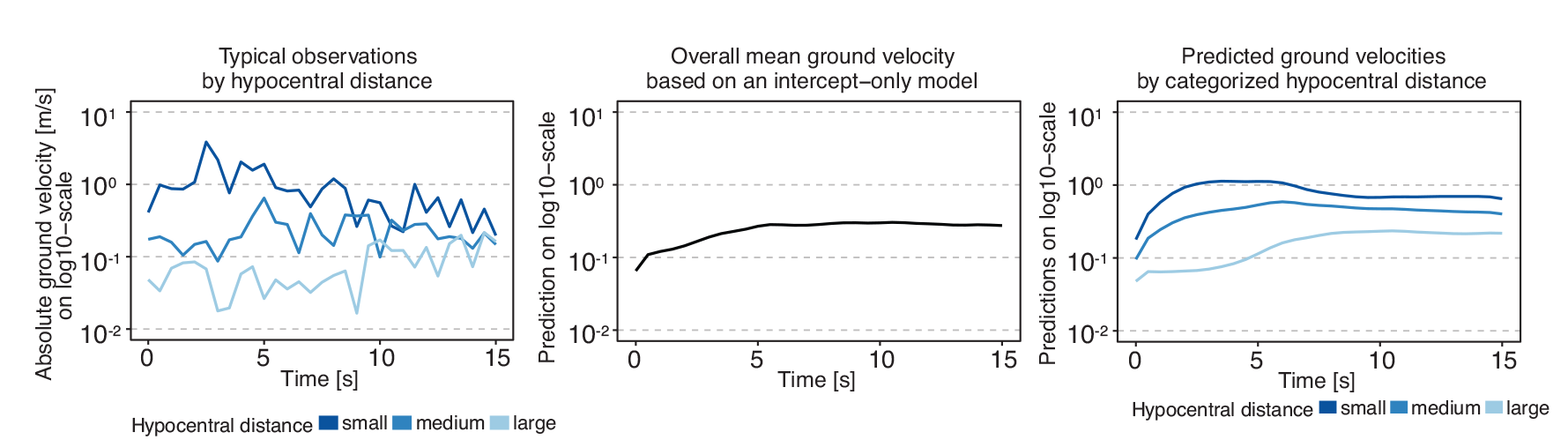
Using the spline-based approach, both the estimation of time-varying effects and of effects that vary nonlinearly over the variable domain itself is possible. An example for the latter is given in Figure 2’s left panel, which shows the estimated effect of the variable slip weakening, that is, the distance over which initial friction diminishes to its minimum. Higher values in this parameter correspond to bigger overall friction and thus to ground velocity curves that have a lower level overall. Note that this type of time-constant effect does not affect the shape of the functional responses, only their overall level.

Putting all currently described effect shapes together, we are now capable of specifying models of the form

g (𝔼 (Y_{i} (t) | X_{i})) = β_{0} (t) + \sum_{j = 1}^{J} β_{j} (t) x_{ji} + \sum_{k = 1}^{K} f_{k} (x_{ki}),

(3.3)

which include

J

time-varying linear effects

β_{j} (t)

as well as

K

smooth effects

f_{k} (\cdot)

which are time-constant, but vary over the respective variables

x_{k}

3.3 Semiparametric models with multidimensional smooth effects

As a final step, we now include multidimensional smooth effects into the model. Such effects can vary nonlinearly both over the domain of the functional response and the domain of the covariate (or multiple covariate domains in the case of interaction effects). As an example, the three rightmost panels of Figure 2 visualize the estimated nonlinear time-varying effect of the hypocentral distance. To facilitate interpretation of the effect, it is shown using both a heatmap (panel 3) as well as a 3D surface (panel 4). In addition, a comparison of the predictions for specific values is a valuable tool as well (panel 2). One can see (a) that smaller hypocentral distances correspond to higher ground velocities (note the large negative slope of the estimated surface along the distance axis), (b) that the initial peak of ground velocity sets in later the farther away from the earthquake centre the virtual seismometers are located (note that the peak for a given distance is located higher up the time axis as distance increases), (c) that the peak becomes somewhat less pronounced for larger distances and (d) that the effect is almost linear over hypocentral distance.

Figure 2:

Panel 1: Estimated time-constant effect of slip weakening f_slip(x_slip), which implies a (nonlinear) shift in the average level of $Y_{i} (t)$ as x_slip changes. 2: Predictions for specific values of hypocentral distance with remaining covariates set to realistic values. 3, 4: Effect of hypocentral distance visualized using a heatmap and a 3D surface. Note that values in panels 1, 3 and 4 are on the scale of the additive predictor (i.e., log_e([m/s])), while panel 2 is on log₁₀-scale

3.4 Estimating multidimensional smooth effects

Incorporation of multidimensional smooths into Equation (3.3) is easily done by generalizing it to

g (𝔼 (Y_{i} (t) | X_{i})) = β_{0} (t) + \sum_{r = 1}^{R} f_{r} (X_{ri}, t) .

(3.4)

In addition to the functional intercept we now have

R

covariate effects

f_{r} (X_{ri}, t)

which potentially vary over both covariate domains and the functional domain 𝒯. We write

X_{ri}

instead of

x_{ri}

to emphasize that each smooth potentially depends on multiple covariates, thereby covering linear interactions terms and multidimensional smooths. Note that

f_{r} (\cdot)

can obviously also be a time-constant, linear effect.

We briefly sketch two possibilities for setting up a multidimensional spline basis for representing effects $f_{r} (X_{ri}, t)$ . Tensor product spline bases are created by setting up an adequate marginal one-dimensional basis for each dimension of the effect (e.g., hypocentral distance and the time domain) and then taking the Kronecker product of the marginal bases (i.e., multiplying each basis function of each marginal dimension with all basis functions of all other marginal dimensions). This results in a multivariate spline basis defined on the joint domain of all involved covariates (and time). A major advantage of this method is its large flexibility as the appropriate marginal bases and penalties can be chosen freely to suit the problem. Since penalization of such tensor product spline terms is done separately for each dimension, this also allows for different roughnesses of the various marginal dimensions (e.g., an effect $f (x_{r}, t)$ that is very smooth over some covariate $x_{r}$ but still wiggly over time $t$ ). A disadvantage of tensor product splines is that tensor basis functions are defined on a regular grid over the joint domain and some basis functions may lie in regions where there are not many or no data points at all, leading to computational inefficiencies and badly conditioned model fits. An alternative to tensor product spline bases are multidimensional TPRS, a direct generalization of the one-dimensional TPRS basis. The most important difference is that TPRS basis functions imply identical roughness in all directions. In practice, this only makes sense if marginal variables are on comparable scales, for example, in a 2D spatial effect with longitude and latitude as the marginal covariates.

3.5 Some practical considerations

Since the number of basis functions limits the maximal complexity of the shape of any effect $f_{r} (X_{ri}, t)$ , it needs to be sufficiently large. Which number to choose initially depends greatly on the data situation and it is very difficult to provide general advice. For most applications, 20-30 basis functions for a one-dimensional effect will typically be sufficient, but this is feasible only if enough observations are available for estimation. In situations with fewer data points or simple effect shapes, however, it can also be appropriate to use only 5 or 10 basis functions initially. After estimating the model, the effective degrees of freedom (edf; see Wood, 2006, Ch. 4.4) of each term give an indication of whether the amount of flexibility was sufficient or not. If the edf are near their maximum, the model should be re-estimated using a larger number of basis functions. In this case, a larger basis that is expressive enough for the effect's true complexity can improve the estimate. An automated approach for checking adequacy of the chosen basis dimension was introduced by Pya and Wood (2016) and is implemented in the gam.check function of R package mgcv.

In some situations, the placement of the basis functions over the effect's domain can be of great importance. If no further information is available an equidistant placement is a valid approach. In contrast, a user-specified placement can make sense if the data are spread very unequally across the domain and the researcher supposes that the effect will vary more strongly in regions where more data points lie or when a few data points lie far beyond the main data cloud. In such cases, it can be more efficient to place more knots in regions with more data, especially in situations with small to moderate sample size.

4 Inference and model checking

This section focuses on setting up and evaluating a function-on-scalar model. As motivated in the last section, the general model of Greven and Scheipl (2017a) can be written as

g (𝔼 (Y_{i} (t) | X_{i}, E_{i} (t))) = β_{0} (t) + \sum_{r = 1}^{R} f_{r} (X_{ri}, t) + E_{i} (t),

(4.1)

where the conditional expectation of the response

Y_{i} (t)

is modelled by

R

potentially nonlinear effects (as defined on p. 10) and a functional intercept

β_{0} (t)

. The newly introduced term

E_{i} (t)

specifies functional error terms. Those smooth errors are estimated as curve-specific functional random intercepts and can be used to incorporate possible autocorrelation and variance heterogeneity along the functional domain (Scheipl et al., 2015) as motivated in the next paragraph. The additive predictor is mapped to the domain of the functional responses by a given link function

g (\cdot)

, which for the Gamma-model in our application example is simply the natural logarithm. Note that the interpretation of effects in models including (functional) random effects like

E_{i} (t)

is generally conditional, not marginal, similar to conditional GLMMs (Diggle et al., 2002): the estimates quantify the expected change in individual conditionally expected values, not in population averages. This distinction is meaningless if the link function

g (\cdot)

is the identity, that is, for Gaussian models.

In many practical applications, the assumption of independence along $t$ conditional on the additive predictor for each functional response is not borne out and observed residuals are correlated (and frequently heteroscedastic) along $t$ . This can easily be diagnosed by computing the empirical covariance and correlation of the residuals (see panel 4 of Figure 4, p. 24). If residual intra-curve correlations are non-negligible, confidence intervals (CIs) and tests will be overly optimistic. If computationally feasible, models should then include functional smooth residuals $E_{i} (t)$ to account for such autocorrelation and variance heterogeneity.

Generally speaking, all response distributions from scalar regression are also available for use in models with a functional response. Whether effects are constant or varying over the functional domain should be investigated for all variables (metric and categorical). How appropriate effect types can be determined as part of the modelling process is outlined in Section 4.4.

4.1 Uncertainty quantification

CIs for smooth effects can either be constructed globally (or simultaneously), pointwise or intervalwise, the interpretation being that the CI overlaps the true effect globally, at a specific point or in a specific interval with a given probability, respectively. This is an area of active research; see, for example, Krivobokova et al. (2010) or Marra and Wood (2012). As a generally applicable method, bootstrapping can be used to construct all different types of CIs. However, it can be computationally expensive—often prohibitively so for high-dimensional data or complex models.

Several bootstrap strategies exist that can be used in this context. The most established approach in the context of regression modelling is the conditional or parametric bootstrap (Efron and Tibshirani, 1994), which consists of the following steps for constructing a pointwise CI for the linear coefficient $β_{1}$ based on a sample of size $n$ , but is also easily generalizable to compute intervalwise or global intervals:

Create $B$ bootstrap samples from the data. In each of the $B$ samples a new response value $y_{i}^{b}$ is generated for each observation $i$ by drawing a random value from the conditional response distribution specified by the regression model. In the Gaussian case, new response values $y_{i}^{b}$ can be drawn from the distribution

Y_{i} | X_{i} \sim N ({\hat{y}}_{i}, {\hat{σ}}_{ε}^{2}),

where

{\hat{y}}_{i}

is the model-based prediction for observation

i

and

{\hat{σ}}_{ε}^{2}

is the estimated error variance.

Calculate the model on each of the $B$ samples and save $β_{1}$ as $β_{1}^{b}$ , $b = 1, \dots, B$ .

Define the CI using empirical quantiles, for example, the 2.5% and 97.5% quantiles to obtain a 95% CI.

Note that parametric bootstrapping heavily relies on the underlying model being specified correctly. In case of violation of the model assumptions, this approach can lead to overly optimistic intervals and instead nonparametric bootstrapping should be used, where resampling is based on the raw data (Efron, 1979). Because of the exemplaric character of our running example we use nonparametric bootstrapping to estimate CIs.

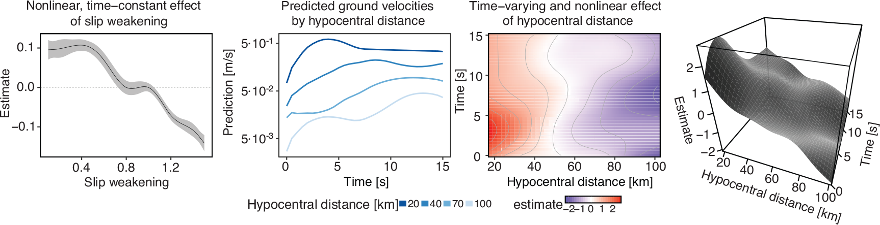
As an alternative to bootstrapping, the empirical Bayesian CIs developed by Marra and Wood (2012), which are an extension of Nychka's (1988) CIs, are computationally efficient and implemented in mgcv. However, Marra and Wood show that these intervals do not perfectly fulfil the property of pointwise CIs. Figure 3 shows a comparison of the CIs of Marra and Wood and real pointwise, bootstrap-based CIs, with the latter being ever so slightly wider throughout in this case. Considering, however, that differences between these two are usually small as long as the model is not severely misspecified, the Marra and Wood CIs are a useful tool to compute uncertainty of smooth estimates efficiently.

Figure 3:

Left: Comparison of the Marra and Wood (2012) CIs and pointwise, nonparametric bootstrap-based CIs (95%) using 1000 Bootstrap samples for the smooth effect of sediment velocity. Right: Pointwise, nonparametric bootstrap-based CIs (95%) and point estimate for the time-varying smooth effect of hypocentral distance using 1000 Bootstrap samples

In contrast to one-dimensional effects, visualization of uncertainty for multidimensional smooth effects is more complex as a 3D surface plot cannot be used to show both the point estimate and CIs. Instead, the best approach is to use separate heatmaps for the point estimate, the lower CI boundary and the upper CI boundary using identical colour legends, as shown in Figure 3. Looking at the estimates, it can be seen that the uncertainty about the effect of hypocentral distance is rather small.

Regarding predictions, both pointwise CIs for the predicted mean values and pointwise prediction intervals can be obtained based on Wood (2006, Ch. 1.3.6). For intervalwise or global versions of both interval types again bootstrap-based methods have to be used, but our practical experience suggests that the differences to pointwise CIs are usually negligible for practical purposes.

4.2 Hypothesis testing

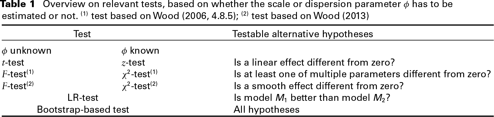
Most of the relevant hypotheses in function-on-scalar regression can be tested using the five test approaches listed in Table 1. All tests apart from the bootstrap are Wald-like tests which are based on the approximate normal distribution of the estimated regression coefficients. For details, see Wood (2013) and Marra and Wood (2012). The appropriate test distribution mostly depends on the question whether the scale or dispersion parameter $ϕ$ has to be estimated or not (Wood, 2006). For a normal response $ϕ = σ^{2}$ is generally unknown, whereas the use of Poisson or Binomial responses implies a known value of $ϕ = 1$ .

Table 1:

Overview on relevant tests, based on whether the scale or dispersion parameter ϕ has to be estimated or not. ⁽¹⁾ test based on Wood (2006, 4.8.5); ⁽²⁾ test based on Wood (2013)

Test		Testable alternative hypotheses
$ϕ$ unknown	$ϕ$ known
t-test	z-test	Is a linear effect different from zero?
F-test $^{(1)}$	$χ^{2}$ -test $^{(1)}$	Is at least one of multiple parameters different from zero?
F-test $^{(2)}$	$χ^{2}$ -test $^{(2)}$	Is a smooth effect different from zero?
LR-test		Is model $M_{1}$ better than model $M_{2}$ ?
Bootstrap-based test		All hypotheses

Hypotheses for scalar coefficients of the form $β_{j} = 0$ can be tested using a t-test. For testing multiple $β$ ’s being zero at the same time an F-test can be used (Wood, 2006, Ch. 4.8.5). A different F-test based on the test statistic introduced in Wood (2013) is available to test whether a nonlinear effect is significantly different from zero. Note that this is a test only for the global hypothesis. For a pointwise or intervalwise evaluation, a bootstrap-based approach has to be used. As in the previous section, a bootstrap is hereby used to create an appropriate CI and as a second step the null hypothesis is rejected if zero is not (or at no point for an intervalwise test) inside of the CI. Finally, specific hypotheses can also be tested by comparing models using likelihood ratio (LR)-tests (Wood, 2006, Ch. 4.10.1). Be aware that an LR-test can only be used for model comparison if the two models are nested. Some more information on model comparison is given in Section 4.4.

Note that all the tests given earlier are conditional on the estimated penalty parameters that control the effective degrees of freedom of each term. However, neglecting smoothing parameter uncertainty does not seem to have a large negative impact on the validity of p-values and the performance of CIs unless penalty parameters are poorly identified (Marra and Wood, 2012). An approach to account for smoothing parameter uncertainty in p-value calculation is outlined in Wood et al., (2016b) and implemented in mgcv as well (see Vc in ?gamObject).

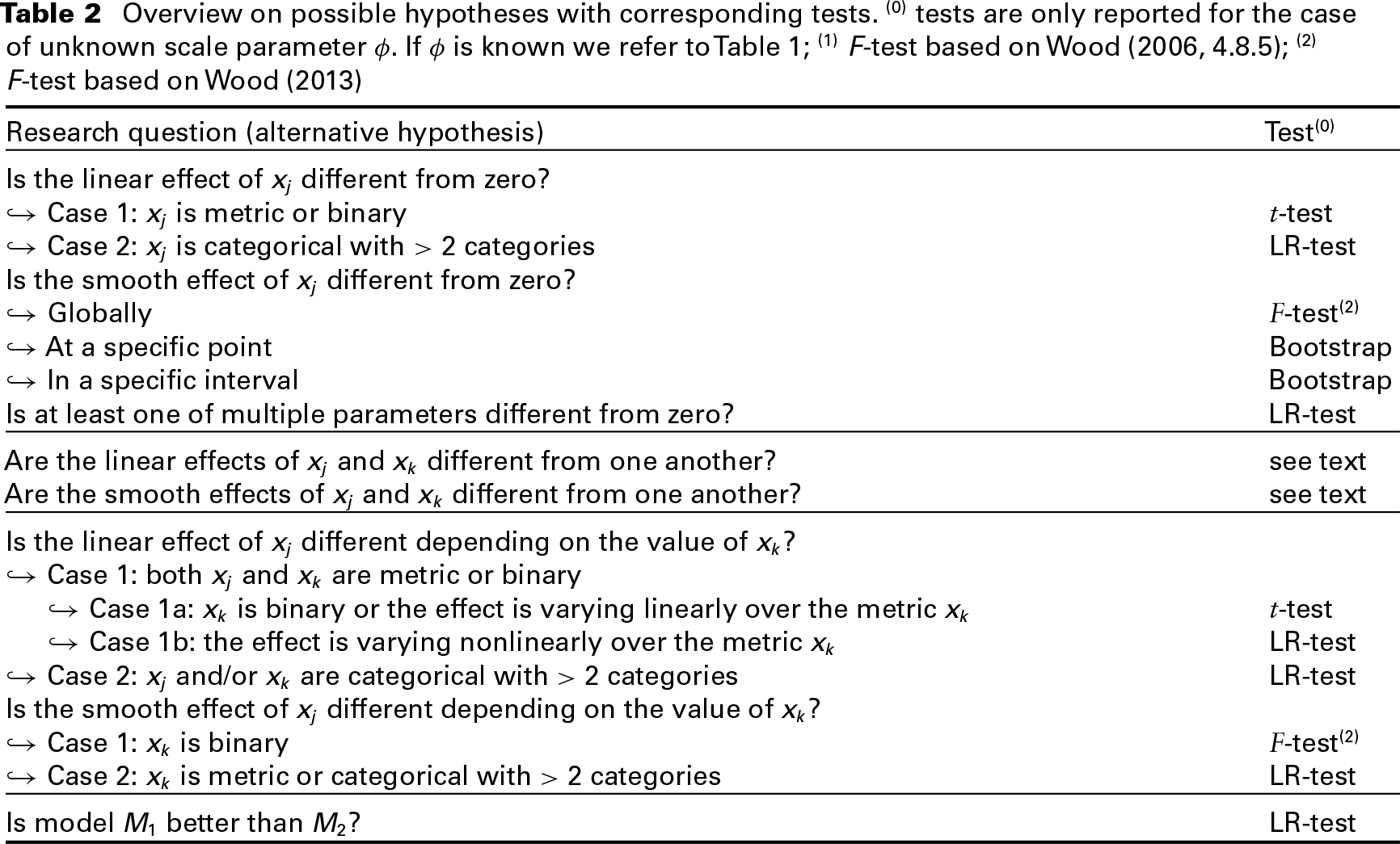
An overview on the most important hypotheses in function-on-scalar regression is given in Table 2, which lists possible research questions together with the appropriate tests. As a special note, testing whether two scalar effects (or two smooth effects) of $x_{k}$ and $x_{j}$ are different from one another only arises in situations where, for example, two treatments $x_{k}$ and $x_{j}$ (with time-varying effects) should be compared. Thus, this can be translated into another hypotheses by using one treatment as the reference category and then testing the hypothesis ‘Is the linear (or smooth) effect estimating the difference between treatments different from zero?’

Table 2:

Overview on possible hypotheses with corresponding tests. ⁽⁰⁾ tests are only reported for the case of unknown scale parameter ϕ. If ϕ is known we refer to Table 1; ⁽¹⁾ F-test based on Wood (2006, 4.8.5); ⁽²⁾ F-test based on Wood (2013)

Research question (alternative hypothesis)	Test $^{(0)}$
Is the linear effect of $x_{j}$ different from zero?
$↪$ Case 1: $x_{j}$ is metric or binary	t-test
$↪$ Case 2: $x_{j}$ is categorical with $> 2$ categories	LR-test
Is the smooth effect of $x_{j}$ different from zero?
$↪$ Globally	F-test $^{(2)}$
$↪$ At a specific point	Bootstrap
$↪$ In a specific interval	Bootstrap
Is at least one of multiple parameters different from zero?	LR-test
Are the linear effects of $x_{j}$ and $x_{k}$ different from one another?	see text
Are the smooth effects of $x_{j}$ and $x_{k}$ different from one another?	see text
Is the linear effect of $x_{j}$ different depending on the value of $x_{k}$ ?
$↪$ Case 1: both $x_{j}$ and $x_{k}$ are metric or binary
$↪$ Case 1a: $x_{k}$ is binary or the effect is varying linearly over the metric $x_{k}$	t-test
$↪$ Case 1b: the effect is varying nonlinearly over the metric $x_{k}$	LR-test
$↪$ Case 2: $x_{j}$ and/or $x_{k}$ are categorical with $> 2$ categories	LR-test
Is the smooth effect of $x_{j}$ different depending on the value of $x_{k}$ ?
$↪$ Case 1: $x_{k}$ is binary	F-test $^{(2)}$
$↪$ Case 2: $x_{k}$ is metric or categorical with $> 2$ categories	LR-test
Is model $M_{1}$ better than $M_{2}$ ?	LR-test

Apart from the penalized likelihood-based (or empirical Bayesian) framework introduced here, fully Bayesian inference like, for example, the framework of Morris (2017), see Section 4.6, often allows for easier handling of complex or non-standard inferential problems. When relying on the software implementation of the Greven and Scheipl (2017a) framework in the R package refund, Bayesian estimation of all exponential family models is available using the automatic translation of the model specification and model data into JAGS (Plummer, 2016) code using mgcv’s jagam function (Wood, 2016) for automated, tuning-free, fully Bayesian inference based on Markov Chain Monte Carlo sampling.

Working with generally high-dimensional functional data, researchers should be aware that, all else being equal, large sample sizes lead to smaller p-values in the case of $H_{0}$ not being true. In such cases, importance should not be attached primarily to p-values of point hypotheses of ‘no effect’. Instead, best practice in interpreting regression results is based on well-founded discussion of the relevance of the estimated effect strength and its associated uncertainty while considering whether the sample is appropriate for drawing general conclusions from it. Having quite high-dimensional data ourselves, we do not report specific test results for our running example.

4.3 Some specific challenges

We now list some further challenges that are specific to dealing with functional data. A first comparison of different modelling approaches regarding those problems is given and is complemented by the main discussion in Section 4.6.

If the functional responses have hierarchical, longitudinal or spatio-temporal structure, there may be non-negligible inter-curve correlation that the model has to account for. In the case of grouped data, that is, longitudinal or hierarchical data, functional random intercepts and slopes varying over the functional domain of the response can be incorporated into the model (Greven and Scheipl, 2017a). Spatio-temporal correlation with a pre-specified structure between functional responses can be included explicitly by including smooth effects over space or time. Scheipl et al. (2015, Online Appendix C) contains a worked example and code for spatially correlated curves.

Another common problem when dealing with time-varying functional data is misalignment or phase variation of functional observations. This means that certain salient features of the functional responses like peaks or plateaus do not occur at the exact same time points. Few functional data analysis frameworks are currently able to incorporate both phase and amplitude variation (cf. fdasrvf, Tucker, 2016) and we are not aware of any implementation of functional response regression able to do so. Ignoring misalignment typically results in blurred estimates. Therefore, an appropriate pre-processing of the data is necessary, for example, to align all peaks at the same time points. An overview on methods tackling phase variation in functional data analysis is given by Marron et al. (2015). In our application, ground velocity curves are heavily misaligned since the seismic shock waves take longer to reach seismometers further away from the hypocentre and the corresponding curves thus remain at (close to) zero for longer times. We pragmatically solve this problem by removing leading zeros before model estimation.

Functional data are frequently high-dimensional and estimation of complex models can be very expensive, both in terms of computation time and memory requirements. Pragmatically speaking, analysts facing such a problem should consider downsizing the data, for example, by reducing the resolution of functional measurements over the functional domain or by using only a subset of the data for estimation and the remainder for model validation. Highly efficient estimation algorithms are available for some approaches. For the class of spline-based models we focus on here, one can use the algorithm of Wood et al. (2016a), which is implemented in the function bam in R package mgcv (Wood, 2006), also accessible via pffr. The fully Bayesian wavelet-based approach of Morris (2017) and collaborators, implemented in the WFMM software (Herrick, 2015) has excellent scaling behaviour for time and memory both in terms of data set size and model complexity.

Finally, users should be aware that some methods for functional data are only applicable if the functional observations contain no missing measurements and were observed on a regular grid, that is, all functional observations are evaluated at the same points of the functional domain. A comparison of the applicability of various function-on-scalar regression frameworks is given in Section 4.6.

4.4 Model selection

Generally speaking, model selection in functional regression models underlies the same principles as in scalar regression (see, e.g., Marra and Wood, 2011; Fahrmeir et al., 2013, Ch. 3.4.3). Using model selection in function-on-scalar regression can be useful for various issues, for example, for deciding which response distribution and link function is optimally suited to the data or whether an effect should be incorporated linearly or as a smooth curve. Additionally, very high-dimensional data often reduces the effectiveness of penalization methods as the information in the observed data overwhelms the penalization prior (Gelman et al., 2014). In such situations it can be necessary to use model selection to optimize the number of basis functions for each smooth effect.

Leeb and Pötscher (2005) propose a test set based approach to prevent overfitting and preserve valid p-values when performing model selection. For smaller datasets, k-fold cross validation is a valid alternative (Hastie et al., 2009). Using one of those two approaches, the best model can, for example, be found by using the prediction error as the optimization measure. When model selection is based on training set performance, other criteria like AIC or LR tests should be used (Fahrmeir et al., 2013). Note that if using the semiparametric approach smoothing parameter uncertainty should be accounted for in AIC computation (see Wood et al., 2016b).

For our data, we use a test set based model selection approach with mean square prediction error (MSE) as the criterion for two purposes. First, penalization did not work very well in this setting, probably due to the massive amount of data available. Therefore, we use a pragmatic model selection procedure to select the number of basis functions for each smooth effect and to decide whether individual effects should be incorporated as a smooth effect or linearly. Second, we use model selection to choose between different response distributions and link functions.

4.5 Model evaluation

Model assumptions for functional response regression are mostly the same as in respective scalar models, that is, observations are independent conditional on the additive predictor. Model evaluation is mainly done by visualizing the residual structure.

Figure 4:

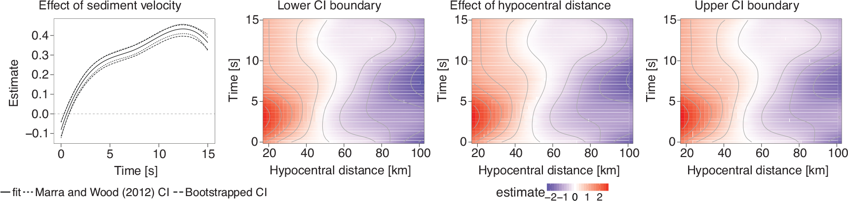
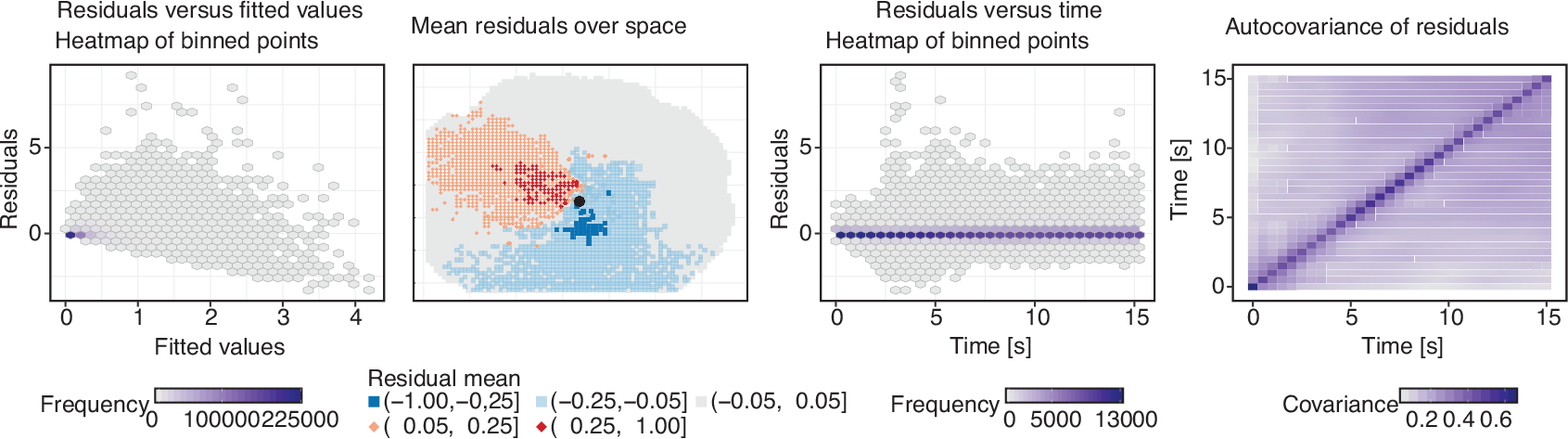
From left to right: Residuals versus fitted values, residuals versus space, residuals versus the functional domain, autocovariance of residuals over the functional domain. The black dot in the second plot marks the epicentre

A selection of useful residual plots is shown in Figure 4. The structure of the residuals plotted against the fitted values (panel 1) is acceptable. Most measurements are predicted approximately correct. The odd structure of negative residuals is based on the ground velocities being non-negative, which results in highly negative residuals not being possible. Plotting the mean residuals over space (panel 2) shows that a substantial spatial struture is remaining in the residuals. Nearly all regions where ground velocities were substantially underestimated are west of the earthquake centre, while seismometer readings in regions to the east and to the south of the epicentre were overestimated. Across time, however, we again observe an acceptable amount of residual structure—the hexbin plot (panel 3) does not show any systematic deviations from a constant trend at zero, with some extreme peak ground velocities observed at around five seconds. As functional data often are very high-dimensional standard scatterplots of the residuals, having the problem of overplotting should generally be avoided in favour of alternative plots like density plots or hexagonal binning (Carr et al., 2016), as was done in the left and middle plots of Figure 4. The empirical autocovariance of the residuals (panel 4) corresponds well enough to the model assumptions: it is fairly constant along the diagonal (i.e., the variance of the residuals is fairly homogeneous over functional domain $t$ ) and drops off quickly towards zero away from it (i.e., the autocorrelation of the residuals along $t$ is rather small and very short-range), slightly less so for $t > 10$ .

For an evaluation of the prediction power of the model, measures like MSE of the predictions can be calculated. We also recommend graphical evaluation of predictions for single functional observations as was done in Figure 5 to get an overview on model performance.

Figure 5:

Comparison of model predictions and raw observations for typical observations with different hypocentral distances

4.6 Alternative approaches and software implementations

As alternative approaches to semiparametric regression we only cover the most versatile frameworks for performing function-on-scalar regression. The capabilities of the respective software implementations are also outlined, a comprehensive comparison of available software implementations is given in Table 3 of Greven and Scheipl (2017b). Many specialized function-on-scalar regression methods have been proposed in the literature, oftentimes with corresponding small software implementations, which we do not cover here. See Morris (2015) for an in-depth review of this field.

The semiparametric approach of Greven and Scheipl (2017a) was already outlined extensively. The methodology is ready-to-use in the refund package in R (Goldsmith et al., 2016), the most versatile function therein being pffr.

One class of alternative approaches includes a pre-smoothing step prior to model estimation, meaning that each functional observation is smoothed and the resulting smooth curve is then treated as the functional observation (see, e.g., Ramsay and Silverman, 2005). The disadvantage is that the measurement error removed by the smoothing step is not taken into account in subsequent inference. On the plus side, this can allow for more efficient estimation as the smooth curve can then be represented compactly by the vector of spline coefficients yielding the smoothed curve. The R package fda is publicly available (Ramsay et al., 2014) and implements simple linear models for functional responses.

An overview of nonparametric methods and their applications is provided in Ferraty and Vieu (2006). Their regression approaches are usually based on kernel methods and are able to model highly nonlinear associations. However, the methods mostly cover only univariate models with a single covariate. Febrero-Bande et al. (2012) introduce the R package fda.usc which implements a subset of these methods and related extensions.

The componentwise gradient boosting framework of Brockhaus et al. (2016b) is spline based and extremely versatile. With boosting being a popular, very efficient yet very powerful estimation technique, it represents a neat alternative to the standard regression approach. The advantages are most noticeable when working with very high-dimensional data requiring an efficient estimation technique or when dealing with data situations with more parameters than observations, as such settings remain computationally feasible using a boosting approach. Also, the boosting approach automatically performs variable selection. However, uncertainty quantification for boosting is currently only possible using computationally expensive resampling techniques like bootstrapping (Hastie et al., 2009). The method is implemented in the R package FDboost (Brockhaus, 2016). Recently, this approach has also been extended to model the variance of functional responses conditional on covariates (Brockhaus et al., 2016a), using techniques developed in the literature on generalized additive models for location, scale and shape (GAMLSS; Mayr et al., 2012). More general details on boosting and GAMLSS can be found in the tutorials by Mayr and Hofner (2018) and Stasinopoulos et al. (2018), respectively, which are also part of this special issue.

As another alternative, fully Bayesian functional regression can be used. The most comprehensive framework we are aware of is the one of Morris (2017) and collaborators, who also provide a comprehensive comparison to the approach of Greven and Scheipl (2017a). Generally speaking, fully Bayesian approaches have the advantage that diverse between- and within-function correlation structures can be incorporated into the model in a very flexible way. Also, handling inference is much easier as approximate posterior distributions of all parameters are available in the form of MCMC samples. Readers interested in a general introduction to Bayesian distributional regression are pointed to the tutorial paper by Umlauf and Kneib (2018). Unfortunately, the Morris (2017) framework lacks a comprehensive and well-documented publicly available software implementation at the time of writing. A C++ and Matlab implementation called WFMM (Herrick, 2015) for conditionally Gaussian functional responses with a limited feature set is publicly available.

5 Discussion and outlook

This work provides an introduction into the general concepts of function-on-scalar regression. Important practical considerations and best practices are outlined for the most important modelling tasks. We hope that researchers can use this work as a starting point for applying functional regression models to their own data. Comprehensive R code for our running example is available in the online supplement.

We concentrated on the semiparametric approach of Greven and Scheipl (2017a) as this framework is rather flexible in terms of incorporating different types of covariate effects, is applicable for both regular and irregular data with possible missing values, and is accompanied by a flexible implementation of function-on-scalar regression in the refund package. However, important differences regarding practical aspects of the application of the existing function-on-scalar regression frameworks are also outlined. Furthermore, current limitations like the problem of accounting for phase variation and intra-functional correlation are made clear.

As this work is mainly aimed at introducing the approach to those not familiar with functional response regression and to offer advice on the correct application of such methods, it should be clear that not all methodological aspects of functional regression are covered. One crucial point we have not discussed is the use of functional principal components (fPCs) as a popular alternative to using spline basis functions. fPCs often lead to a very compact basis and nicely interpretable results. An overview on fPC-based approaches is given in Wang et al. (2016). Note that functional residuals and other functional random effects can be represented using fPCs as well in the approach described here (cf. Greven and Scheipl, 2017a).

Finally, we look forward to the ongoing development of ready-to-use and robust methodology for functional regression. Being both an important method for working with complex data structures and a field where research is still needed for some important aspects, functional regression stays one of the currently most exciting fields of modern statistics.

Footnotes

Acknowledgements

Financial support by the German Research Foundation for the development of refund::pffr through the Emmy Noether Programme, grant GR 3793/1-1 is gratefully acknowledged. We also thank the anonymous reviewers, whose insightful and constructive comments were highly appreciated and helped making the article more accessible.

References

Bauer

(2016) Auswirkungen der Erdbebenquelldynamik auf den zeitlichen Verlauf der Bodenbewegung [Impact of earthquake fault dynamics on the temporal development of ground motion]. Master's thesis, Ludwig-Maximilians-Universität, Munich, Germany. URL https://epub.ub.unimuenchen.de/31976/

Bauer

(2017) bauer-alex/FoSIntro: v1.0 of the FoSIntro package. doi:10.5281/zenodo.1012730

Breuer

Heinecke

Rettenberger

Bader

Gabriel

A-A

and Pelties

(2014) Sustained petascale performance of seismic simulations with seissol on supermuc. In International Supercomputing Conference , 1–18. Cham: Springer.

Brockhaus

(2016) FDboost: Boosting functional regression models . R package version 0.2-0. URL https://CRAN.R-project.org/package=FDboost

Brockhaus

Fuest

Mayr

and Greven

(2016a) Signal regression models for location, scale and shape with an application to stock returns. arXiv preprint arXiv:1605. 04281.

Brockhaus

Melcher

Leisch

and Greven

(2016b) Boosting flexible functional regression models with a high number of functional historical effects. Statistics and Computing , 27, 913–926.

Carr

Lewin-Koh

Maechler

and Sarkar

(2016) hexbin: Hexagonal Binning Routines . R package version 1.27.1. URL https://CRAN.R-project.org/package=hexbin

Diggle

Heagerty

Liang

K-Y

and Zeger

(2002) Analysis of longitudinal data . Oxford: Oxford University Press.

Duchon

(1977) Splines minimizing rotation-invariant semi-norms in sobolev spaces. In Schempp

Zeller

. Constructive theory of functions of several variables, Lecture Notes in Math. 571, 85–100. Berlin and New York: Springer-Verlag.

10.

Efron

(1979) Bootstrap methods: Another look at the jackknife. The Annals of Statistics , 7, 1–26.

11.

Efron

and Tibshirani

(1994) An introduction to the bootstrap . CRC Press.

12.

Eilers

and Marx

(1996) Flexible smoothing with b-splines and penalties. Statistical Science , 11, 89–102.

13.

Fahrmeir

Kneib

Lang

and Marx

(2013) Regression: Models, methods and applications . Berlin Heidelberg: Springer.

14.

Febrero-Bande

and de la Fuente

(2012) Statistical computing in functional data analysis: The r package fda. usc. Journal of Statistical Software , 51, 1–28.

15.

Ferraty

and Vieu

(2006) Nonparametric functional data analysis: Methods, theory, applications and implementations.

16.

Gelman

Carlin

Stern

and Rubin

(2014) Bayesian data analysis , (2). Boca Raton, FL: Chapman & Hall/CRC.

17.

Goldsmith

Scheipl

Huang

Wrobel

Gellar

Harezlak

McLean

Swihart

Xiao

Crainiceanu

and Reiss

(2016) Refund: Regression with functional data . R package version 0.1-15. URL https://CRAN.R-project.org/package=refund

18.

Greven

and Scheipl

(2017a) A general framework for functional regression modelling. Statistical Modelling , 17, 1–35.

19.

Greven

and Scheipl

(2017b) Rejoinder. Statistical Modelling , 17, 100–115.

20.

Hastie

Tibshirani

and Friedman

(2009) The elements of statistical learning: Data mining, inference and prediction , 2nd edition. New York: Springer.

21.

Herrick

(2015) WFMM, version 3.0 edition. The University of Texas MD Anderson Cancer Center. URL https://biostatistics.mdanderson.org/SoftwareDownload/SingleSoftware.aspx?Software_Id=70

22.

Krivobokova

Kneib

and Claeskens

(2010) Simultaneous confidence bands for penalized spline estimators. Journal of the American Statistical Association , 105, 852–863.

23.

Leeb

and Pötscher

(2005) Model selection and inference: Facts and fiction. Econometric Theory , 21, 21–59.

24.

Marra

and Wood

(2011) Practical variable selection for generalized additive models. Computational Statistics & Data Analysis , 55, 2372–2387.

25.

Marra

and Wood

(2012) Coverage properties of confidence intervals for generalized additive model components. Scandinavian Journal of Statistics , 39, 53–74.

26.

Marron

Ramsay

Sangalli

and Srivastava

(2015) Functional data analysis of amplitude and phase variation. Statistical Science , 30, 468–484.

27.

Mayr

Fenske

Hofner

Kneib

and Schmid

(2012) Generalized additive models for location, scale and shape for high dimensional data. A flexible approach based on boosting. Journal of the Royal Statistical Society: Series C (Applied Statistics), 61, 403–427.

28.

Mayr

and Hofner

(2018) Boosting for statistical modelling. A non-technical introduction. Statistical Modelling, 18365384.

29.

Morris

(2015) Functional regression. Annual Review of Statistics and Its Application , 2, 321–359.

30.

Morris

(2017) Comparison and contrast of two general functional regression modelling frameworks. Statistical Modelling , 17, 59–85.

31.

Nychka

(1988) Bayesian confidence intervals for smoothing splines. Journal of the American Statistical Association , 83, 1134–1143.

32.

Pelties

Gabriel

and Ampuero

(2014) Verification of an ader-dg method for complex dynamic rupture problems. Geoscientific Model Development , 7, 847–866.

33.

Plummer

(2016) rjags: Bayesian graphical models using MCMC . R package version 4-6. URL https://CRAN.R-project.org/package=rjags.

34.

Pya

and Wood

(2016) A note on basis dimension selection in generalized additive modelling. arXiv preprint arXiv:1602.06696.

35.

R Core Team (2016) R: A language and environment for statistical computing . R Foundation for Statistical Computing, Vienna, Austria. URL https://www.R-project.org/

36.

Ramsay

and Silverman

(2005) Functional data analysis . New York: Springer.

37.

Ramsay

Wickham

Graves

and Hooker

(2014) fda: Functional Data Analysis . R package version 2.4.4. URL https://CRAN.R-project.org/package=fda

38.

Ramsay

Hooker

and Graves

(2009) Functional data analysis with R and MATLAB . New York: Springer.

39.

Reiss

Huang

and Mennes

(2010) Fast function-on-scalar regression with penalized basis expansions. International Journal of Biostatistics , 6.

40.

Scheipl

Staicu

A-M

and Greven

(2015) Functional additive mixed models. Journal of Computational and Graphical Statistics , 24, 477–501.

41.

Stasinopoulos

Rigby

and de Bastiani

(2018) A distributional regression approach using GAMLSS. Statistical Modelling 18248273.

42.

Tucker

(2016) fdasrvf: Elastic functional data analysis . R package version 1.7.1.

43.

Umlauf

Kneib

(2018) A primer on bayesian distributional regression. Statistical Modelling , 18219247.

44.

Wang

J-L

Chiou

J-M

and Mueller

H-G

(2015) Review of functional data analysis. arXiv preprint arXiv:1507.05135.

45.

Wang

J-L

Chiou

J-M

and Mueller

H-G

(2016) Functional data analysis. Annual Review of Statistics and Its Application , 3, 257–295.

46.

Wood

(2003) Thin plate regression splines. Journal of the Royal Statistical Society, Series B (Statistical Methodology) , 65, 95–114.

47.

Wood

(2006) Generalized additive models: An introduction with R . CRC press.

48.

Wood

(2013) On p-values for smooth components of an extended generalized additive model. Biometrika , 100, 221–228.

49.

Wood

(2016) Just another gibbs additive modeller: Interfacing jags and mgcv. arXiv preprint arXiv:1602.02539.

50.

Wood

Shaddick

and Augustin

(2016a) Generalized additive models for gigadata: Modelling the uk black smoke network daily data. Journal of the American Statistical Association , 112, 1199–1210.

51.

Wood

Pya

and Säfken

(2016b) Smoothing parameter and model selection for general smooth models. Journal of the American Statistical Association , 111, 1548–1563.

An introduction to semiparametric function-on-scalar regression

Abstract

Abstract:

Keywords

1 Introduction

Figure 1:

3.1 Semiparametric models with one-dimensional smooth effects

Figure 2:

4 Inference and model checking

Figure 3:

Table 1:

Overview on relevant tests, based on whether the scale or dispersion parameter ϕ has to be estimated or not. (1) test based on Wood (2006, 4.8.5); (2) test based on Wood (2013)

Overview on possible hypotheses with corresponding tests. (0) tests are only reported for the case of unknown scale parameter ϕ. If ϕ is known we refer to Table 1; (1) F-test based on Wood (2006, 4.8.5); (2) F-test based on Wood (2013)

4.4 Model selection

4.5 Model evaluation

Figure 4:

From left to right: Residuals versus fitted values, residuals versus space, residuals versus the functional domain, autocovariance of residuals over the functional domain. The black dot in the second plot marks the epicentre

Comparison of model predictions and raw observations for typical observations with different hypocentral distances

5 Discussion and outlook

Footnotes

Acknowledgements

References

Overview on relevant tests, based on whether the scale or dispersion parameter ϕ has to be estimated or not. ⁽¹⁾ test based on Wood (2006, 4.8.5); ⁽²⁾ test based on Wood (2013)

Overview on possible hypotheses with corresponding tests. ⁽⁰⁾ tests are only reported for the case of unknown scale parameter ϕ. If ϕ is known we refer to Table 1; ⁽¹⁾ F-test based on Wood (2006, 4.8.5); ⁽²⁾ F-test based on Wood (2013)