A primer on Bayesian distributional regression

1 Introduction

While it is well known that the distribution of any quantity of interest is not well characterized by the mean alone, this is still frequently ignored in regression analyses since most common model specifications (linear models, generalized linear models [GLMs], generalized additive models [GAMs], etc.) focus on relating the mean of the response variable to a set of explanatory variables. While such models have the advantage of being easy to estimate and to interpret, it is in many situations very likely that other properties of the response distribution (such as variance or skewness) also depend on covariates. Ignoring this fact will then induce a sort of model misspecification which will often imply that conclusions drawn from the model estimates are misleading. In addition, in many applications, the analyst may not only be interested in effects on the mean of the response but rather on additional features of the response distribution. This is, for example, the case if one is interested in quantifying risks or extreme observations rather than the average behaviour of the response.

One common approach to overcome the obsession with means in regression analyses are quantile regression methods (see Koenker, 2005 for a detailled introduction) which are also discussed in Waldmann (2018), another contribution to this special issue. While conditional quantiles provide a characterization of local characteristics of the response distribution (indexed by the quantile level), we will focus on distributional regression models that provide a complete probabilistic characterization of the response distribution in one joint model. These models will rely on the assumption of a specific distributional type for the response, but allow potentially all parameters of this distribution to depend on covariates. Such models are also considered under the name of generalized additive models for location, scale and shape (GAMLSS; see Rigby and Stasinopoulos, 2005 and Stasinopoiulos et al., 2018) which is also contained in this special issue. We prefer the term distributional regression since in many applications, none of the parameters characterizing a distribution will be related to the location or the scale, but rather all parameters are shape parameters determining the shape of the density for the distribution of interest. Furthermore, we will focus on Bayesian inference based on Markov chain Monte Carlo (MCMC) simulations in this tutorial. While we will not include a general introduction to Bayesian inference based on MCMC, we will discuss some of the challenges associated with Bayesian treatments of distributional regression. A general introduction to Bayesian inference and MCMC can, for example, be found in Held and Sabanés Bové (2013). We also assume some familiarity with modelling ideas of GAMs, see, for example Wood (2006) or Fahrmeir et al. (2013b) for introductions.

OPEN IN VIEWER

Figure 1:

Simulated data example, shown are the observations simulated from a heteroscedastic normal model (derived from the formula in the right panel), together with the estimated 2.5 %, 10 %, 50 %, 90 % and 97.5 % quantiles of a homoscedastic normal model, left panel, and a heteroscedastic location-scale normal model

The main idea of distributional regression is illustrated in Figure 1 for simulated data from a normal distribution where both the mean the variance are related to a continuous covariate x . In particular, not only the mean but also the variance increases with larger values of the covariate such that the data are subject to heterogeneity. The left plot shows an estimated linear model for this data along with 80% and 95% prediction intervals. As opposed to common credible intervals for parameter estimates or the expectation of the response, prediction intervals aim at covering a new, future observation with a pre-specified coverage probability. They, therefore, do not only reflect estimation uncertainty but also the inherent uncertainty arising from the fact that the realization of a random variable shall be predicted. While the tendency in the mean is still approximated reasonably well despite the misspecification of the variance, the prediction intervals derived from the model will be highly misleading. In contrast, the estimates in the right plot represent regression effects not only for the mean but also for the variance and nicely reflect the increasing variability associated with larger values of the covariate.

While in the particular case of a normal location-scale model with only one single covariate, as in Figure 1, it is still fairly easy to understand the structure and implications of a distributional regression specification, this typically becomes more difficult in more complex specifications with either a more flexible specification of the regression predictor or the response distribution. This tutorial, therefore, aims at providing more insight for practitioners into the workflow of building distributional regression models illustrated alongside meteorological examples of daily temperature observations of the Zugspitze, the highest mountain in Germany, and on extreme values of daily precipitation sums over the whole area of Germany. For inference, we will follow a Bayesian approach based on MCMC which is particularly attractive in distributional regression; since the inferential framework provides valid credible intervals for estimators in situations where confidence intervals for corresponding maximum likelihood estimators based on asymptotic properties fail and also enables immediate inference for quantities derived from the original model parameterization. Since MCMC approaches imply a number of additional challenges for applied researchers (in particular monitoring mixing and convergence of Markov chains), we will also provide step-by-step guidance on those aspects of the analysis. Model fitting is carried out using the R (R Core Team, 2017) package bamlss (Umlauf et al., 2017). The R code to reproduce all examples is provided in the online materials of this article. Since the Bayesian distributional modelling framework is very flexible and a lot of models are contained as special cases, for example, the GAM (Hastie and Tibshirani, 1990), this tutorial article also provides useful information on how to implement Bayesian inference in such simplified model types.

The remainder of this article is structured as follows: The data used to illustrate the modelling workflow are presented in Section 2. In Section 3, the models and model terms supported by the distributional regression framework are briefly introduced. Section 4 gives an overview on monitoring convergence of the Markov chains, while tools for model selection are discussed in Section 5. Section 6 discusses the implementation in the R-package bamlss, while Bayesian inference based on the posterior samples is illustrated in Section 7. Section 8 comments on additional sources of more detailed information on distributional regression models.

As illustrative examples, we use two datasets of German daily weather observations provided by the German Meteorological Service (2017) (Deutscher Wetterdienst, DWD), which are freely available (the datasets utilized in this tutorial are provided in a pre-compiled version in the online supplemental materials). Our data are a collection of over 1 000 meteorological stations all across Germany and comprise several physical parameters. In the first analysis, we focus on air temperature 2 m above the ground (T, in degree Celsius) of the highest mountain in Germany, the Zugspitze ( 47 ∘ N, 11 ∘ E; 2 964 m a.s.l.). The second example focuses on modelling extreme values of precipitation (P, in millimeters) for the whole of Germany.

2.1 Daily temperature at the Zugspitze

The main interest in the first example is to evaluate trends in temperatures not only in terms of the average temperature but also in terms of changes of the general distributional shape. For estimating time trends using meteorological data, especially temperature, it is important to ensure that the data produced by the weather station is homogenized. For example, if a station is moved to another location with higher altitude, this can result in a dramatic drop of measured temperatures. Similarly, exchanging physical sensors can shift meteorological observations which needs to be accounted for, prior to analysing the data. Since the daily temperature time series of the Zugspitze is one of the longest homogenized series in Germany, it is especially suited for estimating long term-time trends.

In the top row of Figure 2, a histogram of the daily temperature observations together with a plot versus the day of year is shown. The histogram shows that the distribution is not symmetric but slightly left-skewed towards lower temperatures, which had a minimum of − 33 . 1 ∘ C in February 1940 . The maximum temperature of + 13 . 3 ∘ C was measured more recently in August of 2012 . While this observation alone certainly does not provide evidence of global warming, it fits well with the general trend of rising temperatures over recent years. The top-right plot shows the seasonal pattern over all years. The peak temperatures are clearly during the summer times around August. Moreover, the 5 % and 95 % daily quantiles suggest that in the winter season, from November to March, temperatures vary more compared to the summer.

OPEN IN VIEWER

Figure 2:

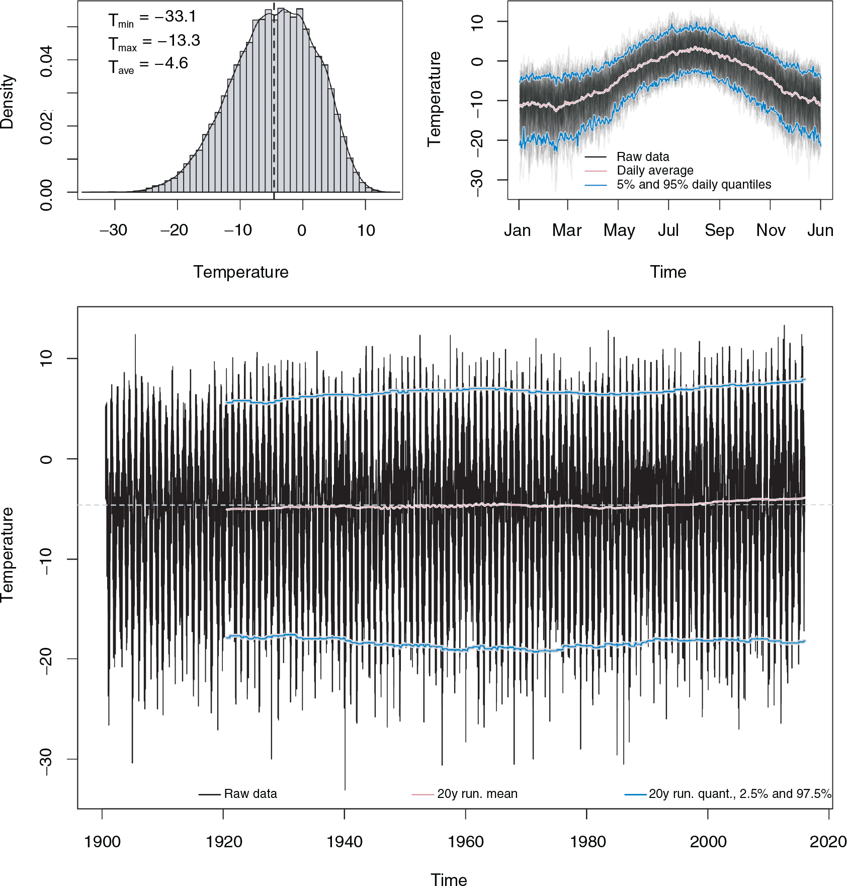
Daily temperature data of the Zugspitze.  The upper-left panel shows a histogram together with a kernel density estimate of the temperature observations.  The upper-right panel shows the raw time series for each year together with empirical mean and quantiles computed for each day of the year.  The lower panel presents the raw time series, including empirical running mean and quantiles computed using a 20-year moving window

In the bottom row of Figure 2, the full temperature time series is shown. Compared to the overall average temperature of − 4 . 6 ∘ C, it seems that after 1980 and between 1920 and 1940 , a temperature increase took place, as indicated by the 20 years, running mean. Between 1940 and 1980 , the running mean fluctuates around its global mean in a more unstructured way. In addition, there is a very small increase in temperature variation over the last 30 years, visible when comparing the 2.5 % and 97.5 % , 20 years running quantiles.

In practice, (temperature) climatology models are oftentimes used for improving probabilistic weather forecasts, for example, by statistical downscaling or as a baseline model for verification. Therefore, it is important to capture the full information of the distribution such that correct inference can be made for all quantities of interest. Therefore, as already suggested from the descriptive data analysis in Figure 2, next to autocorrelation in the observations, subsequent models need to account for complex seasonal patterns, possibly varying over time, as well as varying amounts of fluctuation over season and observation time. Due to the skewness of the response data, a simple Gaussian model is most likely not capable to model all features of the data. Therefore, we exemplify a complex distributional modelling task using three different distributions for daily temperature observations.

2.2 German extreme precipitation

Extreme climatological events play an important role in environmental risk assessment and policymaking. For example, extreme precipitation events can lead to massive flooding and thus cause considerable damage or even fatal accidents. Therefore, the analysis of extreme events has become more and more important in recent years, and a special focus in a modelling context is to capture the tails of the response distribution as accurately as possible. In a distributional regression setting, this oftentimes means that modelling the full response distribution and calculating, for example, the 99 % quantile thereof is not precise enough to estimate the real extreme values. In extreme value theory, an established well-functioning method in such situations is to specify a generalized Pareto ( GP ) model for observations that exceed a certain threshold, that is, a model focusing only on the upper or lower tail of the distribution (Coles, 2001).

In this example, we are interested in extreme 24 -hour precipitation records measured in millimeters in Germany. More precisely, the aim of this analysis is to provide a climatological risk map of Germany of extreme 24 -hour precipitation records that most likely reoccur once within 100 years, which is commonly called the 100 -year return level. Besides, other interesting aspects are if the average risk for such extreme precipitation events is increasing over time and how the risk is changing over the season.

The spatial distribution of meteorological stations in the DWD database is shown in the left panel in Figure 3. OPEN IN VIEWER

Figure 3:

Distribution of available meteorological stations (left panel) fitted generalized Pareto distribution to 24 -hour precipitation records (right panel), that is, the histogram shows the excess of records above the station-wise thresholds

Note that beside the quite dense net of meteorological stations, there is also considerable variation in terms of the sea level. This means that the choice of a suitable threshold for using a GP model can be quite different from station to station, for example, a station on a mountain compared to a station in the next valley. Most commonly, models for extreme 24 -hour precipitation records do not account for this fact and choose one ‘global’ threshold for all stations, usually as low as possible, for example, corresponding to the 99 % quantile (see, e.g., Wang and So, 2016) or selected by inspecting so-called mean residual life plots (Coles, 2001). Considering the data of Germany, selecting one threshold for all stations can lead to a significant dropout of meteorological stations, which can in turn affect prediction quality, especially in regions without measurements. As a strategy to select thresholds, we estimate station-wise models, including a time and seasonal trend, using a grid of threshold values. Beginning with the lowest threshold, the goodness-of-fit in terms of normality of the resulting quantile residuals (see Section 5) is evaluated. If the quantile residuals do not follow a standard normal distribution, the threshold is increased. This procedure is cycled over the grid of thresholds until a suitable value is identified (see, e.g., Zoglat et al., 2014 and Wadsworth and Tawn, 2012 using a similar strategy for threshold selection). Using this procedure, after identifying a suitable threshold for each station, the GP model is fitted using the station-wise subsets of precipitation records that are larger or equal to the thresholds.

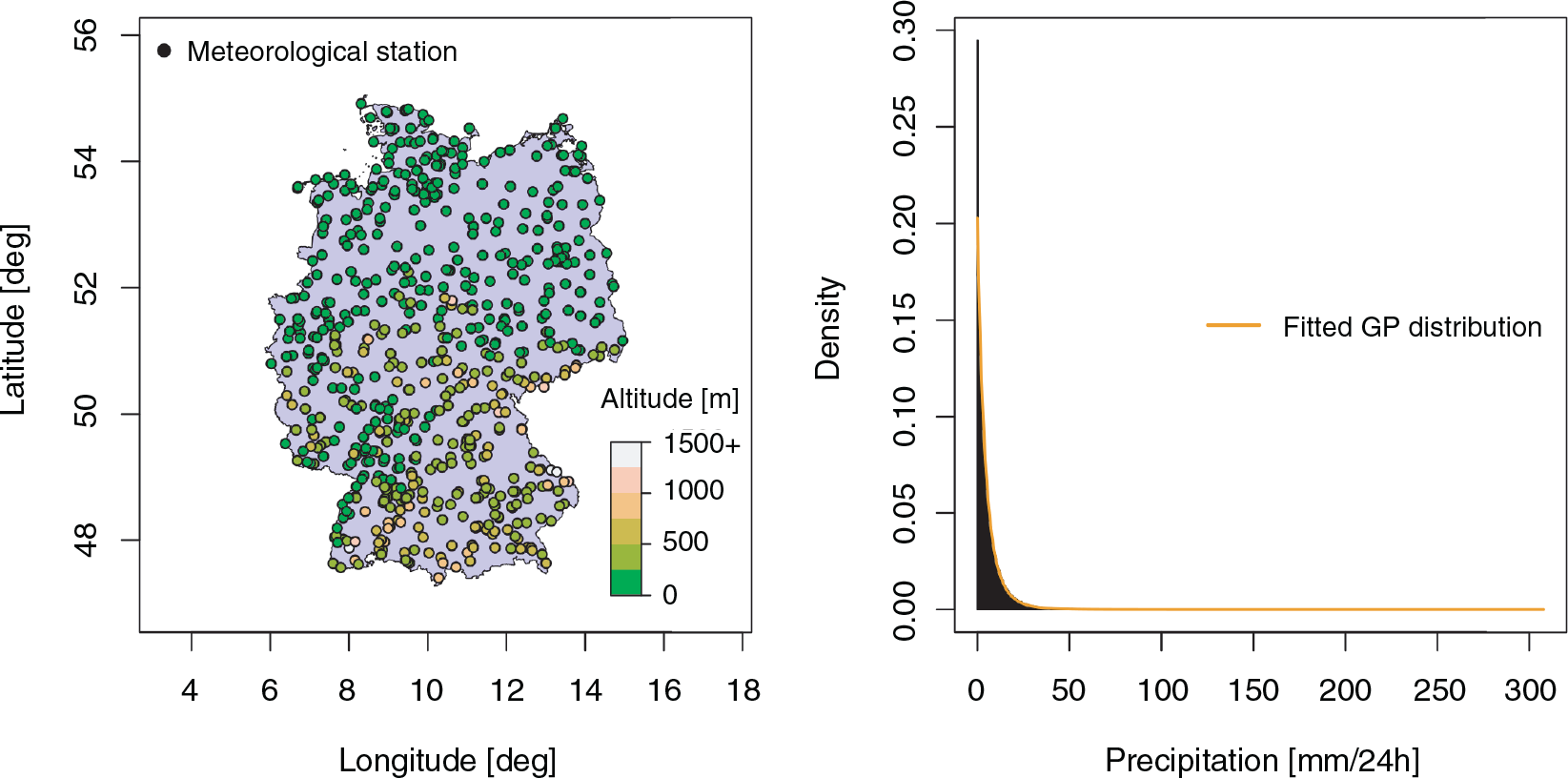
Similarly to the first example, to account for possible time trends in extreme precipitation, it is necessary to use homogenized long-term time series. Therefore, we only used observations of meteorological stations with the highest quality, as reported by the quality flags from the DWD. Additionally, we only analysed data from stations that did not change in altitude more than 10 m. The final dataset consists of 1.138.868 observations of 569 meteorological stations. A histogram of the 24 -hour precipitation records using the selected station-wise thresholds together with a density estimate of a fitted GP model is shown in the right panel of Figure 3.

In this example, note that for example the computation of the mean GP distribution is a transformation of the scale and the shape parameter. This is particularly easy to derive in Bayesian inference based on MCMC simulations.

Most common regression specifications relate the conditional expectation of the response variable of interest y i to a set of explanatory variables (or covariates) x i via

E ( y i | x i ) = h ( η ( x i ) ) , i = 1 , … , n ,

Distributional regression models overcome this limitation and allow for regression effects on potentially all parameters of the response distribution (Rigby and Stasinopoulos, 2005). More specifically, distributional regression assumes that the conditional distribution is of a specific type (e.g., normal, gamma, etc.) with K parameters and that all parameters are associated with a separate regression predictor, that is,

y i | x i ∼ D ϑ 1 ( x i ) , … , ϑ K ( x i ) ,

For relating the different distributional parameters ϑ 1 ( x i ) , … , ϑ K ( x i ) to the covariates, we rely on additive predictors of the form

η i ϑ k = f 1 ϑ k ( x i ; β 1 ϑ k ) + … + f J k ϑ k ( x i ; β J k ϑ k ) ,

To ensure regularization of the functions f j ϑ k ( · ) in the frequentist approach, so-called penalty terms are added to the objective log-likelihood function. The Bayesian analogue are shrinkage priors that are assigned to the regression coefficients, which are commonly based on multivariate normal priors. For more details on prior specifications for smooth terms see, for example, Umlauf et al. (2017).

In analogy to GLMs (Nelder and Wedderburn, 1972), the predictors are then linked to the distributional parameters via known monotonic and twice differentiable response functions h k ( · ) such that

ϑ k ( x i ) = h k η i ϑ k .

OPEN IN VIEWER

Table 1:

Commonly used effect types in distributional regression models

Covariates	Effect Types
	Linear effect x · β
	Linear interaction x 1 · x 2 · β
Scalar covariates (categorical or continuous)	Smooth non-linear effect f ( x )
	Varying coefficient f ( x 2 ) · x 1
	Smooth interaction surface f ( x 1 , … , x L )
Grouping variable s	Random intercept β s
	Spatial effect f ( s )
Grouping and scalar,	Random slope x · β s
time variable t	Space-time effect f ( s , t )
	Functional random intercept f s ( t )

3.1 Models for daily temperatures

In our analysis of the temperature data of the Zugspitze presented in Section 2, the normal distribution T i ∼ N ( μ ( x i ) , σ ( x i ) 2 ) is a natural starting point since temperatures data do not involve natural limits on the domain but have continuous support over the whole real line. Since we are also allowing for regression effects on the variance parameter σ ( x i ) 2 , the distributional normal model already allows us to account for regression effects beyond the mean in the form of covariate-dependent, heteroscedastic variances. However, as illustrated in Section 2.1, there is also some empirical indication that the temperature data exhibit skewness (see Figure 2), which may also change over time such that it makes sense to consider some competing distributional specifications.

We, therefore, work with two alternative, more flexible distributions with distinguished parameters for skewness and kurtosis. More precisely, we consider the Box–Cox t distribution T i ∼ BCT ( μ ( x i ) , σ ( x i ) , ν ( x i ) , τ ( x i ) ) and the Box–Cox Power Exponential (BCPE) distribution T i ∼ BCPE ( μ ( x i ) , σ ( x i ) , ν ( x i ) , τ ( x i ) ) which involve not only a location parameter μ ( x i ) and a scale parameter σ ( x i ) that determine the location and the variability of the distribution but also additional shape parameters ν ( x i ) and τ ( x i ) controlling the skewness and kurtosis of the respective distribution (Rigby and Stasinopoulos, 2004, 2006). Since the support of both distributions is defined only for 0 < y < ∞ , we shifted the temperature observations by c = | T min | + 1 to ensure positiveness. All model predictions for the location parameter μ ( x i ) are then re-transformed by the same constant c . We will later discuss possibilities to compare the fit of these candidate distributions in more detail.

The skewness parameter ν ( x i ) is real-valued such that no response function is required. In contrast, the location μ ( x i ) and scale parameter σ ( x i ) as well as the kurtosis parameter τ ( x i ) have strictly positive support, and we therefore use the exponential response function to ensure this restriction. For simplicity, we treat the kurtosis parameter as a constant ( τ ( x i ) ≡ τ independently of covariates), while for all other parameters, we consider a predictor of the form (note that for better readability we neglect the superscript ϑ k in the upcoming)

η i = β 0 + f 1 ( T i − T i − 1 ) + f 2 ( yday i ) + f 3 ( year i ) + f 4 ( yday i , year i ) , i = 1 , … , 42 414 ,

where i = 1 , … , 42 414 identifies the consecutive days of the observation period. The effects f 1 ( · ) to f 4 ( · ) relate to different types of regression effects chosen to fit with certain stylized features of the data:

Temperature data are temporally correlated, and we therefore include daily temperature differences T i − T i − 1 in the non-linear effect f 1 ( · ) to account for this temporal correlation, assuming that rather the change in temperature than the absolute value is relevant. This way, the time trend is estimated at the correct scale, compared to a model including a lag effect that will absorb part of the trend information, in which we are especially interested in this analysis.

Due to seasonal variation over the year, we include a cyclic trend component based on the day of the year, in f 2 ( · ) which is allowed to vary smoothly over the year, but repeats every year while ensuring that the non-linear effect on 31 December and 1 January are fused together smoothly.

To account for a potential long-term trend in temperatures, we include an overall time trend based on the years from 1900 to 2015 in f 3 ( · ) .

To allow for time variation in the seasonal component, we furthermore include an interaction between day of the year and year in f 4 ( · ) .

3.2 Model for extreme precipitation

For modelling extreme values of precipitation, we rely on the GP distribution P i ∼ GP ( ξ ( x i ) , σ ( x i ) ) , which naturally arises from extreme value theory based on the peak over threshold approach. In this example, we use exponential response functions for both parameters, ξ ( x i ) and σ ( x i ) , as well as the following predictor

η i = β 0 + f 1 ( alt ) + f 2 ( year i ) + f 3 ( yday i ) + f 4 ( lon i , lat i ) + f 5 ( yday i , lon i , lat i ) , i = 1 , … , 1 138 868 ,

where we include the following effects:

Function f 1 ( · ) reflects the natural, potentially non-linear effect of altitude on precipitation.

Similarly to the temperature model, effects f 2 ( · ) and f 3 ( · ) account for a possible long-term time trend as well as seasonal trends of the day of the year.

In addition, to account for spatial variation, we include a spatially correlated effect f 4 ( · ) of longitude and latitude coordinates modelled as a two-dimensional smooth surface.

Moreover, spatial variation might be pronounced for the seasonal trend; therefore, a spatially varying seasonal effect f 5 ( · ) is included as an interaction.

4 Monitoring and convergence of Markov chains

OPEN IN VIEWER

Figure 4:

Trace- and ACF plots generated from the Gaussian daily temperature model.  The samples of one smoothing variance of model term f 4 of the μ parameter are shown in the first column together with a smooth trend line.  The second column shows the corresponding empirical ACF, while the third column visualizes the maximum ACF values over all model parameters.  The upper row illustrates the behaviour of the Markov chain using poor starting values.  The second row shows the effect of using good starting values, for example, generated by a backfitting algorithm.  The bottom row shows samples generated from 8 parallel Markov chains with 6 000 samples, a burn in phase of 2 000 and thinning of 10 for each chain

Let us start with the situation that a fixed model specification is given and we are estimating the model based on MCMC simulations. In this case, it is important to monitor the mixing and convergence behaviour of the underlying Markov chain to avoid that spurious results are obtained. All methods discussed in the following rely on inspecting the posterior samples either based on graphical visualization or certain summary statistics. In the following, we assume some familiarity with the principles of Bayesian inference based on MCMC as provided, for example in Green (2001).

The necessity to monitor the convergence of the Markov chain arises from the fact that MCMC simulations are not optimizing a certain estimation criterion (such as least squares or the log-likelihood) where convergence implies that the estimate of interest converges to the optimal value, but rather we are interested in achieving convergence to the posterior distribution. This unfortunately implies that convergence is way harder to determine in practice, although it is guaranteed from a theoretical perspective under mild regularity conditions. Furthermore, since we are generating a Markov chain, the samples will necessarily exhibit some degree of autocorrelation that has to be taken into account. To illustrate different aspects of monitoring Markov chains in MCMC, Figure 4 contains sampling paths as well as autocorrelation functions (ACFs) for three different scenarios of the estimation process of the daily temperature model of the Zugspitze.

The first row illustrates the behaviour of the Markov chain when starting from a badly chosen starting value. In this case, it takes roughly 300 iterations until the Markov chain has reached the part of the parameter space that is supported by high values of the posterior distribution. This phase is known as the burn in period of MCMC simulations and should be discarded so that results are not impaired by the convergence towards the posterior. Unfortunately, even after the burn in period, the mixing of the Markov chain shown in the first row is far from satisfactory and shows insufficient mixing as demonstrated by the extremely high autocorrelations. To improve mixing and reduce autocorrelations, a common strategy is to apply a thinning strategy where, for example, only every 10th sample is retained. An appropriate thinning value can often be inferred from the autocorrelation function, but in case of the first row in Figure 4, this would result in a really large value such that the MCMC sampler would have to run for a huge number of iterations to obtain a post-thinning sample of appropriate size. Hence, although one may obtain quasi-independent samples by thinning, it is typically more efficient to determine a sample strategy with only moderate dependence already by construction. For example, a highly efficient sampling scheme is to construct approximate full conditionals based on a second-order Taylor series expansion of the log-posterior centred at the last state (see, e.g., Fahrmeir et al., 2004; Umlauf et al., 2017). Moreover, finding good starting values for the MCMC simulations is especially important for smoothing variances of complex model terms, that is, for the spatially varying seasonal effect f 5 ( · ) of the GP model. Therefore, the smoothing variances, as well as regression coefficients, are estimated prior MCMC by a backfitting algorithm with step-wise selection of the smoothing variances (for more details see Umlauf et al., 2017), which is the default using the R package bamlss.

The Markov chain in the second row starts from better initial guesses, and therefore only shows a smaller trend towards the posterior and already considerably reduced autocorrelation. Still, the samples cannot yet be considered as being independent such that an appropriate amount of thinning should be applied. The third row contains samples from eight independent chains after removing a burn in period and after thinning the Markov chain to make the samples approximately independent. The Markov chains do not show any indication of a trend, autocorrelations are very low and repeated runs of the Markov chain produce a similar behaviour. In summary, graphical inspection of the sampling paths and the autocorrelation function provide good guidance on convergence and mixing of the Markov chains with respect to the following aspects: determination of the burn in period, thinning of the Markov chain to make the samples independent and mixing of the Markov chain by comparing different chains.

The major drawback of graphical approaches is that for complex models with hundreds or even thousands of parameters, it is hard to monitor all parameters simultaneously. In this case, it can be useful to rely on convergence diagnostics that can be computed from multiple Markov chains produced for the same model (as implemented in the R package coda, Plummer et al., 2006). The most common approaches are

Gelman and Rubin's convergence diagnostic (Gelman and Rubin, 1992; Brooks and Gelman, 1998),

Similarly, Geweke's diagnostic is testing for convergence based on differences of the mean of the first and last part of the MCMC chains. The test statistic is asymptotically normal distributed, that is, if MCMC chains have converged, differences should be small when quantifying them using a standard Z-score. If the Z-score shows a lack of convergence, it is useful to successively discard more and more samples until the chain is halved in order to identify the iteration from which convergence is achieved. Again, convergence of the MCMC chains of the final BCPE model is achieved according to a conservative 1 % significance level since the resulting Z-values are within boundaries of the 0.5 % and 99.5 % quantile of the standard normal distribution when dividing the chains in half.

Heidelberger and Welch's run length control test is computed by successively discarding samples until either the test is passed or half of the chain has been discarded. In practice, the diagnostic can be used to automatically define an accurate burn in phase for the MCMC chains. When computing, the test for the MCMC chains of the final BCPE model all chains passed the stationarity test.

We now turn our attention to the actual determination of suitable models for an empirical analysis. A common way can be to proceed along the following steps:

Compile a list of potential response distributions: Based on some stylized features of the data and, in particular, the domain of the observed response values, one can often come up with a sensible list of candidate response distributions. For example, in case of the temperature data of the Zugspitze, we are interested in continuous data without any domain restrictions and potentially skewed distributions, while for the precipitation data the peak over threshold approach implied the GP distribution as a suitable model class. Other types of common response structures relate to continuous non-negative responses (e.g., log-normal or gamma distribution), count data (Poisson, negative binomial, zero-inflated Poisson, zero-inflated negative binomial, hurdle models), zero-adjusted responses (log-normal or gamma with an additional spike at zero), fractional responses (beta), etc. A good reference for available distributions in R is the package gamlss (Stasinopoulos and Rigby, 2016) and gamlss.dist (Stasinopoulos et al., 2016), for which package bamlss also provides support.

5.1 Randomized quantile residuals

Randomized quantile residuals (Dunn and Smyth, 1996) are based on the probability integral transform (PIT) that indicates that for a continuous random variable Y with cumulative distribution function F , we have

F ( Y ) ∼ U ( 0 , 1 ) ,

that is, evaluating the cumulative distribution function on the random variable yields a uniform distribution. For discrete random variables, there is a corresponding approximate version. For distributional regression models, one can now replace F with the estimated cumulative distribution function F ̂ = F ϑ ̂ and evaluate it on the observed response values. If the model provides a good approximation of the true data generating mechanism, this should yield a sample of approximately i.i.d. uniform distributed random variables that can be visualized in a PIT histogram (Gneiting et al., 2007). Alternatively, a quantile-quantile (Q-Q) plot can be used to determine deviations of Φ − 1 ( F ( Y ) ) from the standard normal distribution. The main advantage of Φ − 1 ( F ( Y ) ) and the Q-Q plot is that the tails of the distribution can be better visualized, because in a PIT histogram the tails can only be displayed as a function of the bin size. In Figure 5, we demonstrate the use of Q-Q plots for the temperature data of the Zugspitze. Clearly, the mean of the quantile residuals using the normal distribution slightly deviates from zero and the residuals exhibit some skewness. This is also indicated by the corresponding Q-Q plot where for high and low temperatures the quantiles deviate from the diagonal line. Modelling the skewness and kurtosis parameter seems to improve the model fit, the histogram of the residuals of the Box–Cox t model already seems to be more or less symmetric around zero; however, concerning the Q-Q plots, the quantile residuals of the BCPE model seem to follow best a normal distribution, such that the confidence bands computed using all parameter samples almost cover the diagonal over the full range. Therefore, the BCPE model is considered as the best model for the daily temperature data.

OPEN IN VIEWER

Figure 5:

Randomized quantile residuals of the daily temperature models,  The top row shows histograms of posterior mean quantile residuals together with a kernel density estimate; the bottom row shows the resulting quantiles versus the theoretical quantiles of the standard normal distribution.  The small black dots represent the posterior mean quantiles of over all posterior samples, the blue-dashed lines represent the corresponding 95 % credible bands

5.2 Model selection criteria

Quantile residuals and the PIT mostly provide a basic check whether a candidate model provides a reasonably flexible description of the observed data, but they are not well suited to discriminate between rival model specifications in terms of covariate effects. The latter can, for example, be achieved by Bayesian analogues to frequentist information criteria such as Akaike's information criterion (AIC). The most popular approaches are the deviance information criterion (DIC; Spiegelhalter et al., 2002) and the widely applicable information criterion (WAIC; Watanabe, 2010). Both can be easily determined based on the samples for the parameters of a Bayesian model specification and can be interpreted in complete analogy to the AIC (i.e., smaller values indicate a better fit). However, since they are estimated from the data, there is inherent sampling variability such that small differences in the information criteria should not be over-interpreted. Table 2 reports the DIC for the three different models for the daily temperature data of the Zugspitze along with the estimated effective number of parameters (that provide an estimate for the effective dimension of the model). The DIC also clearly favours the BCPE model over the competing approaches, although it is also the model with the largest number of parameters.

OPEN IN VIEWER

Table 2:

Deviance information criterion (DIC) together with estimated effective number of parameters (pd) of the daily temperature models

Model	DIC	pd
N ( μ , σ 2 )	232 426.6	138.7
BCT ( μ , σ , ν , τ )	231 168.1	181.7
BCPE ( μ , σ , ν , τ )	230 938.6	189.7

Note: Accoring the DIC the best model is the BCPE model which is highlighted by the bold text.

When being interested in the predictive ability of distributional regression model, comparing results based on predictive proper scoring rules (Gneiting et al., 2007) can be a valuable alternative. Klein et al. (2015c) provide details on different scores for various types of responses. Basically, the goal of all specifications is to evaluate the predictive ability based on rules that favour honest predictions while simultaneously taking sharpness (i.e., precision) of the prediction into account. To obtain a truly predictive assessment, the scores will usually be evaluated based on a cross-validation approach which makes their computation numerically demanding compared to information criteria and quantile residuals which can be obtained from one single estimation run.

An implementation of the models discussed in the previous sections is provided in the R package bamlss (Umlauf et al., 2017). The main model fitting function is called bamlss(). The most important arguments are

bamlss(formula, family = ”gaussian”, data = NULL,

weights = NULL, subset = NULL, offset = NULL, na.action = na.omit,

transform = NULL, optimizer = NULL, sampler = NULL, results = NULL,

start = NULL, ...)

where the first two lines basically represent the standard model frame specifications (see Chambers and Hastie, 1992). The formula combines the classic Wilkinson and Rogers (1973) symbolic description, used in most standard R regression functions, with the infrastructure for smooth model terms such as s(), te(), ti(), etc., based on recommended R package mgcv, and handling multiple additive predictors using a list of formulas. Similarly, to other flexible model-fitting functions, users can specify their own family objects.

To give an example how to start using bamlss, the GP model for precipitation extremes presented in Section 3.2 can be fitted using the following R code. The R package and the data is loaded with

R> library(”bamlss”)

R> load(”Pmax.rda”)

Note that the file Pmax.rda containing the data Pmax is available in the online supplemental materials. For estimating the model, a formula needs to be specified. In bamlss, each distributional parameter can be modelled in terms of covariate effects. Therefore, we set up a list of formulas, in this case for parameter ξ and σ , where the first formula should contain the response variable, all other formulas should contain the names of the remaining distributional parameters. For the GP model, the formula is given by

R> f <- list(

+ rain2 ˜ s(alt) + s(year) + ti(yday,bs=”cp”) + ti(lon,lat,bs=”tp”) +

+ ti(yday,lon,lat,bs=c(”cp”,”tp”),d=c(1,2)),

+ sigma ˜ s(alt) + s(year) + ti(yday,bs=”cp”) + ti(lon,lat,bs=”tp”) +

+ ti(yday,lon,lat,bs=c(”cp”,”tp”),d=c(1,2))

+ )

The model is then estimated using the default MCMC sampler

R> b <- bamlss(f, family = ”gpareto”, data = Pmax,

+ n.iter = 12000, burnin = 2000, thin = 10)

where we set the number of iteration of the MCMC sampler to 12 000 and remove the first 2 000 samples (the burn in phase). Moreover, we only keep every 10 th sample which is specified by argument thin. The returned object is of class ”bamlss” for which generic extractor functions such as summary(), plot(), predict(), etc., are provided. For example, the posterior mean function based on MCMC samples for parameter ξ of the GP distribution can be computed by

R> p <- predict(b, model = ”xi”, FUN = mean)

where argument FUN can be any function, for example, a function computing credible intervals from the empirical quantiles of the MCMC samples (FUN = quantile).

Estimating models with MCMC sometimes comes at its price in terms of computation time. For example, fitting the precipitation model specified earlier, with over one million observations, on a Linux system with Intel i7-2600 3.40GHz processors takes about 24 hours using bamlss. In practice, to obtain intermediate results before running a full MCMC simulation, the user can optionally only run the default posterior mode optimization function, which takes about 10 hours for the precipitation example. However, note that the computation time using bamlss for such large and complex problems is still quite good and the infrastructures implemented in bamlss support even larger datasets. In general, to overcome the problem of computation time, one may either resort to parallel computing facilities (parallel chains can be started in bamlss), or approximative faster methods like integrated nested Laplace approximations (Rue et al., 2009). The latter, however, is currently restricted to distributions with only one predictor and hence not applicable for distributional regression models involving multiple predictors.

7 Empirical Analyses

7.1 Daily temperature at the Zugspitze

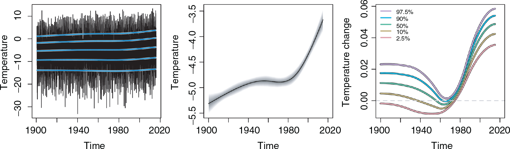
From our previous considerations, we found that the BCPE model provided the best fit for the daily temperature data. Estimated effects of this model are shown in Figure 6. OPEN IN VIEWER

Figure 6:

Estimated effects of the daily BCPE temperature model. About 95 % credible intervals are shown in the middle and bottom row as grey-shaded areas

Note that all effects are shown on the scale of the predictor and all estimates are based on all samples of the MCMC chains. Concerning possible shifts of seasonal variability, as modelled by the time-varying smooth function f 4 ( yday i , year i ) , in the first row of Figure 6, the plots indicate that the two-dimensional effect for parameter μ and σ is not very pronounced and could be dropped in further analyses. Only for the skewness parameter ν , the time variation of the seasonality seems to be more distinct. For the second and third row, additional to the mean effect, the 95 % credible intervals are shown by the grey-shaded areas. For all distributional parameters, the effect of temperature differences T t − T t − 1 is the largest. The effect for parameter μ is increasing for negative differences, that is, if it was warmer at day t − 1 , and is zero for positive differences. The effect for the scale parameter σ is decreasing, that is, uncertainty is increasing if the weather is getting colder. The effect on the skewness parameter ν has a small positive peak for small differences and is about zero for larger differences. The time-trend effect in the last row of Figure 6 is significantly increasing for parameter μ , especially after the year of 1980 . The increase is also significant for parameter σ , indicating higher variation of temperatures. Besides, the effect on the skewness parameter ν is not significant since the 95 % credible intervals cover the zero line over the full time period.

A more detailed picture of the temperature time trend is provided in Figure 7. OPEN IN VIEWER Figure 7:

Estimated mean temperature trends of the daily BCPE temperature model.  The left panel shows the estimated 2.5 %, 10 %, 50 %, 90 % and 97.5 % temperature quantiles of the time trend, blue lines, together with the raw data, black lines.  The middle panel shows the mean time trend together with 95 % credible intervals, grey-shaded area. Estimated slopes of corresponding quantiles are shown in the right panel

The left panel shows estimated mean 2.5 %, 10 %, 50 %, 90 % and 97.5 % temperature quantiles of the BCPE model. When comparing to the 20 years empirical running quantiles in Figure 2, the model seems to nicely adapt to the distribution of the data. The middle panel shows the estimated mean temperature trend together with 95 % credible intervals. The time trend is significantly increasing with a difference of about 1 . 6 ∘ C. To further investigate the change of temperature over time, the right panel of Figure 7 additionally shows the estimated first derivative functions of the 2.5 %, 10 %, 50 %, 90 % and 97.5 % temperature quantiles of the curves presented on the left panel. The plot indicates that the temperatures were increasing in the beginning of the observational period, as indicated by the positive signs of the slope curves. Then, starting at around 1940, until 1980, temperatures were more and more stable as the curves move closer to zero. After 1980, all temperatures are increasing again, and more rapidly compared to the beginning.

7.2 German extreme precipitation

In this example, the aim is to compute a climatological risk map of Germany of extreme 24 -hour precipitation records using the GP distribution, that is, the spatial distribution of 24 -hour records that may occur only once in 100 years. As already mentioned in Section 2.2, this quantity is a transformation of the parameters of the distribution. Using the distributional regression approach in combination with MCMC simulation, it is relatively straightforward to provide correct inference for any desired quantity. This results from the fact that inference is sampling based and, therefore, credible intervals based on quantiles can be computed directly from the transformations.

To provide better insight on the interpretation of the parameters of the GP distribution, Figure 8 shows four example density functions of the GP distribution for varying values of parameter ξ and σ . OPEN IN VIEWER

Figure 8:

Example of GP density functions for varying values of parameters ξ and σ . Higher values of parameter ξ lead to an increase of the probability of extreme events by scaling the density function. Likewise, larger values for the shape parameter σ lead to an increased probability of extreme events by shifting the density function, in this example between 0.1 and 0.2 at y = 0

In the following, the estimated effects for parameter ξ and σ are shown on the logarithmic scale; however, interpretation is similar to Figure 8, that is, positive effects lead to an increase of the probability of extreme precipitation events and negative effects vice versa.

The estimated effects of altitude, the time trend and the seasonal time trend for parameter ξ and σ of the GP model are shown in Figure 9. OPEN IN VIEWER Figure 9:

Estimated effects of altitude, the time trend and the seasonal time trend of the GP model for parameter ξ , top row, and parameter σ , in the bottom row.  The spatially varying seasonal effects are indicated by the coloured lines, the main effects are denoted by the black lines

Note that all effects are visualized using the same scale on the y-axis for the two distributional parameters, such that the comparison of the importance of individual effects is straightforward. The left panels show the effect of altitude. For parameter ξ , the effect seems to be more or less decreasing, that is, considering the tails of the GP distribution, this suggests that in higher altitudes extreme precipitation records become less likely. However, looking at the panel for parameter σ , the effect is strongly increasing until 1 000 m and afterwards about constant, which indicates a strong upward shift of the GP distribution, and hence an increase of extreme 24 -hour precipitation records in higher altitudes. The constant effect for altitudes higher than 1 000  m is most probably caused by the fact that there are too few high altitude meteorological stations available in Germany. The middle panels show the estimated time trends. For both parameters, the trend is basically fluctuating around zero and seems not to have a clear positive or negative direction. The spatially varying seasonal effects in the right panels indicate strong seasonal variation for both parameters, with a peak at around August. Moreover, spatial variation is stronger considering parameter ξ . Especially in the summer months, regions in the north of Germany exhibit higher positive effects on ξ .

The estimated spatial effects for parameter ξ and σ are shown in Figure 10. OPEN IN VIEWER Figure 10:

Estimated spatial effects of the GP model for parameter ξ (left panel) and parameter σ (right panel), respectively

Again note, that the colours are scaled according to the scale of all effects. For example, the spatial effect for parameter ξ is not as pronounced as the corresponding seasonal effect in Figure 9, as indicated by the light red and blue colours. The spatial effect is slightly positive in the southern part of Germany and negative in the north, especially in regions close to the sea. The effect on parameter σ seems to be the other way round; however, especially in the mountainous regions in the Alps and in the Schwarzwald (south east), the effect is clearly positive.

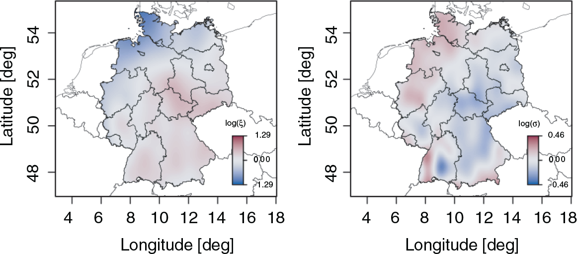
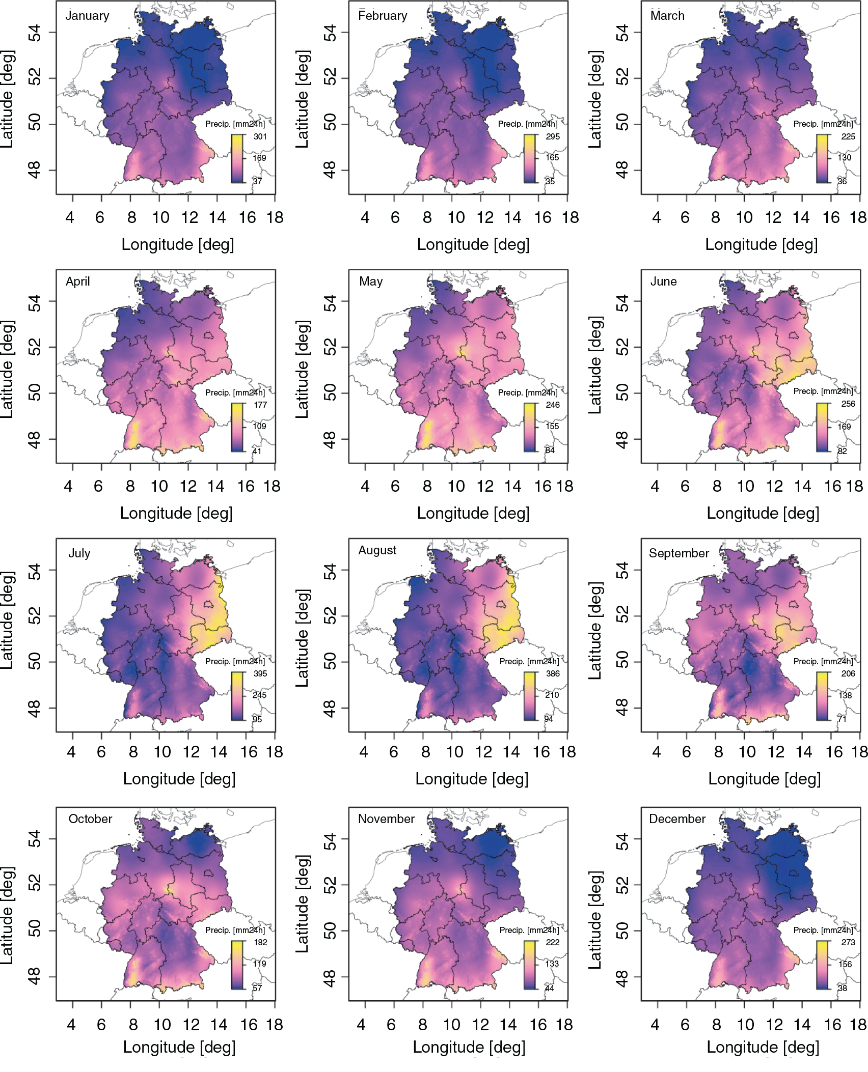
Finally, we computed risk maps for Germany showing estimated 100 -year return levels of 24 -hour precipitation records for each month of the year, Figure 11. OPEN IN VIEWER Figure 11:

Estimated spatial maximum 100 -year return levels of 24 -hour precipitation records (in millimeters) from January to December

As mentioned before, the return levels are a transformation of the estimated parameters of the GP model. Initially, the return levels are calculated for each day of the year and afterwards, the maximum for each month is computed. The maps nicely depict the spatial variation of precipitation over the year, with highest risk of very extreme events in the summer months. Note that each map has its own scaling, otherwise the maps are difficult to interpret because the summer months exceed the winter month by a large amounts over a quite wide area. One interesting aspect is that the risk is highest in the north east of Germany between June and September. This is in line with the observations, the highest 24 -hour record with 321 mm was measured in Zinnwald-Georgenfeld which is located at the border of Germany in the south of the city Dresden.

Distributional regression models, as described in this tutorial, are a flexible extension of GAMs (Wood, 2006; Ruppert et al., 2003; Fahrmeir et al., 2013a) that allow to apply flexible, additive predictor structures not only on the mean but on potentially all parameters of even complex response distributions. This idea has been introduced in a penalized likelihood context by Rigby and Stasinopoulos (2005) as GAMLSS and transferred to a Bayesian context in Klein et al. (2015b,c). We prefer the notion of distributional regression over GAMLSS since in many distributions the parameters are not or only indirectly related to location or scale of the distribution.

The main competitor to distributional regression in applied regression analyses is quantile regression, as also discussed in Waldmann (2018) which is also part of this special issue. While the main advantage of quantile regression is that one can avoid an explicit distributional assumption for the response distribution, it also alleviates the danger of model misspecification. On the other hand, quantile regression requires strictly continuous responses (i.e., discrete or mixed discrete-continuous responses are not allowed), while distributional regression provides a convenient framework for continuous, discrete and mixed discrete-continuous distributions. Furthermore, quantile regression typically faces the risk of quantile crossing while distributional regression provides a coherent estimate for the complete distribution of the response. A final advantage of distributional regression is that it also facilitates the consideration of multivariate response structures (Klein et al., 2015a; Klein and Kneib, 2016).

Another strategy to gain information of the full response distribution is to use conditional transformation models (Hothorn et al., 2014), which directly model the distribution function using regularized transformation functions. Despite their theoretical attractiveness, these models can quickly become computationally expensive, especially in cases where a number of explanatory variables directly interact with the distribution function. A non-technical introduction of Hothorn (2018) is also part of this special issue.

In addition, variable selection in distributional regression is an important aspect. A well-established strategy is to use boosting algorithms, an introduction is provided within this special issue by Mayr and Hofner (2018).

Considering Bayesian approaches to distributional regression based on MCMC simulations is particularly attractive not only due to its flexibility but also due to the virtues of sampling-based inference. MCMC provides samples for all parameters of the distributional regression model which can be transferred to samples for any quantity of interest that depends on these parameters. In our application on extreme precipitation values, one such quantity was the 100-years return level. Based on samples from these return levels, one can determine point estimates as well as credible intervals without requiring asymptotic considerations.

A particular challenge of distributional regression is the interpretation of results, which often can no longer be achieved in a ceteris paribus-type fashion. As a consequence, designing scenarios of interest for which covariate effects can be evaluated in combination with carefully chosen visualization tools is extremely important. In the future, we will work on making such graphical tools more broadly available and easily accessible.

Acknowledgments

We thank two anonymous referees for their valuable comments that led to a significant improvement of the article. Financial support from the German Research Foundation (DFG) grant KN 922/4-2 is gratefully acknowledged.