A penalized approach for the bivariate ordered logistic model with applications to social and medical data

Abstract

Bivariate ordered logistic models (BOLMs) are appealing to jointly model the marginal distribution of two ordered responses and their association, given a set of covariates. When the number of categories of the responses increases, the number of global odds ratios to be estimated also increases, and estimation gets problematic.

In this work we propose a non-parametric approach for the maximum likelihood (ML) estimation of a BOLM, wherein penalties to the differences between adjacent row and column effects are applied. Our proposal is then compared to the Goodman and Dale models. Some simulation results as well as analyses of two real data sets are presented and discussed.

Keywords

Dale model bivariate ordered logistic model penalized maximum likelihood estimation ordinal association

1 Introduction

Models for association play a central role in ordered categorical data analysis. For the multivariate case, marginal models (MMs) represent a natural choice to model marginal distributions of the responses given covariates. An example of full likelihood-based MM is Dale, 1986. A similar model, the multivariate logistic model described in (Glonek and McCullagh, 1995), but restricted to the bivariate ordered version, is the basis on which we develop our proposal. Some open, or at least not completely solved, problems about estimation of a multivariate ordered logistic model are of computational type and concern maximum likelihood (ML) estimation by iterative algorithms, often providing invalid estimates at the $k$ th step, exceeding the boundaries of the parameter space. Some of such problems could be solved as in (Colombi and Forcina, 2001) and (Bartolucci and Forcina, 2002) by including strict inequality constraints. However, constrained ML estimation is appealing only when a particular application implies natural ordering constraints. On the contrary, when the ordering is not fully reliable, or externally imposed, like in responses which arise from discretized versions of latent continuous variables, using strict inequality constraints may not be appropriate. Indeed, due to lack of subject-matter knowledge that yields natural restrictions on marginal distributions, the use of more flexible approaches would be more helpful and suitable. In these situations, a non-parametric approach may be useful (Dardanoni and Forcina, 1998). Within the possible range of non-parametric approaches, penalization is the one considered in this article. Surprisingly, there is little literature on penalization applied to MMs. (Desantis et al. 2008) apply a ridge penalty to a latent class model for ordinal data to stabilize ML estimation, that would otherwise not be computationally feasible without application of strict constraints. Other contributions deal mainly with forms of longitudinal (Gieger, 1997; Fahrmeier et al., 1999) or horizontal (Bustami et al., 2001) non-parametric modelling. The former focuses on smoothing of variation of marginal and association parameters over time, the latter refers to a form of smoothing on covariates, often by using splines.

Our proposal is based on a form of vertical smoothing, that is across response levels, of the regression parameters in order to regularize the parameter space and/or fit polynomial models using scores ‘chosen by the data’. After recalling the Dale, the Gloneck–McCullagh and the bivariate partial proportional odds models, Section 2 introduces the penalized ML estimation approach and the penalty terms we propose. Section 3 deals with hypothesis testing and the asymptotic distribution of the penalized log-likelihood ratio test. The theoretical results of Section 3 and the performance of the approach is shown by simulation in Sections 4–5. Two applications are considered in Section 6: In the first one, we compare our proposal to the Dale (1986) and Goodman (1979) models on a literature dataset on social mobility, whereas the second application is about the analysis of a dataset of liver disease patients.

2 Bivariate ordered logit models

For two ordered outcomes $A_{1}$ and $A_{2}$ , define the row and column marginal cumulative probabilities of a $D_{1} \times D_{2}$ contingency table $A_{1} A_{2}$ as

μ_{r .} = P (A_{1} \leq r) = \sum_{i \leq r} π_{i .}, μ_{. c} = P (A_{2} \leq c) = \sum_{j \leq c} π_{. j},

and the upper-left quadrant probabilities as

\begin{matrix} μ_{rc} = P (A_{1} \leq r, A_{2} \leq c) & = & \sum_{i \leq r} \sum_{j \leq c} π_{ij}, \end{matrix}

with $r = 1, \dots, D_{1}, c = 1, \dots, D_{2}$ . By differencing we obtain

\begin{matrix} P (A_{1} \leq r, A_{2} > c) & = & μ_{r .} - μ_{rc}, \\ P (A_{1} > r, A_{2} \leq c) & = & μ_{. c} - μ_{rc}, \\ P (A_{1} > r, A_{2} > c) & = & 1 - μ_{r .} - μ_{. c} + μ_{rc} . \end{matrix}

By choosing the cumulative odds as ordinal risk measures, and the logit as link function, we obtain the global logits (or log global odds):

\begin{matrix} \log ϕ_{1 r} & = & logit [P (A_{1} \leq r)] = \log (μ_{r .}) - \log (1 - μ_{r .}), \end{matrix}

(2.1)

\begin{matrix} \log ϕ_{2 c} & = & logit [P (A_{2} \leq c)] = \log (μ_{. c}) - \log (1 - μ_{. c}), \end{matrix}

(2.2)

$r = 1, \dots, D_{1} - 1, c = 1, \dots, D_{2} - 1$ . By choosing the cross-products of quadrant probabilities as ordinal association measures, and the natural logarithm as link function, the log global odds ratios (or log-GORs) are defined as:

\begin{matrix} \log ψ_{rc} & = & \log \frac{P (A_{1} \leq r, A_{2} \leq c) P (A_{1} > r, A_{2} > c)}{P (A_{1} \leq r, A_{2} > c) P (A_{1} > r, A_{2} \leq c)} \\ = & \log \frac{μ_{rc} (1 - μ_{r .} - μ_{. c} + μ_{rc})}{(μ_{r .} - μ_{rc}) (μ_{. c} - μ_{rc})} . \end{matrix}

(2.3)

Given the three parameters $μ_{r .}$ , $μ_{. c}$ and $ψ_{rc}$ , we may find the corresponding joint cumulative probabilities with the following inversion formula:

\begin{matrix} μ_{rc} = \{\begin{matrix} \frac{1}{2} (ψ_{rc} - 1)^{- 1} (a_{rc} - \sqrt{a_{rc}^{2} + b_{rc}}) & if ψ_{rc} \neq 1, \\ μ_{r .} μ_{. c} & if ψ_{rc} = 1, \end{matrix} \end{matrix}

(2.4)

where $a_{rc} = 1 + (μ_{r .} + μ_{. c}) (ψ_{rc} - 1)$ and $b_{rc} = - 4 ψ_{rc} (ψ_{rc} - 1) μ_{r .} μ_{. c}$ . If the cumulative probabilities $μ_{r .}$ and $μ_{. c}$ satisfy the constraints $μ_{r .} < μ_{r + 1, .}$ for $r = 1, \dots, D_{1} - 1$ , and $μ_{. c} < μ_{., c + 1}$ for $c = 1, \dots, D_{2} - 1$ , and the global odds ratios are not dependent on the category, that is, $ψ_{rc} = ψ$ , then (2.4) is a Plackett distribution (Plackett, 1965). Thus, the bivariate Dale regression model for $(ϕ_{1}, ϕ_{2}, ψ_{12})^{'}$ is defined as:

\{\begin{matrix} \log [ϕ_{1, r} (x)] = β_{10 r} - β_{1}^{'} x, \\ \log [ϕ_{2, c} (x)] = β_{20 c} - β_{2}^{'} x, \\ \log [ψ_{rc} (x)] = α + ρ_{1 r} + ρ_{2 c} + σ_{rc} - β_{3}^{'} x, \end{matrix}

(2.5)

$r = 1, \dots, D_{1} - 1, c = 1, \dots, D_{2} - 1$ . This model does not require marginal scores for responses, and it is also invariant under any monotonic transformation of the marginal responses. Further, since the model is based on global odds ratios, collapsing adjacent row or column categories does not produce any effect in parameter interpretation, which remains unchanged with the exception of the intercepts related to the collapsed categories. This is in contrast with the RC Goodman model which uses local cross-ratios. In a more general framework than (2.5), Glonek and McCullagh (1995) introduce the multivariate logistic model:

C^{'} \log (L π) = X β,

(2.6)

where $C$ is a contrasts matrix, $L$ is a matrix with elements $a_{ij} \geq 0$ such that $L π = μ$ , $η = C^{'} \log (L π)$ is the parameter vector of interest, and $X$ , an $n \times p$ matrix, with $n = \prod_{k = 1}^{K} D_{k}$ . Although formulation (2.6) is referred to $K \geq 2$ responses, here only two responses $A_{1}$ and $A_{2}$ are considered. The components of $C^{'} \log (L π)$ are symbolically denoted by $(η_{\emptyset}, {η^{'}}_{A 1}, {η^{'}}_{A 2}, {η^{'}}_{A 1 A 2})$ , where $η_{\emptyset} = \log (Σ π) = 0$ is the null contrast and the remaining vectors have elements specified by (2.1), (2.2) and (2.3), respectively. We will refer to (2.6) as the bivariate ordered logistic model (BOLM). Lapp et al. (1998) show how to fit the Dale and Goodman models starting from the framework of a BOLM. Some computational problems may arise when fitting a multivariate logistic model, depending on the number of responses and categories. For example, when inverting equation $η = C^{'} \log (L π)$ to obtain $π$ in terms of $η$ , it may happen that for certain fixed values of $η$ no positive solution $π$ exists. Although $π > 0$ ensures the matrix $C^{'} D^{- 1} L$ to be invertible (Glonek and McCullagh, 1995, Theorem 1), where $D = diag (L π)$ , the range of the mapping is not a hyper-rectangle and fixing some components of $η$ restricts the range of the remaining components, that is, the model is not variation independent. Although this problem is particularly magnified for $K > 2$ responses (Bergsma and Rudas, 2002; Qaqish and Ivanova, 2006), computational problems can also arise in the bivariate case, above all when considering certain particular model configurations. For instance, it may happen that not only the intercepts but some covariates have a category-dependent effect. To highlight this effect one may want to fit a bivariate version of the partial proportional odds model proposed by Peterson and Harrell (1990). However, such a model can be computationally very hard to fit, even with a limited and reasonable number of parameters. To deal with this difficulty, we propose to regularize the parameter space by penalizing the log-likelihood of the model. This allows to increase the range of possible models to be fitted. The penalty term we use for this is introduced in Section 2.1.

The fit of a BOLM becomes computationally hard also when the number of response categories increases. In addition, the model may result overparameterized. Lapp et al. (1998) fit a Dale model by imposing constraints on the row and column interactions of the association intercepts in order to reduce the number of parameters. However, this type of data appears to be too ‘rich’ to be modelled with fully parametric models and non-parametric or semiparametric models, followed by graphical presentation, could result more useful (Eilers and Marx, 1996). In order to smooth the marginal and association effects across the response categories, in Section 2.2, a penalty term for non-parametric modelling is introduced. Such term, often employed in the P-spline context (Eilers et al., 2006), has been suitably re-written to be used in the framework of a BOLM. In part, this approach can be considered the bivariate extension of the models proposed by Tutz (2003).

The ordinal nature of the responses imposes inequality constraints on marginal distributions which have to be taken into account in model estimation. In Section 2.3, we present a penalty term, which is able to mimic such inequality constraints.

In order to better understand the potential of the penalization approach, some further notation is needed, according to that used in Tutz and Scholz (2003) for the univariate cumulative logistic regression model. Let $Q$ be the set of indices of all the covariates, excluding the intercepts, and $P \subset Q$ be a subset of $p$ covariates. Let $S$ be the set of indices of the variables whose effects we assume do not depend on categories and such that $S \subseteq P$ , and let $\bar{S} = P ∖ S$ . In particular, we define $S$ and $\bar{S}$ as $S = \cup_{k = 1}^{3} S_{k}$ and $\bar{S} = \cup_{k = 1}^{3} {\bar{S}}_{k}$ , where $S_{k}$ and ${\bar{S}}_{k}$ are the subsets of $S$ and $\bar{S}$ , respectively, associated to the $k$ th equation. To complete the notation, let $S^{0} = {0} \cup S$ and ${\bar{S}}^{0} = {0} \cup \bar{S}$ . Consider the following model where only a part of the covariates is supposed to be category independent:

{\begin{array}{l} \log [\emptyset_{1 r} (x_{i})] = β_{10 r} + {β^{'}}_{1 S_{1}} x_{i S_{2}} + β_{1 {\bar{S}}_{1} r} x_{i {\bar{S}}_{1}}, \\ \log [\emptyset_{2 C} (x_{i})] = β_{20 c} + {β^{'}}_{2 S_{2}} x_{i S_{2}} + β_{2 {\bar{S}}_{2} c} x_{i {\bar{S}}_{2}}, \\ \log [Ψ_{r c} (x_{i})] = β_{30 r c} + {β^{'}}_{3 S_{3}} x_{i S_{3}} + β_{3 {\bar{S}}_{3} r c} x_{i {\bar{S}}_{3}}, \end{array}

(2.7)

$(r = 1, \dots, D_{1} - 1, c = 1, \dots, D_{2} - 1)$ . We refer to model (2.7) as the Non-Uniform association and tially Proportional Odds Model (NUPPOM). Although in the univariate case, the phrase ‘proportional odds’ is usually referred to a model with covariate effects which do not depend on the categories, here we will refer to a Uniform association and Proportional Odds Model (UPOM) as a model defined from (2.7) assuming $β_{30 rc} = β_{30}$ and $\bar{S} = \emptyset$ . On the other hand, a Non-Uniform association and Non-Proportional Odds Model (NUNPOM) will be defined from (2.7) assuming $S = \emptyset$ and with category-dependent association intercepts. Note that the intercepts for the marginal equations (i.e., the global logit intercepts) are never supposed to be independent of the categories, whatever the model. According to these definitions, the bivariate Dale model (2.5) is a NUPOM, and it becomes a UPOM when $ρ_{1 r} = 0$ , $ρ_{2 c} = 0$ and $σ_{rc} = 0$ , $r = 1, \dots, D_{1} - 1, c = 1, \dots, D_{2} - 1$ . Further, to specify that a NUPPOM is fitted we will also write $NUPPOM (S)$ and to indicate that a UPOM is fitted we will also write $UPOM ({\bar{S}}^{0})$ .

\indent Under multinomial sampling with frequencies $y_{i} \sim M (n_{i},$ $π_{i})$ , consider the model $C^{'} \log (L π_{i}) = X_{i} β$ , with the matrices $C$ and $L$ such that the marginal pameters are global logits, the association pameters are log global odds ratios, and the constraint $\sum_{j = 1}^{D_{1}} \sum_{k = 1}^{D_{2}} π_{ijk} = 1$ is included. Then, the kernel of the log-likelihood is

l (β) = \sum_{i = 1}^{m} l (β; y_{i}) = \sum_{i = 1}^{m} y_{i}^{'} \log (π_{i}),

(2.8)

where $m$ , the observed number of response configurations, is such that $\sum_{i = 1}^{m} n_{i} = n$ , with $n$ indicating the sample size. The penalized log–likelihood has the form

l_{P} (β) = l (β) - \frac{1}{2} τ (β),

(2.9)

where $τ (β) = β^{'} P β$ , and $P$ represents the penalization and includes the smoothing ameter. Penalized ML estimation formulas are given and discussed in Appendix A, while Appendix B shows the matrix form of $P$ .

2.1 Penalty terms for ameter space regularization

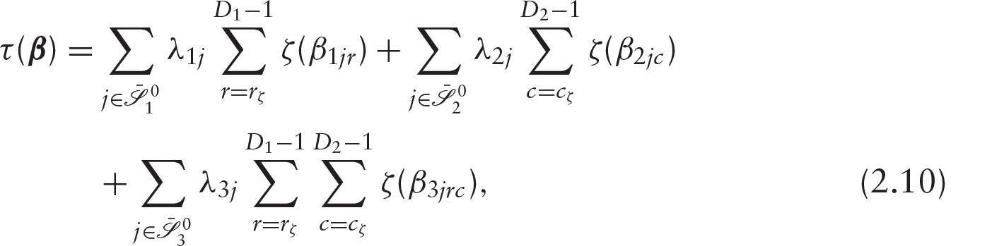
When the cross-tabulation of the responses contains one or more zeros, ameter estimation by Fisher scoring may be challenging at each iteration. In these cases, one may try to reduce $l_{step}$ , the step length (see Appendix A). However, estimates of the association structure may result to be too irregular, with very high (or very low) estimated odds ratios in correspondence of the cell with zeros. In order to stabilize the ML estimates of the BOLM using Fisher scoring, a reduction of the ameter space may be helpful. We propose to penalize both the marginal and the association ameters. In addition, since the model is not variation independent, applying a penalty term on association pameters might be useful to limit the range of the possible values that the marginal pameters can assume, so avoiding a failure of the Fisher scoring. The general expression of $τ (β)$ is:

\begin{matrix} τ (β) & = & \sum_{j \in {\bar{S}}_{1}^{0}} λ_{1 j} \sum_{r = r_{ζ}}^{D_{1} - 1} ζ (β_{1 jr}) + \sum_{j \in {\bar{S}}_{2}^{0}} λ_{2 j} \sum_{c = c_{ζ}}^{D_{2} - 1} ζ (β_{2 jc}) \\ + \sum_{j \in {\bar{S}}_{3}^{0}} λ_{3 j} \sum_{r = r_{ζ}}^{D_{1} - 1} \sum_{c = c_{ζ}}^{D_{2} - 1} ζ (β_{3 jrc}), \end{matrix}

(2.10)

where $λ_{kj}$ is the smoothing ameter for the $j$ th variable of the $k$ th equation of system (2.7), $k = 1, 2, 3$ , and $ζ (\cdot)$ is a generic function that characterizes the penalty term. Notice that the starting values $r_{ζ}$ and $c_{ζ}$ of the summation indices depend on $ζ (\cdot)$ . In the following subsections, we introduce three different specifications of $ζ (\cdot)$ .

2.1.1 The ARC1 penalty term

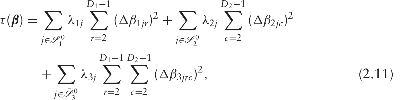
A first specification of $ζ (\cdot)$ is $ζ (α_{t}) = (Δ α_{t})^{2}$ , where $Δ$ is the order 1 difference operator, that is, $Δ α_{t} = α_{t} - α_{t - 1}, t \geq 2$ . This penalty term involves the differences of adjacent row and column pameters (ARC1). The term is defined as

\begin{matrix} τ (β) & = & \sum_{j \in {\bar{S}}_{1}^{0}} λ_{1 j} \sum_{r = 2}^{D_{1} - 1} (Δ β_{1 jr})^{2} + \sum_{j \in {\bar{S}}_{2}^{0}} λ_{2 j} \sum_{c = 2}^{D_{2} - 1} (Δ β_{2 jc})^{2} \\ + \sum_{j \in {\bar{S}}_{3}^{0}} λ_{3 j} \sum_{r = 2}^{D_{1} - 1} \sum_{c = 2}^{D_{2} - 1} (Δ β_{3 jrc})^{2}, \end{matrix}

(2.11)

and it is aimed at overcoming estimation problems by reducing ameter space. As $λ_{kj} \to \infty, k = 1, 2, 3, \forall j \in {\bar{S}}_{k}^{0}$ , all the pameters indexed by $j$ will tend to be equal among the categories. In practice, if all category dependent pameters are involved in the penalization, the model will tend to a UPOM for high smoothing values. Although (2.14) allows to penalize marginal intercepts, it is preferable to avoid a strong penalization on such ameters, in order not to violate (2.15).

The choice of $λ$ is two steps: The first step is based on the minimum value $λ_{\min}$ for which Fisher scoring does not fail. The simulation study in Section 5 will clarify this choice. In the second step, the search of an optimal $λ$ , say $λ_{opt}$ , satisfying criteria such as the Akaike Information Criterion (AIC) or the Bayesian Information Criterion (BIC), is then performed on the interval $[λ_{\min}, + \infty)$ .

2.1.2 Ridge-type penalty

Another specification of $ζ (\cdot)$ aimed at reducing the ameter space is $ζ (α) = α^{2}$ , corresponds to a ridge-type penalty for the bivariate logistic regression model:

\begin{matrix} τ (β) & = & \sum_{j \in {\bar{S}}_{1}^{0}} λ_{1 j} \sum_{r = 1}^{D_{1} - 1} β_{1 jr}^{2} + \sum_{j \in {\bar{S}}_{2}^{0}} λ_{2 j} \sum_{c = 1}^{D_{2} - 1} β_{2 jc}^{2} \\ + \sum_{j \in {\bar{S}}_{3}^{0}} λ_{3 j} \sum_{r = 1}^{D_{1} - 1} \sum_{c = 1}^{D_{2} - 1} β_{3 jrc}^{2} . \end{matrix}

(2.12)

For $λ_{kj} \to \infty, k = 1, 2, 3, \forall j \in {\bar{S}}_{k}^{0}$ , all pameters indexed by $j$ will tend to zero. A similar penalty, not involving the third term, is used by Desantis et al. (2008) in a penalized latent class model for ordinal data.

2.1.3 Lasso-type penalty

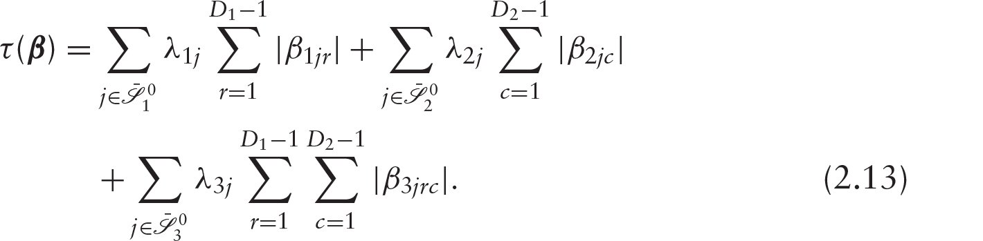
In this article, emphasis for regularization problems is on ARC1, but many other penalty terms are possible. For example, a ‘horizontal’ lasso-type penalization is written as

\begin{matrix} τ (β) & = & \sum_{j \in {\bar{S}}_{1}^{0}} λ_{1 j} \sum_{r = 1}^{D_{1} - 1} | β_{1 jr} | + \sum_{j \in {\bar{S}}_{2}^{0}} λ_{2 j} \sum_{c = 1}^{D_{2} - 1} | β_{2 jc} | \\ + \sum_{j \in {\bar{S}}_{3}^{0}} λ_{3 j} \sum_{r = 1}^{D_{1} - 1} \sum_{c = 1}^{D_{2} - 1} | β_{3 jrc} | . \end{matrix}

(2.13)

For $λ_{kj} \to \infty, k = 1, 2, 3, \forall j \in {\bar{S}}_{k}^{0}$ , all the pameters indexed by $j$ will tend to zero. The lasso penalty may be used as an alternative to (2.15).

A further specification of $ζ (\cdot)$ could be $ζ (α_{t}) = | Δ α_{t} |$ , and $r_{ζ} = c_{ζ} = 2$ , a ‘vertical’ lasso-type penalty on the differences of adjacent ameters, as an alternative to (2.14).

2.2 A penalty term for non-ametric modelling

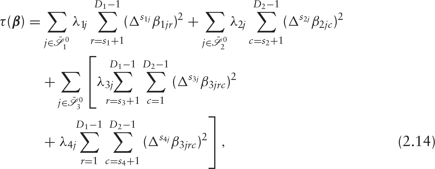
Beside being useful for reducing the ameter space and for reproducing a $UPOM$ , the following generalization of the penalty term ARC1, hereafter denoted by ARC2, can be used to specify row or column effects and to fit non-ametric models where the effects are determined by a polynomial:

\begin{matrix} τ (β) & = & \sum_{j \in {\bar{S}}_{1}^{0}} λ_{1 j} \sum_{r = s_{1} + 1}^{D_{1} - 1} (Δ^{s_{1 j}} β_{1 jr})^{2} + \sum_{j \in {\bar{S}}_{2}^{0}} λ_{2 j} \sum_{c = s_{2} + 1}^{D_{2} - 1} (Δ^{s_{2 j}} β_{2 jc})^{2} \\ + \sum_{j \in {\bar{S}}_{3}^{0}} [λ_{3 j} \sum_{r = s_{3} + 1}^{D_{1} - 1} \sum_{c = 1}^{D_{2} - 1} (Δ^{s_{3 j}} β_{3 jrc})^{2} \\ + λ_{4 j} \sum_{r = 1}^{D_{1} - 1} \sum_{c = s_{4} + 1}^{D_{2} - 1} (Δ^{s_{4 j}} β_{3 jrc})^{2}], \end{matrix}

(2.14)

where $Δ^{a} = Δ (Δ^{a - 1})$ . Consider the following penalty settings:

as $λ_{hj} = 0, h = 1, \dots, 4, \forall j \in {\bar{S}}^{0}$ , an unrestricted model will be fitted;

as $λ_{hj} \to \infty, h = 1, \dots, 4, \forall j \in {\bar{S}}_{1} \cup {\bar{S}}_{2} \cup {\bar{S}}_{3}^{0}$ and $s_{hj} = 1$ , the fitted pameters will tend to be equal, and the model will tend to a $UPOM$ ;

as $λ_{3 j} \to \infty$ , $λ_{4 j} = 0, \forall j \in {\bar{S}}_{3}^{0}$ and $s_{3 j} = 1$ , a model with column effects will be fitted;

as $λ_{3 j} = 0$ , $λ_{4 j} \to \infty, \forall j \in {\bar{S}}_{3}^{0}$ and $s_{4 j} = 1$ , a model with row effects will be fitted;

as $λ_{hj} \to \infty, h = 1, 2, \forall j \in {\bar{S}}^{0}$ and $s_{hj} > 1$ , the fitted pameters will follow a polynomial curve of degree $s_{hj} - 1$ .

as $λ_{hj} \to \infty, h = 3, 4, \forall j \in {\bar{S}}^{0}$ and $s_{hj} > 1$ , the fitted pameters will follow a polynomial surface of degree $s_{3 j} + s_{4 j} - 2$ .

Notice the difference between the penalty terms included in (2.14) and those included in the penalized log-likelihood (14) in Tutz (2003), suggested for a single-ordered response. In that article, the author proposed to penalize the differences of adjacent categories, for a vertical smoothing, jointly to the use of penalized B-splines for a horizontal smoothing, resulting in a form similar to (2.14). Also notice the differences with the bivariate horizontal smoothing approach by Bustami et al. (2001) which presented the additive bivariate Dale model, for continuous, category-independent covariates, as a natural extension of the generalized additive model (Hastie and Tibshirani, 1990).

Penalty (2.14) may be useful to assume certain dependence structures on the categories, for both marginal and association ameters. For example, if one wants to assume a linear trend for the row marginal effects, one may assume $η_{1 ir} = β_{10 r} + \sum_{j = 1}^{p} x_{ij} β_{1 jr}$ , where $β_{1 jr} = α_{0 j} + α_{1 j} δ_{jr}$ , with $α_{0 j}$ and $α_{1 j}$ unknown ameters, and with scores $δ_{jr}$ . In spite of its simplicity, such an approach assumes arbitrary scores. An alternative way is just to use a penalization approach with penalty term ARC2 which uses scores ‘chosen by the data’ (Tutz and Scholz, 2003). Indeed, the smoothing pameters and the polynomial degrees can be chosen on the basis of some criterion, such as the values that minimize the AIC. As a special case, suppose to want to fit a model which assumes a linear trend for the marginal pameters and an association structure composed by the interaction of two first-degree polynomials (The degree of a two-variable polynomial is defined as the highest degree of its terms, and the degree of a term is the sum of the exponents of the variables that appear in it. Since (2.14) allows to fit only polynomial models with interactions, to distinguish each of the possible models having the same degree, it is more practical for us to indicate a model by specifying both the degrees of the one-variable polynomials, omitting to specify the (implicit) presence of interaction terms). By assuming, for simplicity, that the same variable $x_{j}$ is present in all the equations of system (2.7), choosing $s_{hj} = 2, h = 1, \dots, 4$ and high smoothing values, for instance $10^{8}$ , the predictor becomes

$x_{ij} β_{jr} = x_{ij} γ_{01 j} + x_{ij} (γ_{11 j} \cdot r)$

$x_{ij} β_{jc} = x_{j} γ_{02 j} + x_{ij} (γ_{12 j} \cdot c)$

$x_{ij} β_{jrc} = x_{ij} γ_{03 j} + x_{j} (γ_{13 j} \cdot r) + x_{ij} (γ_{23 j} \cdot c) + x_{ij} (γ_{33 j} \cdot r \cdot c)$ ,

with scores $δ_{jr} = r, δ_{jc} = c$ and $δ_{jrc} = (r, c)^{'}$ , that is, pre-assigned equally spaced scores.

2.3 Mimicking inequality constraints

The ordinal nature of the responses introduces some explicit ordering constraints on marginal distribution which have to be taken into account to avoid ill-conditioning of the predictor space. In ticular, for the $i$ th individual, such constraints are on the marginal predictors, that is,

β_{k 01} + β_{k 1}^{'} x_{i} < β_{k 02} + β_{k 2}^{'} x_{i} < \dots < β_{k 0, D_{k} - 1} + β_{k, D_{k} - 1}^{'} x_{i},

(2.15)

k = 1, 2 .

Although Lagrangians can be used to take into account such constraints, in the spirit of this article, a penalized-oriented solution could be the following:

τ (β) = \sum_{i = 1}^{n} [\sum_{k = 1}^{2} λ_{k} \sum_{r = 2}^{D_{k} - 1} I (Δ η_{kir}) (Δ η_{kir})^{2}],

(2.16)

where

η_{kir} = β_{k 0 r} + β_{kr}^{'} x_{i}

Δ η_{kir} = η_{kir} - η_{ki, r - 1}

, and

I (z) = 1

z \geq 0

, otherwise

I (z) = 0

. As

λ_{k} \to \infty,

the penalty term (2.16) acts in such a way to satisfy (2.15). The univariate version of (2.16) is used, for example, by Muggeo and Ferrara (2008) in a penalized splines context applied to univariate generalized linear models. It can also be used jointly to (2.10) or (2.14). Notice that, although seemingly superfluous, the inclusion of

(Δ η_{kir})^{2}

in (2.16) derives from the necessity of writing

τ (β)

as a quadratic form in order to exploit the penalized ML formulae in Appendix A.

3 Hypothesis testing

When estimates are penalized, the asymptotic distribution of the penalized likelihood ratio ( ${LR}_{P}$ ) statistic is known only for some hypothesis systems. As far as we know, neither exact nor asymptotic results are known for ${LR}_{P}$ to check the hypothesis $(P) POM$ , that is, that of category-independent effects. We provide the conditions for which it is possible to approximate, under the hypothesis ( $P) POM$ , the ${LR}_{P}$ asymptotic distribution by a $χ^{2}$ distribution. The assessment of this result is done through simulation studies carried out in Section 4. As an introduction, the next section reports a result already present in the literature, useful for a simple hypothesis system. To simplify notation we assume, without loss of generality, that the same index $j$ refers to the same variable for both marginal and association equations.

3.1 The LR_P statistic for the hypothesis of null effects

Let us consider the specific tition of pameters $β_{P^{0}} = (γ, δ)^{'}$ , such that the null hypothesis:

H_{0} : δ = 0,

(3.1)

postulates that only a subset of pameters is constrained. Further, consider the penalized log-likelihood of the more general model, $l_{P} (\hat{γ}, \hat{δ})$ , that of the reduced model, $l_{P} (\tilde{γ}, 0)$ and the penalized log-likelihood ratio statistic:

{LR}_{P} = - 2 {l_{P} (\tilde{γ}, 0) - l_{P} (\hat{γ}, \hat{δ})} .

(3.2)

Let $F$ be the information matrix from the unpenalized tial likelihood, with subscripts denoting the submatrices, such as $F_{δ δ}$ for derivatives with respect to $δ$ . Consider the matrix $F_{δ δ | γ} = F_{δ δ} - F_{δ γ} F_{γ γ}^{- 1} F_{γ δ}$ . Then, under the null hypothesis, Gray (1994) shows the statistic ${LR}_{P}$ has the same asymptotic distribution as $\sum α_{j} Z_{j}^{2}$ , where the $Z_{j}$ ’s are independent standard normal random variables and the $α_{j}$ ’s are the eigenvalues of the matrix $\lim_{n \to \infty} F_{δ δ | γ} (F_{δ δ | γ} + P)^{- 1}$ , where $P$ is the matrix representing the penalty term. This approach has emerged to work satisfactorily in practice (Muggeo and Tagliavia, 2010).

3.2 The LR_P statistic for the (P)POM hypothesis

Consider a full model of the $NUNPOM$ type, that is, for which all variables $j$ , $j \in P^{0} \equiv {{\bar{S}}^{0}, S = \emptyset}$ , have category-dependent effects, and a reduced model for which the effects of some variables $j$ , $j \in S \neq \emptyset$ , are category independent. The penalized log-likelihood ratio test to check the hypothesis for coming these two models, that is, for testing the null hypothesis:

H_{0} : β_{j} = β_{j} 1, j \in S,

(3.3)

comes the maximum penalized log-likelihood $l_{P} ({\hat{β}}_{P^{0}})$ , and the maximum penalized log-likelihood $l_{P} ({\tilde{β}}_{S}, {\tilde{β}}_{{\bar{S}}^{0}})$ :

\begin{matrix} {LR}_{P} & = & - 2 {l_{P} ({\tilde{β}}_{S}, {\tilde{β}}_{{\bar{S}}^{0}}) - l_{P} ({\hat{β}}_{P^{0}})} \\ = & 2 \sum_{i = 1}^{m} \sum_{r = 1}^{D_{1}} \sum_{c = 1}^{D_{2}} y_{irc}^{'} \log (\frac{{\hat{π}}_{irc}}{{\tilde{π}}_{irc}}) + τ (\tilde{β}) - τ (\hat{β}), \end{matrix}

(3.4)

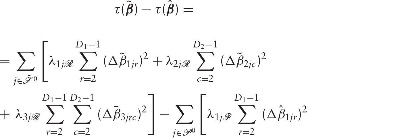
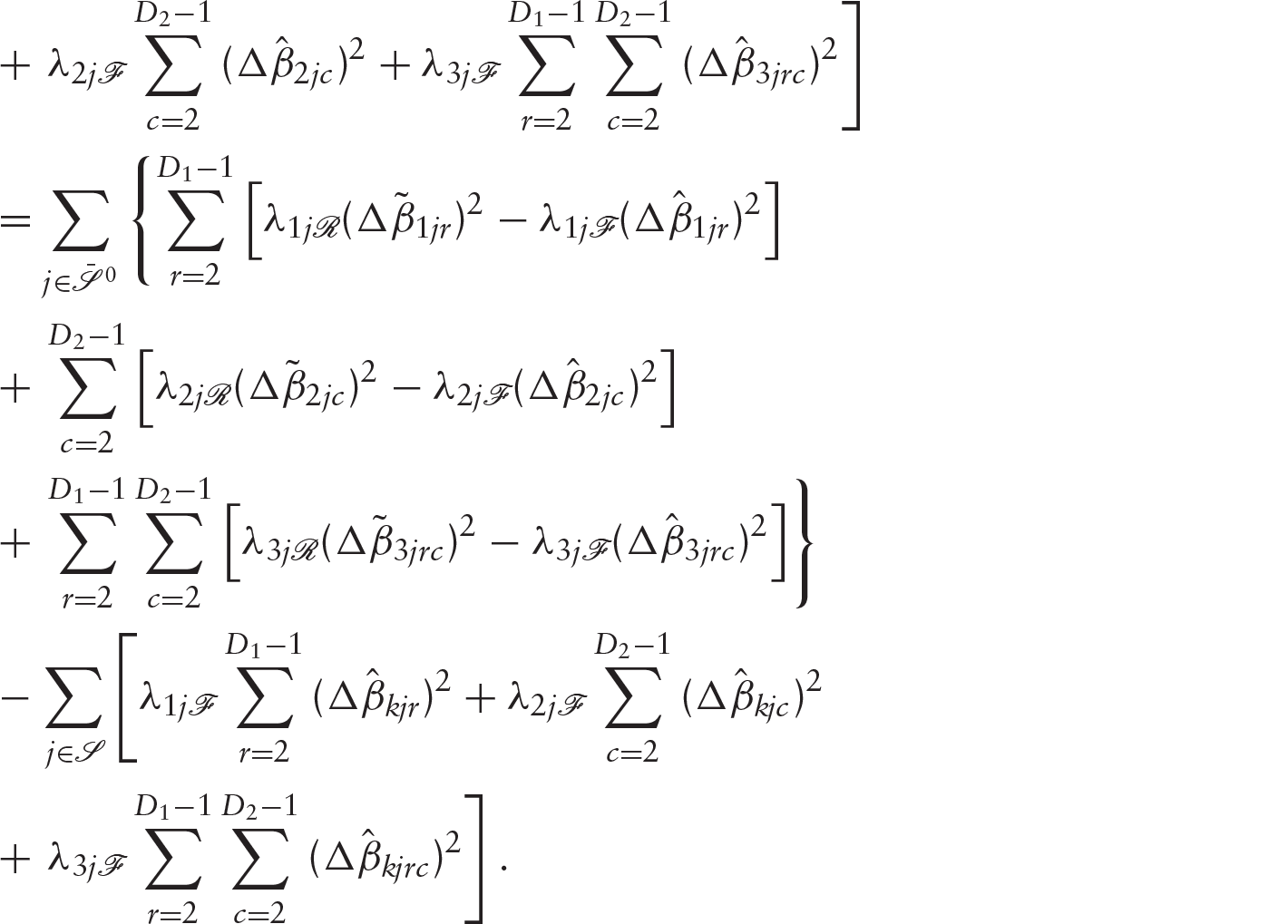
where ${\hat{π}}_{i}^{'} = ({\hat{π}}_{i 11}, \dots, {\hat{π}}_{{iD}_{1} D_{2}})^{'}$ is the estimated (by penalization) probability vector for the model under $H_{1}$ and ${\tilde{π}}_{i} = ({\tilde{π}}_{i 11}, \dots, {\tilde{π}}_{{iD}_{1} D_{2}})^{'}$ is the corresponding estimated (by penalization) probability vector for the reduced model. By supposing to use the penalty term ARC1 and by following Tutz and Scholz (2003), let $λ_{kj R} (λ_{kj F})$ denote the smoothing pameters for the reduced model (full model). Then, we have

\begin{matrix} = & \sum_{j \in {\bar{S}}^{0}} [λ_{1 j R} \sum_{r = 2}^{D_{1} - 1} (Δ {\tilde{β}}_{1 jr})^{2} + λ_{2 j R} \sum_{c = 2}^{D_{2} - 1} (Δ {\tilde{β}}_{2 jc})^{2} \\ + & λ_{3 j R} \sum_{r = 2}^{D_{1} - 1} \sum_{c = 2}^{D_{2} - 1} (Δ {\tilde{β}}_{3 jrc})^{2}] - \sum_{j \in P^{0}} [λ_{1 j F} \sum_{r = 2}^{D_{1} - 1} (Δ {\hat{β}}_{1 jr})^{2} \end{matrix}

\begin{matrix} + & λ_{2 j F} \sum_{c = 2}^{D_{2} - 1} (Δ {\hat{β}}_{2 jc})^{2} + λ_{3 j F} \sum_{r = 2}^{D_{1} - 1} \sum_{c = 2}^{D_{2} - 1} (Δ {\hat{β}}_{3 jrc})^{2}] \\ = & \sum_{j \in {\bar{S}}^{0}} \{\sum_{r = 2}^{D_{1} - 1} [λ_{1 j R} (Δ {\tilde{β}}_{1 jr})^{2} - λ_{1 j F} (Δ {\hat{β}}_{1 jr})^{2}] \\ + & \sum_{c = 2}^{D_{2} - 1} [λ_{2 j R} (Δ {\tilde{β}}_{2 jc})^{2} - λ_{2 j F} (Δ {\hat{β}}_{2 jc})^{2}] \\ + & \sum_{r = 2}^{D_{1} - 1} \sum_{c = 2}^{D_{2} - 1} [λ_{3 j R} (Δ {\tilde{β}}_{3 jrc})^{2} - λ_{3 j F} (Δ {\hat{β}}_{3 jrc})^{2}]\} \\ - & \sum_{j \in S} [λ_{1 j F} \sum_{r = 2}^{D_{1} - 1} (Δ {\hat{β}}_{kjr})^{2} + λ_{2 j F} \sum_{c = 2}^{D_{2} - 1} (Δ {\hat{β}}_{kjc})^{2} \\ + & λ_{3 j F} \sum_{r = 2}^{D_{1} - 1} \sum_{c = 2}^{D_{2} - 1} (Δ {\hat{β}}_{kjrc})^{2}] . \end{matrix}

If estimates are not penalized, that is, if for $k = 1, 2, 3$ , $λ_{k 1 R} = λ_{k 2 R} = \dots = λ_{k | {\bar{S}}^{0} | R} = λ_{k 0 F} = λ_{k 1 F} = \dots = λ_{k | P^{0} | F} = 0$ , one obtains $τ (\tilde{β}) - τ (\hat{β}) = 0$ , and the ${LR}_{P}$ statistic has the usual asymptotic $χ^{2}$ distribution. If $λ_{kj R} = λ_{kj F}$ is chosen for $j \in {\bar{S}}^{0}$ , $k = 1, 2, 3$ , then the first term is very small since ${\tilde{β}}_{kjr} \approx {\hat{β}}_{kjr}, {\tilde{β}}_{kjc} \approx {\hat{β}}_{kjc}$ and ${\tilde{β}}_{kjrc} \approx {\hat{β}}_{kjrc}$ for $r = 1, \dots, D_{1} - 1, c = 1, \dots, D_{2} - 1$ . Thus, the fundamental term concerns the variables for which $j \in S$ and, if estimates are penalized with a low smoothing value, converging to zero at an appropriate rate, the same asymptotic behaviour holds.

4 Simulation studies

The ${LR}_{P}$ sampling distributions discussed in the previous sections are shown here by simulation. We set two simulation schemes, called $sim 1$ and $sim 2$ , according to the two hypothesis systems in Sections 3.1 and 3.2, respectively. We generated $m = 1 000$ pseudo-samples from a multinomial distribution with probability matrix $Π (X β)$ and fitted reduced and unreduced models by penalizing the association ameter vector $β_{32}$ in $sim 1$ and the vector $β_{30}$ of association intercepts in $sim 2$ . The simulation setting is:

an equal number of levels in both responses and with values 3, 5 and 7;

sample sizes $n = 200$ , 500 and 1 000 when response levels are 3 or 5;

sample sizes $n = 1 000$ , 2 000 and 5 000 when response levels are 7;

$λ = 0$ , 0.2, 0.5, 1, 2, 5, 10, 20 and 50;

two binary covariates, $X_{1}$ and $X_{2}$ , both sampled from a $Ber (0.5)$ .

The set of $λ$ values used is typical of grid search algorithms. We preferred not to include further covariates because, especially for the cases with either 5 or 7 levels for both responses, the computational complexity of the estimation exponentially increases for each factor level added. The criterion used to set the order of magnitude of $n$ for the underlying table is to have, on average, 5 observations per cell. Accordingly, under a NUNPOM setting, for a simulation scheme with 3 levels per response and two binary variables, $n = 5 \times 3^{2} \times 2^{2} = 180$ (but it was rounded to 200). For the case with 5 levels $n = 5^{3} \times 2^{2} = 500$ , while $n = 5 \times 7^{2} \times 2^{2} = 980$ (rounded to 1 000) for the 7-level case.

4.1 Simulation scheme 1

In the first simulation scheme ( $sim 1$ ), we simulate the sampling distribution of the ${LR}_{P}$ statistic under the null hypothesis of Section 3.1. The pameters chosen to generate the simulation depend on the number of response levels. In ticular, these are specified as follows:

Simulation $sim 1$ : case $D_{1} = D_{2} = 3$

$β_{10} = (- 0.5, 0.5)^{'}, β_{11} = (0.2, 0.2)^{'}, β_{12} = (- 0.3, 0.3)^{'}$ ,

$β_{20} = (- 0.1, 0.6)^{'}, β_{21} = (0.3, 0.3)^{'}, β_{22} = (- 0.2, 0.4)^{'}$ ,

$β_{30} = (1.5, 2, 2.5, 3)^{'}, β_{31} = (- . 5, - . 5, - . 5, - . 5)^{'}, β_{32} = (0, 0, 0, 0)^{'}$ .

With this set of pameters, the model under the null hypothesis $β_{32 rc} = 0, r = 1, 2, c = 1, 2$ is a NUPPOM. The model under the alternative is a NUPPOM as well, but the ARC1 penalty term is applied to ameter vector $β_{32}$ .

Simulation $sim 1$ : case $D_{1} = D_{2} = 5$

$β_{10} = (- 0.8, 0.4, 1.2, 2.0)^{'}, β_{11 r} = 0.1, β_{12 r} = - 0.1, r = 1, \dots, 4$ ,

$β_{20} = (- 1.5, - 0.5, 0.3, 1.4)^{'}, β_{21 c} = 0.1, β_{22 c} = - 0.1, c = 1, \dots, 4$ ,

$β_{30} = (- 0.1, 0.0, 0.0, 0.4, 0.2, 0.2, 0.1, 0.3, 0.3, 0.2, 0.1, 0.1, 0.1, 0.2, 0.1, 0.4)^{'}, β_{31 rc} = - 0.5, β_{32 rc} = 0, r = 1, \dots, 4, c = 1, \dots, 4$ .

With this set of pameters (rounded for brevity), the model under the null hypothesis

β_{32 rc} = 0, r = 1, \dots, 4, c = 1, \dots, 4,

is a NUPOM. The model under the alternative is a NUPPOM, with the ARC1 penalty term applied to ameter vector

β_{32}

Simulation $sim 1$ : case $D_{1} = D_{2} = 7$

$β_{10} = (- 3.3, - 2.4, - 1.5, - 0.7, 1.1, 2.1)^{'}, β_{11 r} = - 0.1, β_{12 r} = 0.1, r = 1, \dots, 6$ ,

$β_{20} = (- 3.5, - 2.5, - 1.6, - 0.8, 0.9, 2.9)^{'}, β_{21 c} = - 0.1, β_{22 c} = 0.1, c = 1, \dots, 6$ ,

$β_{30} = (3.6, 2.9, 2.7, 2.3, 1.8, 2.1, 3.2, 2.9, 2.6, 2.2, 1.8, 2.0, 2.7, 2.4, 2.1, 1.7, 1.5, 1.3, 2.6, 2.1, 1.7, 1.5, 1.3, 1.2, 3.9, 2.2, 1.6, 1.2, 1.2, 1.0, 3.7, 2.3, 1.6, 1.2, 1.1, 1.2)^{'}, β_{31 rc} = 0.1, β_{32 rc} = 0, r = 1, \dots, 6, c = 1, \dots, 6$ .

With this set of pameters (rounded for brevity), the model under the null hypothesis

β_{32 rc} = 0, r = 1, \dots, 6, c = 1, \dots, 6,

is a NUPOM. The model under the alternative is a NUPPOM with the ARC1 penalty term applied to ameter vector

β_{32}

. The pameters chosen for the intercepts correspond to the observed global log odds and global odds ratios of the British male occupational study data of Section 6, with an adjustment of 0.0001 for sampling zeros in the original table.

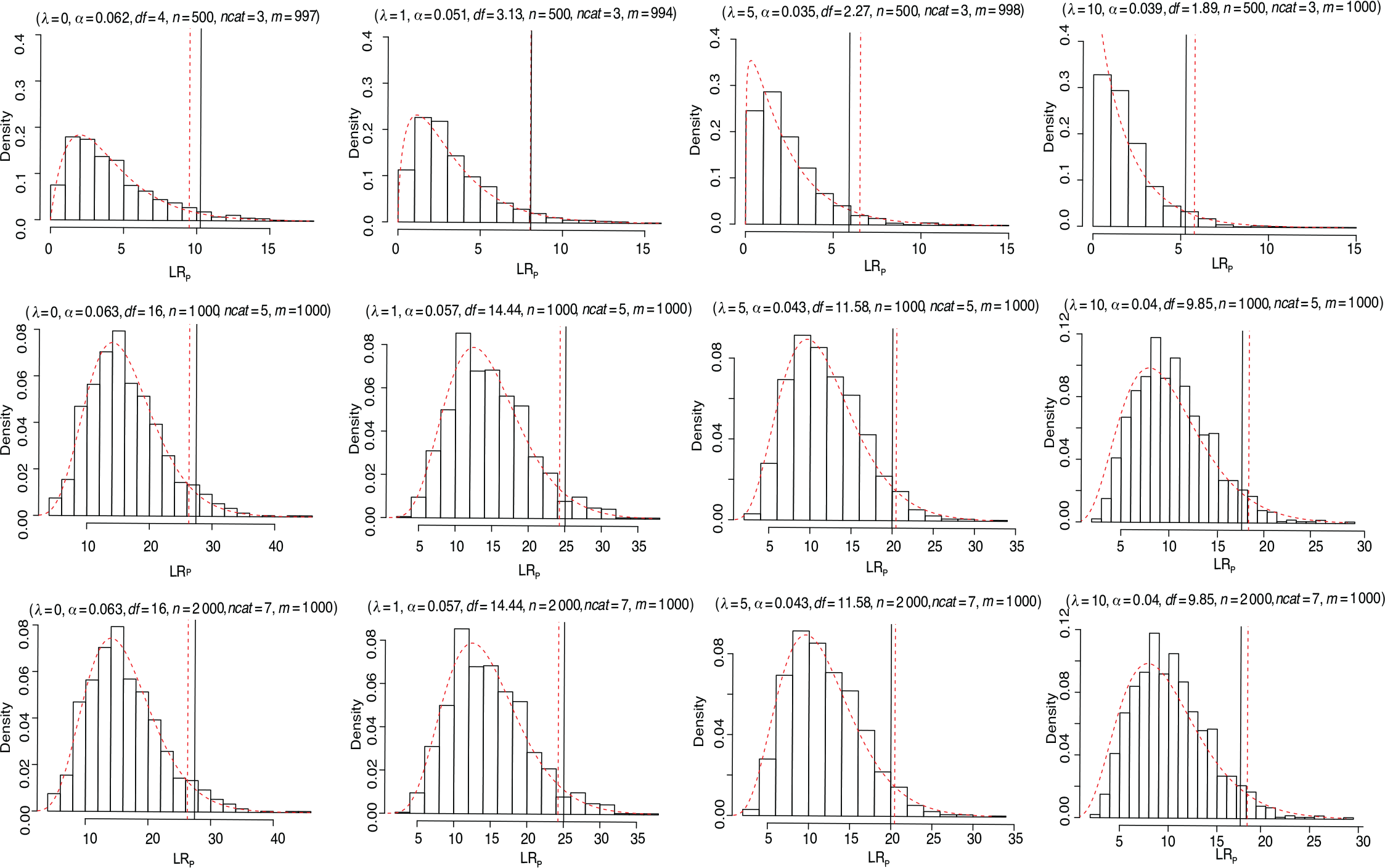
For the three cases outlined in scheme $sim 1$ , Figure 1 shows some selected histograms of the ${LR}_{P}$ simulated distribution with overimposed the theoretical $χ^{2}$ with $df$ degrees of freedom that depend on $λ$ . Sample sizes are $n = 200$ , 500 and 1 000 and correspond to the cases with 3, 5 and 7 levels ( $ncat$ ) per response. For brevity, only the histograms for a reduced set of $λ$ values are reported. The complete set of results for $sim 1$ is reported in Supplementary Material. Figure 2 shows the same scheme of Figure 1, but with sample sizes $n$ increased to 500, 1 000 and 2 000, respectively, for $ncat = 3$ , 5 and 7.

Figure 1:

Histograms of the simulated distribution of ${LR}_{P}$ from the scheme $sim 1$ for varying $λ$ (left to right) and number of response levels $ncat$ (up to down). Sample sizes are $n = 200$ , 500 and 1 000 and vary according to $ncat$ , while $m$ indicates the number of valid pseudo-samples. The overimposed dashed curve is a $χ^{2}$ with $df$ degrees of freedom. $α$ is the empirical significance level. The vertical dashed and continuous lines are in correspondence of the $95 th$ percentile of the theoretical and the empirical distribution, respectively

Figure 2:

Histograms of the simulated distribution of ${LR}_{P}$ from the scheme $sim 1$ for varying $λ$ (left to right) and number of response levels $ncat$ (up to down). Sample sizes are $n = 500$ , 1 000 and 2 000 and vary according to $ncat$ , while $m$ indicates the number of valid pseudo-samples. The overimposed dashed curve is a $χ^{2}$ with $df$ degrees of freedom. $α$ is the empirical significance level. The vertical dashed and continuous lines are in correspondence of the $95 th$ percentile of the theoretical and the empirical distribution, respectively

Although the number $m$ of pseudo-samples for this simulation was fixed to 1 000, their effective number is reduced because it was based on those models that successfully converged.

Overall, the complete set of results for this simulation scheme (reported in the Supplementary Materials) shows a good approximation for larger $n$ and smaller $λ$ .

4.2 Simulation scheme 2

In the second simulation scheme ( $sim 2$ ), the sampling distribution of the ${LR}_{P}$ statistic is simulated under the null hypothesis in Section 3.2. In all scenarios, the reduced model is a NUPOM and the null hypothesis fixes $β_{32 rc}$ to a unique value. The model under the alternative is a NUPPOM as $β_{32 rc}$ is unconstrained. In both models, ARC1 is applied to their association intercepts $β_{30}$ using the same value of the penalty ameter $λ$ . The pameters chosen to generate the simulation depend on the number of response levels. In ticular, these are specified as follows:

Simulation $sim 2$ , case $D_{1} = D_{2} = 3$

$β_{10} = (- 0.5, 0.5)^{'}, β_{11} = (0.2, 0.2)^{'}, β_{12} = (- 0.3, 0.3)^{'}$ ,

$β_{20} = (- 0.1, 0.6)^{'}, β_{21} = (0.3, 0.3)^{'}, β_{22} = (- 0.2, 0.4)^{'}$ ,

$β_{30} = (1.5, 2, 2.5, 3)^{'}, β_{31} = (- . 2, - . 2, - . 2, - . 2)^{'}, β_{32} = (0.5, 0.5, 0.5, 0.5)^{'}$ .

With this set of pameters the null hypothesis is $β_{32 rc} = 0.5, r = 1, 2, c = 1, 2$ .

Simulation $sim 2$ , case $D_{1} = D_{2} = 5$

$β_{10} = (- 0.8, 0.4, 1.2, 2.0)^{'}, β_{11 r} = 0.1, β_{12 r} = - 0.1, r = 1, \dots, 6$ ,

$β_{20} = (- 1.5, - 0.5, 0.3, 1.4)^{'}, β_{21 c} = 0.1, β_{22 c} = - 0.1, c = 1, \dots, 4$ ,

$β_{30} = (- 0.1, 0.0, 0.0, 0.4, 0.2, 0.2, 0.1, 0.3, 0.3, 0.2, 0.1, 0.1, 0.1, 0.2, 0.1, 0.4)^{'}, β_{31 rc} = 0.2, β_{32 rc} = 0.4, r = 1, \dots, 4, c = 1, \dots, 4$ .

With this set of pameters (rounded for brevity to the first decimal point), the null hypothesis is $β_{32 rc} = 0.4, r = 1, \dots, 4, c = 1, \dots, 4$ .

Simulation $sim 2$ , case $D_{1} = D_{2} = 7$

$β_{10} = (- 3.1 - 2.3 - 1.4 - 0.71.12.1)^{'}, β_{11 r} = - 0.1, β_{12 r} = 0.1, r = 1, \dots, 6$ ,

$β_{20} = (- 3.3, - 2.4, - 1.5, - 0.8, 0.9, 2.0)^{'}, β_{21 c} = - 0.1, β_{22 c} = 0.1, c = 1, \dots, 6$ ,

$β_{30} = (3.2, 2.6, 2.5, 2.0, 1.4, 1.4, 2.8, 2.6, 2.4, 2.0, 1.4, 1.4, 2.4, 2.2, 1.9, 1.6, 1.3, 1.1, 2.2, 1.9, 1.6, 1.4, 1.2, 1.1, 1.8, 1.5, 1.3, 1.1, 1.1, 0.9, 1.5, 1.4, 1.2, 1.0, 1.0, 1.1)^{'}, β_{31 rc} = - 0.1, β_{32} = 0.4, r = 1, \dots, 6, c = 1, \dots, 6$ .

With this set of pameters (rounded), the null hypothesis is $β_{32 rc} = 0.4, r = 1, \dots, 6, c = 1, \dots, 6$ . The pameters chosen for the intercepts correspond to the observed global log odds and global odds ratios of the British male occupational study data of Section 6, with an adjustment of 0.001 for sampling zeros in the original table.

For the simulation scheme 2, Figure 3 shows some selected histograms of the ${LR}_{P}$ simulated distribution with overimposed the theoretical $χ^{2}$ with 3, 15 and 35 degrees of freedom, and for $ncat = 3$ , 5 and 7 levels, respectively. Sample sizes are $n = 200$ , 500 and 1 000 and correspond to $ncat = 3$ , 5 and 7, as well. The complete set of results for $sim 2$ is reported in Supplementary Material.

Figure 3:

Histograms of the simulated distribution of ${LR}_{P}$ from the scheme $sim 2$ for varying $λ$ (left to right) and number of response levels $ncat$ (up to down). Sample sizes are $n = 200$ , 500 and 1 000 and vary according to $ncat$ , while $m$ indicates the number of valid pseudo-samples. The overimposed dashed curve is a $χ^{2}$ with $df$ degrees of freedom. $α$ is the empirical significance level. The vertical dashed and continuous lines are in correspondence of the $95 th$ percentile of the theoretical and the empirical distribution, respectively

Figure 4 shows the same scheme of Figure 3, but with sample sizes $n$ increased to 500, 1 000 and 2 000, respectively, for $ncat = 3, 5$ and 7.

Figure 4:

Histograms of the simulated distribution of ${LR}_{P}$ from the scheme $sim 2$ for varying $λ$ (left to right) and number of response levels $ncat$ (up to down). Sample sizes are $n = 500$ , 1 000 and 2 000 and vary according to $ncat$ , while $m$ indicates the number of valid pseudo-samples. The overimposed dashed curve is a $χ^{2}$ with $df$ degrees of freedom. $α$ is the empirical significance level. The vertical dashed and continuous lines are in correspondence of the $95 th$ percentile of the theoretical and the empirical distribution, respectively

Overall, the histograms for $sim 2$ shows a good approximation of the theoretical $χ^{2}$ to the ${LR}_{P}$ sampling distribution for larger $n$ and smaller $λ$ . On the contrary, the approximation is very poor, especially for $λ > 10$ (see also Supplementary Material).

5 Evaluating the performance of penalized estimates

In order to evaluate the potential of smoothed estimates, a simulation study for the case with three response levels and one continuous covariates is carried out. Three sample sizes are considered $n = 200$ , 500 and 1 000, whereas the number of samples is taken to be $m = 1 000$ . The simulations are generated from a $NUNPOM$ with the following pameters:

$β_{10} = (- 0.6, 0.6)^{'}, β_{11} = (0.3, - 0.3)^{'}$ ,

$β_{20} = (- 0.6, 0.6)^{'}, β_{21} = (- 0.3, 0.3)^{'}$ ,

$β_{30} = (2.6, 2.4, 2.0, 1.7)^{'}, β_{31} = (- 0.4, 0.2, - 0.5, 0.5)^{'}$ .

The values $x_{i}, i = 1, \dots, n$ of the covariate were drawn from a $U (- 1, 1)$ . Thus, given the model formula (2.6) and the inversion method (2.4), we found the $n \times (D_{1} D_{2})$ probability matrix $Π$ , in which each row $π_{i}^{'}$ represents the probability vector for the $i$ th observation. Then, the responses were drawn from a multinomial distribution with probability vector $π_{i}^{'}$ . The $UPOM$ was comed to the $NUNPOM$ , for which ARC1 has been used in combination with (2.16). Penalization pameters for ARC1, that is, $λ_{1}, λ_{2}$ and $λ_{3}$ were chosen equal to a single value $λ$ , varying in the set ${0, 1, 10, 100, \dots}$ . The results of the simulation were evaluated by the number of Fisher scoring successes, by the AIC (defined in Appendix A), by the loss functions.

Mean squared error loss:

MSEL = \frac{1}{n} \sum_{i = 1}^{n} \sum_{r = 1}^{D_{1} D_{2}} (π_{ir} - {\hat{π}}_{ir})^{2},

(5.1)

Mean relative squared error loss:

MRSEL = \frac{1}{n} \sum_{i = 1}^{n} \sum_{r = 1}^{D_{1} D_{2}} \frac{(π_{ir} - {\hat{π}}_{ir})^{2}}{π_{ir}},

(5.2)

Mean entropy or Kullback–Leibler loss:

MEL = \frac{1}{n} \sum_{i = 1}^{n} \sum_{r = 1}^{D_{1} D_{2}} π_{ir} \log (\frac{π_{ir}}{{\hat{π}}_{ir}}),

(5.3)

and by the overall Relative Bias:

RBIAS = \frac{1}{FSS} \sum_{f = 1}^{FSS} \sum_{k = 1}^{3} \sum_{q = 1}^{Q_{k}} \frac{| {\hat{β}}_{fkq} - β_{fkq} |}{β_{fkq}},

(5.4)

where $FSS$ is the number of Fisher scoring successes. ${\hat{β}}_{fkq}$ and $β_{fkq}$ represent the $q$ th estimated ameter and the $q$ th true ameter, respectively, in the $k$ th model equation of the $f th$ simulation. In our example, $Q_{1} = Q_{2} = 4$ , while $Q_{3} = 8$ .

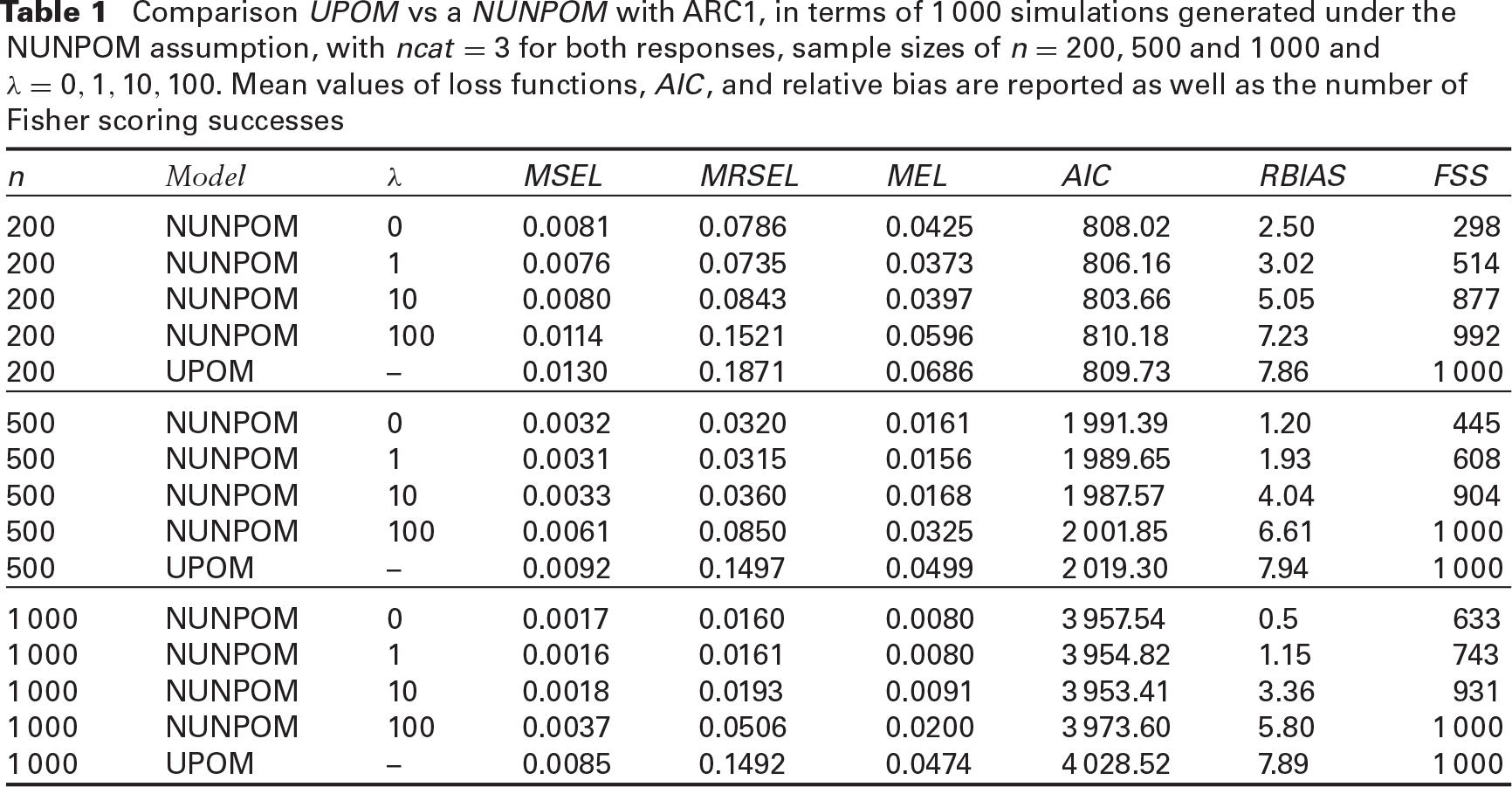
Before setting $λ$ to some value greater than zero, some attempts to estimate the model were made by reducing the step length $l_{step}$ of the iterative algorithm (see Appendix A), and in some case the $NUNPOM$ was fitted. Actually, this step length reduction is automatically performed with the ‘pblm’ R package provided along with this article. The $UPOM$ was fitted in all simulations. The results are reported in Table 1, while Table 2 reports the mean estimated $β$ .

Table 1:

Comison $UPOM$ vs a $NUNPOM$ with ARC1, in terms of 1 000 simulations generated under the NUNPOM assumption, with $ncat = 3$ for both responses, sample sizes of $n = 200$ , 500 and 1 000 and $λ = 0, 1, 10, 100$ . Mean values of loss functions, $AIC$ , and relative bias are reported as well as the number of Fisher scoring successes

$n$	Model	$λ$	MSEL	MRSEL	MEL	AIC	RBIAS	FSS
200	NUNPOM	0	0.0081	0.0786	0.0425	808.02	2.50	298
200	NUNPOM	1	0.0076	0.0735	0.0373	806.16	3.02	514
200	NUNPOM	10	0.0080	0.0843	0.0397	803.66	5.05	877
200	NUNPOM	100	0.0114	0.1521	0.0596	810.18	7.23	992
200	UPOM	–	0.0130	0.1871	0.0686	809.73	7.86	1 000
500	NUNPOM	0	0.0032	0.0320	0.0161	1 991.39	1.20	445
500	NUNPOM	1	0.0031	0.0315	0.0156	1 989.65	1.93	608
500	NUNPOM	10	0.0033	0.0360	0.0168	1 987.57	4.04	904
500	NUNPOM	100	0.0061	0.0850	0.0325	2 001.85	6.61	1 000
500	UPOM	–	0.0092	0.1497	0.0499	2 019.30	7.94	1 000
1 000	NUNPOM	0	0.0017	0.0160	0.0080	3 957.54	0.5	633
1 000	NUNPOM	1	0.0016	0.0161	0.0080	3 954.82	1.15	743
1 000	NUNPOM	10	0.0018	0.0193	0.0091	3 953.41	3.36	931
1 000	NUNPOM	100	0.0037	0.0506	0.0200	3 973.60	5.80	1 000
1 000	UPOM	–	0.0085	0.1492	0.0474	4 028.52	7.89	1 000

In the simulation with $n = 200$ and $λ = 0$ , Fisher scoring failed in 702 out of 1 000 simulations, while almost all models were successfully estimated when $λ = 100$ . Observe that all the mean loss functions and $AIC$ for the $NUNPOM$ are smaller than the $UPOM$ ones, as it should be. The $NUNPOM$ without penalization (i.e., $λ = 0$ ) has the smallest loss functions values, but also the greatest $AIC$ value among the $NUNPOMs$ .

As expected (Table 2), especially for the NUNPOM pameters involved in the penalization, the larger $λ$ values the larger the ameter bias. However, overall, the bias appears to be smaller than the UPOM one. Further, the bias decreases as $n$ increases.

6 Applications to real datasets

6.1 The British male occupational status dataset

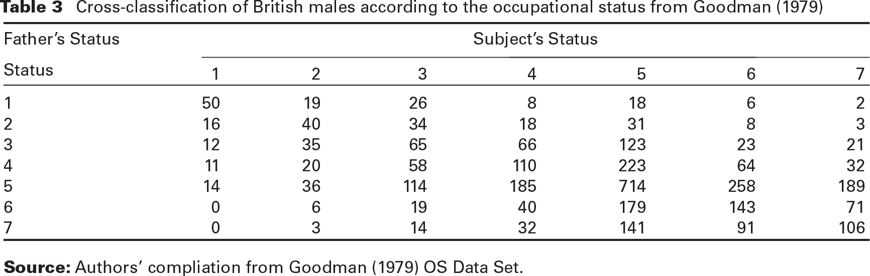
Consider the data on occupational status (OS) of a sample of British males from Goodman (1979), where fathers and their sons were cross-classified according to the OS using seven ordered categories. The data are reported in Table 3.

Several authors have re-analysed such data. For example, Lapp et al. (1998) come the Goodman RC and Dale models in terms of goodness of fit. We further re-analyse the data by fitting the BOLM with ARC2. The aim of the application is to show the advantages of our proposal when comed to the existing alternatives.

The saturated model for the joint distribution involves 48 ameters: 6 global logits for each marginal and 36 log-GORs. Since the interest is in modelling the association structure, the focus is on the 36 log-GORs only. Figure 5 shows the AIC for the NUPOM for varying smoothing ameter and different orders of penalization.

Table 2:

Comison $UPOM$ vs $NUNPOM$ with ARC1 in terms of mean pameters of 1 000 simulations, of sizes $n = 200$ , 500 and 1 000, generated under the NUNPOM assumption with $ncat = 3$ for both responses

$n$	Model	$λ$	$β_{101}$	$β_{102}$	$β_{111}$	$β_{112}$	$β_{201}$	$β_{202}$	$β_{211}$	$β_{212}$	$β_{301}$	$β_{302}$	$β_{303}$	$β_{304}$	$β_{305}$	$β_{312}$	$β_{313}$	$β_{314}$
200	TRUE MODEL	0	$-$ 0.60	0.60	0.30	$-$ 0.30	$-$ 0.60	0.60	$-$ 0.30	0.30	2.60	2.40	2.00	1.70	$-$ 0.40	0.20	$-$ 0.50	0.50
200	NUNPOM	0	$-$ 0.61	0.60	0.28	$-$ 0.27	$-$ 0.62	0.60	$-$ 0.27	0.29	2.68	2.61	2.17	1.73	$-$ 0.40	$-$ 0.08	$-$ 0.27	0.48
200	NUNPOM	1	$-$ 0.60	0.61	0.28	$-$ 0.25	$-$ 0.61	0.61	$-$ 0.28	0.27	2.69	2.51	2.12	1.69	$-$ 0.25	$-$ 0.03	$-$ 0.15	0.39
200	NUNPOM	10	$-$ 0.59	0.59	0.21	$-$ 0.17	$-$ 0.59	0.59	$-$ 0.26	0.14	2.72	2.46	2.14	1.69	0.03	0.07	0.07	0.22
200	NUNPOM	100	$-$ 0.59	0.59	0.10	0.01	$-$ 0.60	0.60	$-$ 0.16	$-$ 0.07	2.69	2.50	2.12	1.62	0.14	0.14	0.14	0.16
200	UPOM	–	$-$ 0.59	0.59	0.06	$-$ 0.61	0.61	$-$ 0.13	2.65	2.50	2.11	1.59	0.15	$-$ 0.59	0.59	0.06	$-$ 0.61	0.61
500	NUNPOM	0	$-$ 0.61	0.61	0.29	$-$ 0.29	$-$ 0.60	0.61	$-$ 0.29	0.28	2.63	2.48	2.05	1.70	$-$ 0.39	0.07	$-$ 0.39	0.52
500	NUNPOM	1	$-$ 0.61	0.60	0.29	$-$ 0.28	$-$ 0.60	0.60	$-$ 0.31	0.28	2.64	2.44	2.04	1.69	$-$ 0.34	0.01	$-$ 0.27	0.46
500	NUNPOM	10	$-$ 0.60	0.60	0.26	$-$ 0.24	$-$ 0.59	0.59	$-$ 0.31	0.21	2.70	2.38	2.07	1.65	$-$ 0.10	$-$ 0.01	$-$ 0.02	0.27
500	NUNPOM	100	$-$ 0.60	0.60	0.14	$-$ 0.05	$-$ 0.58	0.58	$-$ 0.21	$-$ 0.02	2.69	2.43	2.08	1.60	0.09	0.10	0.10	0.14
500	UPOM	–	$-$ 0.61	0.61	0.07	$-$ 0.59	0.58	$-$ 0.15	2.63	2.45	2.07	1.56	0.11	$-$ 0.61	0.61	0.07	$-$ 0.59	0.58
1 000	NUNPOM	0	$-$ 0.60	0.60	0.29	$-$ 0.30	$-$ 0.60	0.61	$-$ 0.30	0.29	2.60	2.43	2.01	1.69	$-$ 0.40	0.13	$-$ 0.48	0.50
1 000	NUNPOM	1	$-$ 0.60	0.60	0.30	$-$ 0.29	$-$ 0.60	0.60	$-$ 0.31	0.28	2.62	2.41	2.01	1.69	$-$ 0.36	0.08	$-$ 0.39	0.46
1 000	NUNPOM	10	$-$ 0.60	0.59	0.28	$-$ 0.27	$-$ 0.60	0.59	$-$ 0.32	0.24	2.68	2.37	2.03	1.66	$-$ 0.19	$-$ 0.04	$-$ 0.13	0.31
1 000	NUNPOM	100	$-$ 0.59	0.59	0.18	$-$ 0.12	$-$ 0.58	0.58	$-$ 0.25	0.06	2.70	2.40	2.05	1.63	0.05	0.07	0.06	0.15
1 000	UPOM	–	$-$ 0.60	0.60	0.07	$-$ 0.59	0.59	$-$ 0.15	2.60	2.44	2.04	1.56	0.10	$-$ 0.60	0.60	0.07	$-$ 0.59	0.59

Table 3:

Cross-classification of British males according to the occupational status from Goodman (1979)

Father's Status	Subject's Status
Status	1	2	3	4	5	6	7
1	50	19	26	8	18	6	2
2	16	40	34	18	31	8	3
3	12	35	65	66	123	23	21
4	11	20	58	110	223	64	32
5	14	36	114	185	714	258	189
6	0	6	19	40	179	143	71
7	0	3	14	32	141	91	106

Source: Authors’ compliation from Goodman (1979) OS Data Set.

Figure 5:

OS dataset: The left plot shows the AIC for varying smoothing ameter $λ$ (in log scale) for a NUPOM using the penalty term ARC2 on the association intercepts. Different orders $s$ of penalization are used assuming $s_{3} = s_{4} = s$ . For $\log λ \to + \infty$ , $s = 1$ (dotted line) the model AIC will tend to the UPOM level; $s = 2$ (dashed line), $s = 3$ (dotted-dashed line) and $s = 4$ (continuous line) correspond to AIC of models tending to a polynomial from first to third degree, respectively. The plot on the right shows the detail of the most critical interval, where the AIC is minimized for $\log λ = 4$ and $s = 3$

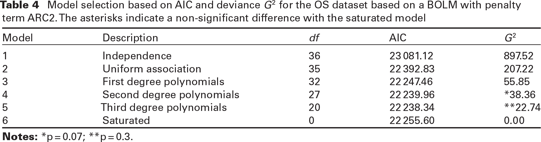
Due to the symmetry of the association structure, the penalization orders of the difference operator $s_{3}$ and $s_{4}$ are assumed to be equal and indicated by $s$ . The AIC for the model with $s = 1$ tends to the UPOM AIC level for high values of log $λ$ . This model is clearly inadequate as the models specified by higher $s$ provide smaller AIC whatever $\log λ$ . The minimum value of AIC is $22 236.65$ , corresponding to $\log (λ) = 4$ and $s = 3$ . This represents a model with an association structure which tends to a smooth surface defined by row and column interactions of second degree polynomials. On the grounds of $AIC$ only, one could choose this model. However, for high values of $λ$ , the models with $s = 3 (AIC = 22 239.96)$ and $s = 4 (AIC = 22 238.34)$ provide good fits as well, with a slight evidence in favour of the latter model, corresponding to a polynomial surface of third degree. The AIC differences of such models, with respect to the minimum AIC, are respectively 3.31 and 1.69, which are quite small (Burnham and Anderson, 2000, p. 48). When it is possible, as in this case, it is preferable to choose a model providing integer and equally spaced scores, on the grounds of greater interpretability and for the possibility to use classical test statistics whose asymptotic null distributions are well known. Therefore, we report in Table 4 the results (in terms of $AIC$ and deviance $G^{2}$ ) for the four polynomial models evaluated at the largest value of $\log (λ) = 15$ , along with the independence and saturated models.

Table 4:

Model selection based on AIC and deviance $G^{2}$ for the OS dataset based on a BOLM with penalty term ARC2. The asterisks indicate a non-significant difference with the saturated model

Model	Description	$df$	AIC	$G^{2}$
1	Independence	36	23 081.12	897.52
2	Uniform association	35	22 392.83	207.22
3	First degree polynomials	32	22 247.46	55.85
4	Second degree polynomials	27	22 239.96	*38.36
5	Third degree polynomials	20	22 238.34	**22.74
6	Saturated	0	22 255.60	0.00

note [*p = 0.07; **p = 0.3.]

Model 1 has been fitted by using the ridge-type penalty term, such that the estimated global log-odds ratios tend to zero for high values of the smoothing ameter. Model 4 provides the most simonious but yet acceptable fit, with only 9 estimated pameters and $p$ -value = 0.07. Model 5 estimates only 16 ameters, providing a comable fit ( $G^{2} = 22.74$ ), with a not significant difference with the saturated model ( $p$ -value = 0.3). This means the ordinal association structure of OS can be well fitted by a polynomial of second or third degree. Notice that Models 4 and 5 are more simonious than the best model found in Lapp et al.’s analysis, that is, the Dale model, including row effects, column effects, and interactions, while maintaining a comable fit in terms of $G^{2}$ . The observed structure of global log-odds ratios and the selected polynomial models are graphically showed in Figure 6.

Figure 6:

Association structures for the OS dataset. In lexicographical order: observed log-GORs (top-left); log-GORs fitted by the interaction of polynomials of second degree with non-integer scores (top-right); log-GORs fitted by the interaction of polynomials of second (bottom-left) and third (bottom-right) degree with integer scores

As we can see, the ordinal association structure is always positive, but it decreases as both the social statuses increase. Observe that the second degree polynomials using integer and non-integer scores show very slight differences. Finally, notice that also Lapp et al. hypothesized the possibility to fit a ‘symmetric second degree polynomial’ model.

6.2 The liver disease patients dataset

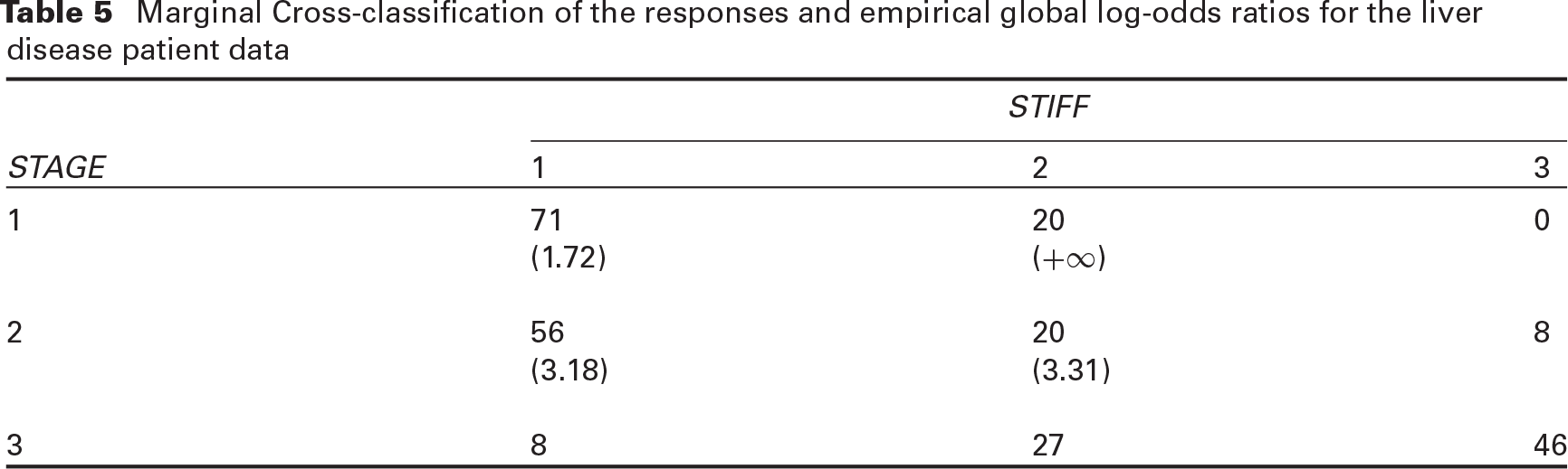
The dataset consists of 256 patients with a liver disease progression. The two outcomes, both measured on the same day, are the liver biopsy (named STAGE), considered the natural gold standard, and a categorized version of transient elastography (STIFF) according to cut-offs suggested by Castera et al. (2005), to measure liver stiffness. Both responses have three ordered categories, STIFF with levels 1,2 and 3, which correspond to stiffness classes $[0, 7.1)$ , $[7.1, 12.5)$ and $[12.5, \infty)$ , respectively; as for STAGE, the initial five categories F0–F4 have been collapsed as follows: 1, corresponding to the biopsy stage $< F 2$ , 2 ( $= {F 2, F 3}$ ) and 3 ( $= F 4$ ). Aim of the study is to evaluate the concordance between the outcomes in order to find profiles of ‘discordant’ patients. This is done using the bivariate logistic model, by employing the log global odds as marginal pameters and the log global odds ratio as association measure. For these data, a first analysis with dichotomized responses was made by Calvaruso et al. (2010). Table 5 shows the cross-classification of the responses, ignoring covariates.

Table 5:

Marginal Cross-classification of the responses and empirical global log-odds ratios for the liver disease patient data

	STIFF
STAGE	1	2	3
1	71	20	0
	(1.72)	( $+ \infty$ )

2	56	20	8
	(3.18)	(3.31)

3	8	27	46

From a first look at Table 5, it is possible to notice a positive association between the responses, even if there are many discordant patients, mainly the 56 in $STAGE = 2, STIFF = 1$ . Among the covariates, the patient's gender (SEX), age (AGE), alanine aminotransferase (ALT) measured in $U / L$ and platelet (PLT) levels measured in $10^{3}$ mmc, are considered. For modelling purposes, the covariates were centred with respect to their means and, after a backward selection, we considered the following sets of variables:

P_{1}^{0} = {{Intercept}_{\bar{123}}, {SEX}_{123}, {AGE}_{123}, {ALT}_{123}, {PLT}_{1 \bar{2} 3}},

P_{2}^{0} = {{Intercept}_{\bar{123}}, {SEX}_{123}, {AGE}_{123}, {ALT}_{123}, {PLT}_{123}},

P_{3}^{0} = {{Intercept}_{\bar{12} 3}, {SEX}_{123}, {AGE}_{123}, {ALT}_{123}, {PLT}_{1 \bar{2} 3}},

P_{4}^{0} = {{Intercept}_{\bar{12} 3}, {SEX}_{123}, {AGE}_{123}, {ALT}_{123}, {PLT}_{123}},

P_{5}^{0} = {{Intercept}_{\bar{123}}, {AGE}_{123}, {ALT}_{123}, {PLT}_{1 \bar{2} 3}},

P_{6}^{0} = {{Intercept}_{\bar{123}}, {AGE}_{123}, {ALT}_{123}, {PLT}_{1 \bar{2}}},

P_{7}^{0} = {{Intercept}_{\bar{123}}, {AGE}_{12}, {ALT}_{123}, {PLT}_{1 \bar{2}}},

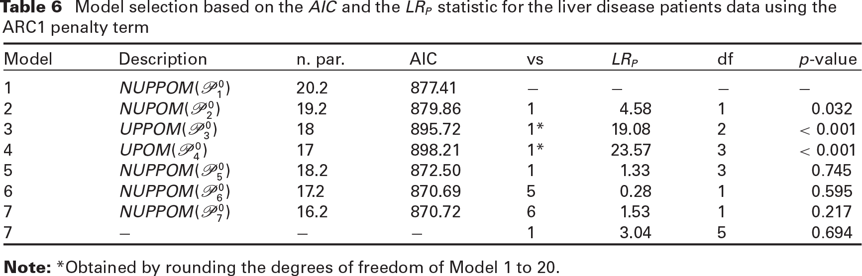
where Intercept₁₂₃ indicates that the marginal and association intercepts are category dependent, whereas Intercept₁₂₃ indicates that the intercepts for the association are category independent. To indicate that variable $AGE$ is included both in marginal and association predictors, we use ${AGE}_{123}$ , whereas ${AGE}_{12}$ indicates that such variable is included only in the marginal predictors. Computational problems had arisen when we tried to estimate non-uniform association models. Such problems were overcome by regularizing the ameter space of the association intercepts. In ticular, the ARC1 penalty term was employed, with smoothing ameter $λ_{3} = 0.5$ , which is the value that minimizes the AIC. This value was found through the two-step procedure described in Section 2.1.1. By considering the results from the simulation in Section 3, we decided to use a $χ^{2}$ distribution to approximate the ${LR}_{P}$ asymptotic distribution. The results of model selection are reported in Table 6.

Table 6:

Model selection based on the $AIC$ and the ${LR}_{P}$ statistic for the liver disease patients data using the ARC1 penalty term

Model	Description	n. .	AIC	vs	${LR}_{P}$	df	$p$ -value
1	$NUPPOM (P_{1}^{0})$	20.2	877.41	$-$	$-$	$-$	$-$
2	$NUPOM (P_{2}^{0})$	19.2	879.86	1	4.58	1	$0.032$
3	$UPPOM (P_{3}^{0})$	18	895.72	1*	19.08	2	$< 0.001$
4	$UPOM (P_{4}^{0})$	17	898.21	1*	23.57	3	$< 0.001$
5	$NUPPOM (P_{5}^{0})$	18.2	872.50	1	1.33	3	$0.745$
6	$NUPPOM (P_{6}^{0})$	17.2	870.69	5	0.28	1	$0.595$
7	$NUPPOM (P_{7}^{0})$	16.2	870.72	6	1.53	1	$0.217$
7	$-$	$-$	$-$	1	3.04	5	$0.694$

note [*Obtained by rounding the degrees of freedom of Model 1 to 20.]

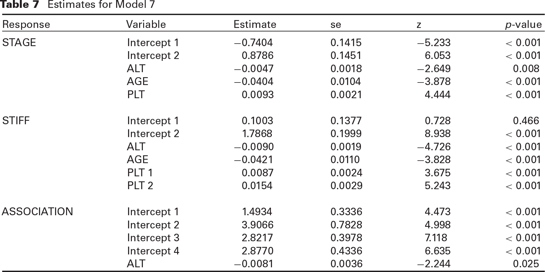
For each model that we have selected, the table reports its description, the number of estimated pameters and the AIC. The next columns refer to the comisons between nested models, specified by the column headed ‘vs’. The last three columns report the results of such comison in terms of penalized log-likelihood ratio statistic, along with degrees of freedom and $p$ -values. Before proceeding to variable selection, the hypothesis $UPOM$ , versus alternatives $UPPOM$ , $NUPOM$ and $NUPPOM$ were checked for all variables. The table reports the comisons for Models 1–4. Model 1 is the most complex model we have considered, a $NUPPOM$ defined on set $P_{1}^{0}$ . This model assumes that the effect of variable $PLT$ on $STIFF$ depends on the categories of $STIFF$ . Models 2–4 represent hypotheses of uniform association and/or (tially) proportional odds, and these models are comed to Model 1, for which none of these hypotheses holds. Although the ${LR}_{P}$ test for model comison is approximated, some results seem to be clear. For example, because the difference between Models 1 and 3 (or 4) is highly significant, the hypothesis of $UPPOM$ (or $UPOM$ ) does not hold. Models 5–7 concern a backward model selection starting from Model 1. The last row reports the comison between Models 7 and 1, for which the difference between the starting model and the final model is not significant ( $p$ -value $=$ 0.711). In Model 7, variable $ALT$ is the only one which has significant (global) effect for the association model. By AIC, the model with the best trade-off between goodness of fit and simony is still Model 7. Figure 7 shows the comison between the simulated distribution of ${LR}_{P}$ for the comison between the models in Table 6.

Figure 7:

Simulated distribution of ${LR}_{P}$ for the comison between the models in Table 6. The overimposed dashed curve is a $χ^{2}$ distribution. The vertical lines are in correspondence of the 95th percentile of the theoretical and the empirical distribution, respectively

Models 3 and 4 are not involved in this simulation for the reason explained earlier. $α$ is the real significance level obtained using the 95th percentile of the $χ^{2}$ distribution (dashed curve) with respect to the empirical one, while m* indicates the number of valid pseudo-samples from the initial m $=$ 1 500. Vertical dashed and continuous lines are in correspondence of the 95th percentile of the theoretical and the empirical distribution, respectively.

Overall, there is a good correspondence when the $χ^{2}$ distribution is used to approximate the simulated distribution, except for the comison between Models 1 and 2. For this comison, the real significance level, when using the 95th percentile of the $χ_{1}^{2}$ , is $α = 0.03$ , resulting to be more conservative. Estimates for the final Model 7 are reported in Table 7. Variables $ALT$ , $AGE$ and $PLT$ are significant in both marginal outcomes. In ticular, the platelet level has a category-dependent effect for $STIFF$ , which is higher for the log global odds 1–2 than 3. In ticular, a patient at older age, higher $ALT$ and lower $PLT$ values is more at risk of having a greater liver stiffness than a patient with mean values. In addition, the $ALT$ effect for $STIFF$ is about twice as strong as for biopsy stage. The effect of $ALT$ in the association is significant, and considering the intercepts values as well, higher $ALT$ values imply a global reduction of the association, especially for individuals in class $STIFF < 7.1$ and $STAGE = 1$ .

Table 7:

Estimates for Model 7

Response	Variable	Estimate	se	z	$p$ -value
STAGE	Intercept 1	$-$ 0.7404	0.1415	$-$ 5.233	$< 0.001$
	Intercept 2	0.8786	0.1451	6.053	$< 0.001$
	ALT	$-$ 0.0047	0.0018	$-$ 2.649	0.008
	AGE	$-$ 0.0404	0.0104	$-$ 3.878	$< 0.001$
	PLT	0.0093	0.0021	4.444	$< 0.001$

STIFF	Intercept 1	0.1003	0.1377	0.728	0.466
	Intercept 2	1.7868	0.1999	8.938	$< 0.001$
	ALT	$-$ 0.0090	0.0019	$-$ 4.726	$< 0.001$
	AGE	$-$ 0.0421	0.0110	$-$ 3.828	$< 0.001$
	PLT 1	0.0087	0.0024	3.675	$< 0.001$
	PLT 2	0.0154	0.0029	5.243	$< 0.001$

ASSOCIATION	Intercept 1	1.4934	0.3336	4.473	$< 0.001$
	Intercept 2	3.9066	0.7828	4.998	$< 0.001$
	Intercept 3	2.8217	0.3978	7.118	$< 0.001$
	Intercept 4	2.8770	0.4336	6.635	$< 0.001$
	ALT	$-$ 0.0081	0.0036	$-$ 2.244	0.025

7 Discussion

We have shown how to fit a BOLM by penalized ML estimation with some penalty terms for a ‘vertical penalization’, that is, across response levels. ticular emphasis on the terms ARC1 and ARC2 has been given. The motivation for our approach is, on one hand, its flexibility in modelling situations in which ML estimation by Fisher scoring appears somewhat difficult and, on the other hand, the possibility to consider the fit of a $NUPPOM$ , which lies between a $UPOM$ , which may give a poor fit, and a $NUNPOM$ , often less useful and somewhat more complicated to estimate than a $UPOM$ . The penalized log-likelihood ratio ${LR}_{P}$ statistic has been considered to check the hypothesis that certain effects are category independent. To our knowledge, the asymptotic distribution of ${LR}_{P}$ for the considered hypothesis is not known, though we have shown by simulation that for relatively small smoothing values the $χ^{2}$ may be a good approximation. However, as far as the distributional properties of penalized likelihood ratio test-statistics are concerned, further investigations are necessary. The potential of penalized estimates by penalty term ARC1 has been shown by simulation and by an application to an original dataset. In addition, the BOLM has been fitted using the penalty term ARC2 to a literature dataset for comison with the alternative Dale and Goodman RC models, showing simony while preserving a satisfactory the goodness of fit. In some sense, ARC2 generalizes ARC1, permitting to fit restricted versions of the Dale model, by inserting row or column effects, but also polynomial effects models, with scores chosen by data.

All codes and applications have been included into Supplementary Material along with the ‘pblm’ R package, used in this article for all computations. Further, the package (not on CRAN at time of writing) permits to fit additive BOLMs using P-splines.

8 Appendix A: Penalized maximum likelihood estimation

Let $\partial l / \partial π_{i} = diag (π_{i})^{- 1} y_{i}$ , $\partial π_{i} / \partial η_{i} = (C^{'} D_{i}^{- 1} L)^{- 1}$ and $\partial η_{i} / \partial β = X_{i}$ . By using the chain rule, the first derivative of the penalized log-likelihood with respect to $β$ is

\frac{\partial l_{P}}{\partial β} = \sum_{i = 1}^{m} \frac{\partial l}{\partial π_{i}} \frac{\partial π_{i}}{\partial η_{i}} \frac{\partial η_{i}}{\partial β} - P β,

the penalized score function is

s_{P} (β; y_{i}) = \sum_{i = 1}^{m} [(C^{'} D_{i}^{- 1} L)^{- 1} X_{i}]^{'} diag (π_{i})^{- 1} y_{i} - P β,

and the penalized Fisher matrix is

F_{P} (β) = \sum_{i = 1}^{m} n_{i} X_{i}^{'} (L^{'} D i'^{- 1} C)^{- 1} diag (π_{i})^{- 1} (C^{'} D_{i}^{- 1} L)^{- 1} X_{i} + P

Using these formulas, the $(k + 1)$ th iteration of the Fisher scoring is ${\hat{β}}^{(k + 1)} = {\hat{β}}^{(k)} + l_{step} F_{P} ({\hat{β}}^{(k)})^{- 1} s_{P} ({\hat{β}}^{(k)})$ , where $l_{step}$ is a positive scalar representing the step length. Since the iterative procedure may produce incompatible $β$ values for $π$ , a value smaller than 1 for $l_{step}$ , say $0.5$ or smaller, may be necessary, even if this inevitably increases the number of iterations. As a reasonable starting value for $β$ , one could set to zero the regression coefficients corresponding to covariates, together with the global log-odds ratios intercepts, whereas the global logits intercepts have to be chosen by taking into account the inequality constraints (2.15). The variance covariance matrix of $\hat{β}$ is given by $V (\hat{β}) = F_{P} (\hat{β})^{- 1}$ . When a $NUPPOM$ is considered, the form of matrix $X_{i}$ is $X_{i} = {oplus}_{k = 1}^{3} X_{k, i}$ , where:

X_{k, i} = (\begin{matrix} 1 & 0 {x^{'}}_{i, S_{k}} {x^{'}}_{i, S ¯ k} & 0^{'} \\ ⋱ & ⋮ & ⋱ \\ 0 & 1 {x^{'}}_{i, S_{k}} & {x^{'}}_{i, {\bar{S}}_{k}} \end{matrix}) .

Thus, the full design matrix is simply $X = {(X_{1}^{'}, x_{2}^{'}, ..., x_{m}^{'})}^{'}$ . The weight function for the $i$ th observation is defined as $W_{i} (β) = n_{i} (\frac{\partial π_{i}}{\partial {η^{'}}_{i}}) d i a g {(π_{i})}^{- 1} (\frac{\partial π_{i}}{\partial {η^{'}}_{i}})$ , the weight matrix is $W (β) = {(W_{1} {(β)}^{'}, W_{2} {(β)}^{'}, \dots, W_{m} {(β)}^{'})}^{'}$ , the hat matrix is $H = X {(X^{'} W (\hat{β}) X + P)}^{- 1} X^{'} W (\hat{β})$ , and the $A I C = - 2 (l (\hat{β}) - t r (H))$ .

Appendix B: Penalty terms in matrix form

When (2.10) or (2.14) is used $P = E^{'} Λ^{1 / 2} Λ^{1 / 2} E$ , where Λ is the matrix of smoothing values, and $E = \oplus_{k = 1}^{3} E_{k}$ .

In (2.10), matrices Λ and E_k depend on the penalty (ridge or ARC1). Let d = (D₁ -1, D₂ -1,(D₁ -1) (D₂ -1))^' a vector indexed by D_k, k = 1, 2, 3, and let ${λ^{'}}_{k_{{| \bar{S} |}_{k}^{0}}} = λ_{k, 0}, {λ^{'}}_{k_{| {\bar{S}}_{k} |}}$ be the smoothing values vector of length $_{| {\bar{S}}_{_{k}}^{0} |}$ , that is, the cardinality of the set of variables undergone to penalization for the $k$ th equation in (2.7). Then,

Λ = d i a g ({λ^{'}}_{1, S_{1}^{0}}, {λ^{'}}_{2, S_{2}^{0}}, {λ^{'}}_{3, S_{3}^{0}}),

where ${λ^{'}}_{k, S_{k}^{0}}, = ({λ^{'}}_{k, 0} {1^{'}}_{(d_{k - 1})}, {0^{'}}_{| S_{k} |}, {λ^{'}}_{| {\bar{S}}_{k} |} \otimes {1^{'}}_{(d_{k - 1})}) .$

ARC1 penalty term

For the ARC1 penalty, let Tk be the d_k d_k upper triangular matrix of 1's. Its inverse V_k = $T_{k}^{- 1}$ has 1s on the main diagonal, -1s on the first superdiagonal and 0s elsewhere. Further, let V_k-1 be the matrix V_k ignoring the last row. Then

E_{k} = (V_{k -1}, 0_{d_{k -1} \times | S_{k} |}, {1^{'}}_{| {\bar{S}}_{k} |} \otimes V_{k -1})

Ridge-type penalty term

Let I_{d_k} be the d_k d_k identity matrix. Then,

E_{k} = (I_{d_{k}}, 0_{d_{k} \times | | S_{k} | |}, {1^{'}}_{| {\bar{S}}_{k} |} \otimes I_{d_{k}})

Lasso-type penalty term

Let $B_{k} = d i a g (β_{k}^{1 / 2})$ , where β_k is the ameter vector for the kth equation, and let $G_{k} = B_{k}^{- 1}$ be the MoorePenrose generalized inverse matrix of B_k. Then,

E_{k} = (G_{k}, 0_{d_{k} \times | S_{k} |}, {1^{'}}_{| {\bar{S}}_{k} |} \otimes G_{k})

ARC2 penalty term

Let c = (D₁ - 1, D₂ - 1, D₂ - 1, D₁ - 1)´ a vector indexed by cℎ, ℎ = 1, …, 4, and let k = 1, 2, 3. Then,

Λ = d i a g ({λ^{'}}_{1, S_{1}^{0}}, {λ^{'}}_{2, S_{2}^{0}}, {λ^{'}}_{3, S_{3}^{0}}, {λ^{'}}_{4, S_{3}^{0}})

where ${λ^{'}}_{h, S_{k}^{0}} = (λ_{h} {_{,}}_{0} {1^{'}}_{(c_{h - 1})}, {0^{'}}_{| S_{k} |}, {1^{'}}_{(c_{h - 1})}, \otimes {λ^{'}}_{h_{| {\bar{S}}_{k} |}})$

Define s_h,j, $j \in {\bar{S}}^{0}$ , the order of operator $Δ^{s_{h, j}}$ , for the jth variable, also including the intercepts. Let T _h be the c_h × c_h upper triangular matrix of 1's and let $V_{h} = T_{h}^{- 1}$ . Let $V^{s_{h, j}} = \prod_{h = 1}^{s_{h, j}} - V_{h}$ , let $V_{- s_{h, j}}^{s_{h, j}}$ be the matrix $Δ^{s_{h, j}}$ ignoring the last s_h,j rows and let, where $U_{1- j} {=V}_{- s_{1, j}}^{s_{1, j}}, U_{2- j} {=V}_{- s_{2, j}}^{s_{2, j}}, a n d U_{3- j} = (I_{(c 3)} \otimes V_{- s_{3, j}}^{s_{3, j}}) \oplus (V_{- s_{4, j}}^{s_{4, j}} \otimes I_{(c 4)}),$ . Then,

E_{k} = (U_{k, 0}, 0_{(d_{k} - 1) \times | S_{k} |}, U_{k, \bar{S}})

The penalty term for ordering constraints

For (2.16), let $N = (1_{n} \otimes E)$ , being E defined as for ARC1, and n the sample size. Let $Δ = (λ_{1} I_{n}, λ_{2} I_{n}, 0_{n \times n})$ . Then,

P = X' N' {Λ^{'}}^{\frac{1}{2}} I (β^{'} X^{'} N') I (NX β) Λ^{\frac{1}{2}} NX

where I(NXβ ≤ 0) is element-wise, that is, I(a_ij ≤ 0) = 1 if true, 0 otherwise.

Declaration of conflicting interests

The author(s) declared no potential conflicts of interest with respect to the research, authorship and/or publication of this article.

Funding

The author(s) received no financial support for the research, authorship and/or publication of this article.

Acknowledgments

The author(s) received no financial support for the research, authorship and/or publication of this article.

References

Bartolucci

Forcina

(2002) Extended RC association models allowing for order restrictions and marginal modeling. Journal of the American Statistical Association , 97, 1192–1199.

Bergsma

Rudas

(2002) Marginal models for categorical data. Annals of Statistics , 30, 140–159.

Burnham

Anderson

(2000) Model selection and inference: A practical information—theoretic approach . New York, NY: Springer-Verlag.

Bustami

Lesaffre

Molenberghs

Loos

Danckaerts

Vlietinck

(2001) Modelling bivariate ordinal responses smoothly with examples from ophthalmology and genetics. Statistics in Medicine , 20, 1825–1842.

Calvaruso

Cammá

Marco

Maimone

Bronte

Enea

Dardanoni

Manousou

Pleguezuelo

Xirouchakis

Attanasio

Dusheiko

Burroughs

Craxí

(2010) Fibrosis staging in chronic hepatitis C: Analysis of discordance between transient elastography and liver biopsy. Journal of Viral Hepatitis , 17, 469–474.

Castera

Vergniol

Foucher

Bail

Chanteloup

Haaser

Darrieth

Couzigou

Lédinghen

(2005) Prospective comison of transient elastography, Fibrotest APRI Liver Biopsy for the assessment of fibrosis in chronic Hepatitis C. Gastroenterology , 138, 343–350.

Colombi

Forcina

(2001) Marginal regression models for the analysis of positive association of ordinal response variables. Biometrika , 88, 1007–1019.

Dale

(1986) Global cross-ratio models for bivariate, discrete, ordered responses. Biometrics , 42, 909–917.

Dardanoni

Forcina

(1998) A unified approach to likelihood inference on stochastic orderings in a non-ametric context. Journal of the American Statistical Association , 93, 1112–1123.

10.

Desantis

Houseman

Coull

Stammer-Rachamimov

Betensky

(2008) A penalized latent class model for ordinal data. Biostatistics , 9, 249–262.

11.

Eilers

PHC

Currie

Durbán

(2006) Fast and compact smoothing on large multidimensional grids. Computational Statistics and Data Analysis , 50, 61–76.

12.

Eilers

PHC

Marx

(1996) Flexible smoothing with B-splines and penalties. Statistical Science , 11, 89–121.

13.

Fahrmeier

Gieger

Heumann

(1999) An application of isotonic longitudinal marginal regression to monitoring the healing process. Biometrics , 55, 951–956.

14.

Gieger

(1997) Non- and semiametric marginal regression models for ordinal response (Technical report). University of Munich, Institute of Statistics. URL http://epub.ub.uni-muenchen.de/ (last accessed 31 May 2018).

15.

Glonek

GFV

McCullagh

(1995) Multivariate logistic models. Journal of the Royal Statistical Society, Series B , 57, 533–546.

16.

Goodman

(1979) Simple models for the analysis of cross-classifications having ordered categories. Journal of the American Statistical Association , 74, 537–552.

17.

Gray

(1994) Spline-based test in survival analysis. Biometrics , 50, 640–652.

18.

Hastie

Tibshirani

(1990) Generalized Additive Models . London: Chapman & Hall.

19.

Lapp

Molenberghs

Lesaffre

(1998) Models for the association between ordinal variables. Computational Statistics and Data Analysis , 28, 387–411.

20.

Muggeo

VMR

Ferrara

(2008) Fitting generalized linear models with unspecified link function: A p-spline approach. Computational Statistics and Data Analysis , 52, 2529–2537.

21.

Muggeo

VMR

Tagliavia

(2010) A flexible approach to the crossing hazards problem. Statistics in Medicine , 29, 1947–1957.

22.

Peterson

Harrell

(1990) tial proportional odds models for ordinal response variables. Journal of the Royal Statistical Society, Series C (Applied Statistics), 39,205–217.

23.

Plackett

(1965) A class of bivariate distributions. Journal of the American Statistical Association , 60, 516–522.

24.

Qaqish

Ivanova

(2006) Multivariate logistic models. Biometrika , 93, 1011–1017.

25.

Tutz

Scholz

(2003) Ordinal regression modelling between proportional odds and non-proportional odds. (Technical Report). University of Munich, Institute of Statistics. URL http://epub.ub.uni-muenchen.de/ (last accessed 31 May 2018).

26.

Tutz

(2003) Generalized semiametrically structured ordinal models. Biometrics , 59, 263–273.

A penalized approach for the bivariate ordered logistic model with applications to social and medical data

Abstract

Keywords

1 Introduction

2 Bivariate ordered logit models

3.1 The LRP statistic for the hypothesis of null effects

4.1 Simulation scheme 1

Figure 1:

Figure 3:

6.1 The British male occupational status dataset

Table 2:

Comison UPOM vs NUNPOM with ARC1 in terms of mean pameters of 1 000 simulations, of sizes n = 200 , 500 and 1 000, generated under the NUNPOM assumption with ncat = 3 for both responses

Cross-classification of British males according to the occupational status from Goodman (1979)

Model selection based on AIC and deviance G 2 for the OS dataset based on a BOLM with penalty term ARC2. The asterisks indicate a non-significant difference with the saturated model

Table 5:

Marginal Cross-classification of the responses and empirical global log-odds ratios for the liver disease patient data

Model selection based on the AIC and the LR P statistic for the liver disease patients data using the ARC1 penalty term

Simulated distribution of LR P for the comison between the models in Table 6. The overimposed dashed curve is a χ 2 distribution. The vertical lines are in correspondence of the 95th percentile of the theoretical and the empirical distribution, respectively

Estimates for Model 7

8 Appendix A: Penalized maximum likelihood estimation

Appendix B: Penalty terms in matrix form

ARC1 penalty term

Ridge-type penalty term

Lasso-type penalty term

ARC2 penalty term

The penalty term for ordering constraints

Declaration of conflicting interests

Funding

Acknowledgments

References

3.1 The LR_P statistic for the hypothesis of null effects

Comison $UPOM$ vs $NUNPOM$ with ARC1 in terms of mean pameters of 1 000 simulations, of sizes $n = 200$ , 500 and 1 000, generated under the NUNPOM assumption with $ncat = 3$ for both responses

Model selection based on AIC and deviance $G^{2}$ for the OS dataset based on a BOLM with penalty term ARC2. The asterisks indicate a non-significant difference with the saturated model

Model selection based on the $AIC$ and the ${LR}_{P}$ statistic for the liver disease patients data using the ARC1 penalty term

Simulated distribution of ${LR}_{P}$ for the comison between the models in Table 6. The overimposed dashed curve is a $χ^{2}$ distribution. The vertical lines are in correspondence of the 95th percentile of the theoretical and the empirical distribution, respectively