Bayesian residual analysis for spatially correlated data

Abstract

This work considers residual analysis and predictive techniques for the identification of individual and multiple outliers in geostatistical data. The standardized Bayesian spatial residual is proposed and computed for three competing models: the Gaussian, Student-t and Gaussian-log-Gaussian spatial processes. In this context, the spatial models are investigated regarding their plausibility for datasets contaminated with outliers. The posterior probability of an outlying observation is computed based on the standardized residuals and different thresholds for outlier discrimination are tested. From a predictive point of view, methods such as the conditional predictive ordinate, the predictive concordance and the Savage–Dickey density ratio for hypothesis testing are investigated for identification of outliers in the spatial setting. For illustration, contaminated datasets are considered to assess the performance of the three spatial models for identification of outliers in spatial data. Furthermore, an application to wind speed modelling is presented to illustrate the usefulness of the proposed tools to detect regions with large wind speeds.

Keywords

Residual analysis spatial statistics outlier detection predictive performance Bayesian inference non-Gaussian process

1 Introduction

From a theoretical viewpoint, statistical inference goes beyond parameter estimation and prediction (refer Robert, 2007, p. 343). Often, tests are performed regarding model parameters which are based on models that are not adequate for the data under study. That is, checking model adequacy should not rely on model parameter testing. Some verification of model goodness of fit is then called for. From a Bayesian perspective, the issue is the same: statements are made regarding the posterior distribution, which is also based on the chosen sampling distribution of the data. The usual model criticism is based on model comparison and prediction for only a few out-of-sample observations.

A stylized fact of statistical applications in general is that if the data contain aberrant observations, the estimated model will generally not be a good representation of the phenomenon under study, leading to poor predictions of out-of-sample observations. An important tool for model verification and identification of atypical observations is residual analysis. In the classical linear regression model, the residuals are usually defined as the difference between observed and fitted values, and observations with large residuals are classified as outliers (refer Montgomery et al., 2006, p. 123). In the Bayesian context, Chaloner and Brant (1988) defined an outlier as an observation with large random error generated by the sampling distribution of the data. In this case, the discrepant observation might be detected through the posterior distribution of these random errors. Alternatively, Freeman (1980) considered an outlier to be any observation which was not generated by the mechanism generating the majority of the data. In the independent datasetting, several papers have discussed the detection of outliers, such as West (1984), who considered heavy-tailed distributions defined through a Gaussian mixture model to accommodate and detect outliers in a regression set-up.

In several applied settings, the identification of outliers is crucial to improve model fit and predictive power. In particular, for some applications the focus of outlier identification is not the deletion of these observations, since they can provide interesting interpretations and economic advantages. As an illustration, in the context of wind power generation, there are two important aspects related to outlier identification. First, extreme wind speeds can be costly, since turbines can only withstand a certain range of wind speeds without suffering damage. Thus, outlier detection is essential to keep the system behaving properly. See Sarkar et al. (2011) for a discussion about failure in power generation systems due to large wind speeds. Another aspect is the installation of new turbines, which requires the identification of locations with potentially large wind speeds. In this case, identification of outlying wind speeds can indicate economically viable new sites. Escalante (2007) considers an extreme value distribution to accommodate extreme winds in the model.

In the context of spatial statistics, the issue of outlier detection or modelling is even more important than in the independent case. Prediction at new locations is usually based on kriging ideas, and kriging predictors are well known to be affected by outliers since they are obtained as linear combinations of observations. In geostatistics, an outlier may have a strong effect on the prediction of its neighbours when the observed value of the process at this location is much higher or lower than expected for that region. According to Chilès and Delfiner (1999), in applied settings, even small changes in some regions in space might cause large differences between the predicted and observed process. Observations in these regions should not be discarded, since this might cause bias in the estimation of parameters and predictions (Chilès and Delfiner 1999 p. 221).

Several papers have proposed robust alternatives or modifications of the usual kriging predictor. Fournier and Furrer (2005) proposed a model to robustify the kriging predictor by defining the model for geostatistical data as a mixture of a spatial process and a contamination process. In this proposal, each site has a corresponding contamination variable that indicates whether the site is contaminated or not. The optimal predictor in this case depends on weights which will be affected by the contamination variables. However, the predictor is unfeasible in practice and an approximation is considered. Fournier and Furrer (2005) proposed the Gaussian-log-Gaussian process which is able to capture heterogeneity in space through a mixing process used to increase the Gaussian process variability. This proposal is an alternative to the usual Gaussian process which is very sensitive to outliers. The mixture approach is able to both accommodate and detect outliers. The detection step is done through hypothesis testing. In particular, Palacios and Steel (2006) considered Bayes factors for that purpose. The hypothesis testing based on Bayes factors will depend on the loss function considered to reach a conclusion regarding the outlying observation. Thus, it might be useful to consider other identification techniques together with the hypothesis testing.

A potentially robust alternative model for spatial processes is the Student-t process, discussed in Roislien and Omre (2006). However, this process inflates the variance of the whole process in the presence of outliers in the data and does not allow for individual or regional outlier detection, since it does not allow for different tail behaviour across space. Welsh 1997 discussed robustness misinterpretation in the context of multivariate t-distributions.

In the literature, few proposals deal with model checking or validation for correlated data. In particular, few papers discuss model checking for random functions. Hasllet (1999) described a deletion scheme for models based on correlated observations. Fraccaro et al. (2000) and Houseman et al. (2004) proposed graphical diagnostics for time-series models. Houseman et al. (2004) proposed a rotated residual for independent and time-series data which has good asymptotic properties. Bastos and O’Hagan (2008) proposed Bayesian diagnostics for computer models through Cholesky decomposition of the covariance matrix. That proposal results in numerical and graphical tools for model checking in the context of Gaussian processes. Juna et al. (2014) proposed Bayesian diagnostics for computer models through Cholesky decomposition of the covariance matrix. That proposal results in numerical and graphical tools for model checking in the context of Gaussian processes. Juna et al. (2014) proposed model criticism for spatial Gaussian processes based on computing pivotal quantities for the realizations of the stochastic process. The practical use of this proposal depends on the definition of subdomains in the spatial region of interest.

This work is motivated by the idea that model determination or checking should be based on residual analysis, predictive performance and outlier detection. In particular, this article extends the Bayesian residual approach of Chaloner and Brant (1988) to accommodate spatially correlated observations. The data are assumed to vary continuously in a spatial domain of interest D and residual analysis and predictive techniques are investigated aiming to identify potential outliers or regions of larger variability in the data.

In this context, the posterior probability of a large residual, the predictive concordance measure and the Bayes factor hypothesis test for outlier detection are compared for their ability to detect outliers in geostatistical data. In particular, we compute the probability of a set of two or more observations being outliers. In spatial data modelling, due to correlation and smoothness assumptions regarding the process, it is natural for neighbouring observations to be jointly affected by a mechanism generating outliers. Thus, a detection tool must be able to capture this kind of behaviour in the data. Furthermore, we propose a measure based on cross-validation ideas which is similar to the predictive concordance however, it removes the observation being tested from the data used for estimation. In this context, the effect of an outlier will be perceived more clearly using the proposed measure. This is of particular interest in small data applications.

The chosen model is crucial for the definition of residuals, so we consider the usual Gaussian process and an alternative flexible mixture process for geostatistical data. A simulated study is performed to indicate practical guidelines for residual analysis in geostatistical modelling with emphasis in outlier detection. An application in wind speed modelling illustrates that deletion of aberrant observations is not always the ultimate goal of outlier investigation.

The article is organized as follows. Section 2 describes three competing models for geostatistical data analysis: the Gaussian process, the Student-t process and the Gaussian-log-Gaussian process previously proposed in the literature. Section 3 presents the proposed spatial residual for outlier identification, discusses the predictive approach and defines a new measure for outlier detection which is based on cross-validation ideas. In addition, the hypothesis test based on Savage–Dickey ratios as presented in Palacios and Steel (2006) is considered for outlier identification and compared with the other proposed techniques. Section 4 illustrates the methods for outlier detection with contaminated datasets and an application to Brazilian wind speed data. A simulated study with replications is performed to verify the potential usefulness of the outlier identification techniques considered in this work. Section 5 concludes and discusses future developments.

2 Mixture modelling for outlier detection

This section presents a benchmark model and a robust model for spatial data analysis. These models will be compared in the context of the outlier detection tools presented in this work. Inference for model parameters and predictive distributions are also described.

2.1 Spatial mixture model

Here we present the mixture model proposed in Palacios and Steel (2006) which mimics a mechanism for outlier generation in a geostatistical context and accommodates spatial heterogeneity. Consider the spatial process defined in $s \in D$ such that

Z (s) = x^{T} (s) β + σ \frac{\tilde{Z} (s)}{λ (s)^{1 / 2}} + ε (s),

(2.1)

where $\tilde{Z} (s)$ is a Gaussian process defined in $s \in D$ with zero mean and correlation function $ρ (s, s^{'})$ , $s, s^{'} \in D$ . The process $\tilde{Z} (s)$ is independent of $ε (s) \sim N (0, τ^{2})$ which models the measurement error parameterized by $τ^{2}$ , the nugget effect. The mean function depends on covariates $x^{T} (s) = (x_{1} (s), \dots, x_{k} (s))$ and $β$ a vector of regression coefficients. The process $λ (s)$ is the mixing process allowing for spatial heterogeneity. If $λ (s) \neq 1$ , the process $Z (s)$ is non-Gaussian. In the absence of the nugget effect, the process $λ (s)$ must be correlated to induce mean squared continuity of $Z (s)$ (see Palacios and Steel (2006) for details). Consider $s_{1}, \dots, s_{n}$ spatial locations in D and $Z = (Z (s_{1}), \dots, Z (s_{n}))$ the observed data at these locations. The models investigated in this work are detailed as follows:

(1) Gaussian model (GM): we set $λ (s) = 1$ , $\forall$ $s \in D$ as a benchmark. The distribution of $Z$ is

Z ∣ β, σ^{2}, τ^{2}, θ \sim N (X β, σ^{2} Σ_{θ} + τ^{2} I_{n}),

(2.2)

with correlation function $Σ_{θ (i, j)} = ρ (s_{i}, s_{j}; θ)$ , for $i, j = 1, \dots, n$ and $I_{n}$ the identity matrix.

(2) Student-t model (STM): define $λ (s) = λ$ , $\forall$ $s \in D$ such that $λ ∣ ν \sim Ga (ν / 2, ν / 2)$ . Then, by marginalization, the distribution of $Z$ is

Z ∣ β, ν, σ^{2}, τ^{2}, θ \sim ST (ν, X β, σ^{2} Σ_{θ} + τ^{2} I_{n}) .

(2.3)

Similar to the Gaussian process, the Student-t process has the advantage of depending only on the mean and covariance functions for its definition. Details about the Student-t process in a non-Bayesian context may be seen in Roislien and Omre (2006).

(3) Gaussian-log-Gaussian model (GLGM): consider $\ln (λ) ∣ ν, θ \sim N (- \frac{ν}{2} 1, ν Σ_{θ})$ with $λ = (λ (s_{1}), \dots, λ (s_{n}))$ . Then, the distribution of $Z$ is

Z ∣ β, σ^{2}, τ^{2}, Λ, θ \sim N (X β, σ^{2} (Λ^{- 1 / 2} Σ_{θ} Λ^{- 1 / 2}) + τ^{2} I_{n}),

(2.4)

with $Λ = diag (λ)$ . Properties, estimation and prediction for the GLG model are introduced in Palacios and Steel (2006) and extended to the space–time case in Fonseca and Steel (2011).

Although the Student-t model allows for variance inflation, it increases the kurtosis of the process in every location and does not allow for individual changes in variability. For the GLG model, if $λ (s_{k})$ is close to one, then the observation is not considered an outlier and values of $λ (s_{k})$ close to zero indicate outlying observation. The marginal kurtosis for the process $Z (s)$ is given by $κ = 3 \exp {ν}$ implying that $ν \to 0$ results in the Gaussian case with kurtosis 3 and large values of $ν$ indicate fatter tails than the Gaussian model.

In this article, we investigate these three models for the detection of outliers in spatial data. For that purpose, we compare the performance of methods for outlier detection in the context of correlated data. Furthermore, we propose a new measure based on cross-validation ideas and extend the Bayesian residual proposed by Chaloner and Brant (1988) to the spatial context.

2.2 Inference

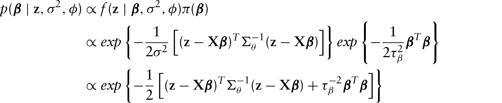
We follow the Bayesian approach for model estimation and prediction which is based on the posterior distribution for model parameters. The posterior distribution is obtained by the Bayes rule, which is given by $p (Θ ∣ z) \propto f (z ∣ Θ) π (Θ)$ , with $z$ the observed data and $Θ$ the unknown parameters. As $p (Θ ∣ z)$ is usually not obtained in closed form, stochastic simulation methods are often called for (Gamerman and Lopes, 2006). If Gaussianity is assumed for $Z (s)$ as in Equation (2.2), then the likelihood function for the spatial model without nugget effect is given by

f (z ∣ β, σ^{2}, θ) = (2 π)^{- n / 2} {|σ^{2} Σ_{θ}|}^{- 1 / 2} \exp \{- \frac{1}{2 σ^{2}} (z - μ)^{T} {Σ_{θ}}^{- 1} (z - μ)\},

(2.5)

that is, $z = (z_{1}, \dots, z_{n})^{T}$ follows an n-variate normal distribution with mean $μ = X β$ and covariance matrix $σ^{2} Σ_{θ}$ . To complete the Bayesian model, we specify a prior distribution for the parameters $β, σ^{2}, θ$ by assuming prior independence, that is, $π (β, σ^{2}, θ) = π_{1} (β) π_{2} (σ^{2}) π_{3} (θ)$ . We consider usual parametric non-informative priors $β \sim N_{n} (0, τ_{β}^{2} I_{n})$ with large values of $τ_{β}^{2}$ and $σ^{- 2} \sim Ga (a, b)$ with small values of $a$ and $b$ . For covariance matrix, we consider the exponential correlation function which depends on the range parameter $ϕ$ . We take into account that the prior on $ϕ$ is critically dependent of the scale of distances between locations. So, $ϕ \sim Ga (1, c / med (d))$ , with $med (d)$ representing the median of distances in the data.

Markov chain Monte Carlo (MCMC) methods are applied to estimate the posterior distribution $p (β, σ^{2}, θ ∣ z)$ through a Gibbs sampler scheme with Metropolis–Hastings step for $θ$ simulation, which considers a random walk proposal. Complete conditional distributions and more details about the MCMC scheme are given in Appendix 6.1.

For the Student-t spatial process, the likelihood function is given by

f (z ∣ β, σ^{2}, θ, ν) = \frac{Γ (\frac{ν + n}{2})}{Γ (\frac{ν}{2}) (ν π)^{n / 2} | σ^{2} Σ_{θ} |^{1 / 2}} {[1 + \frac{(z - μ)^{T} Σ_{θ}^{- 1} (z - μ)}{σ^{2} ν}]}^{- (ν + n) / 2},

(2.6)

with $Γ (\cdot)$ the gamma function, mean $μ = X β$ and covariance matrix $σ^{2} Σ_{θ}$ as in Equation (2.3). To complete the Bayesian model, the prior distributions are considered independent and the same as in the Gaussian case. The parameter $ν$ has a Jeffreys prior distribution as proposed in Fonseca et al. (2008) which is detailed in Appendix 6.2. The posterior samples for model parameters are obtained by the Metropolis–Hastings steps for $β, σ^{2}, θ$ and $ν$ which are based on random walk proposals, as detailed in Appendix 6.2.

For the Gaussian-log-Gaussian spatial process, we assume a mixing variable $λ_{i} \in R_{+}$ assigned to each observation $i = 1, \dots, n$ , which leads to a multivariate Gaussian distribution for $z$ conditional on $λ = (λ_{1}, \dots, λ_{n})$ . The resulting likelihood function is like that in (2.5) with $Σ_{θ}$ replaced by $Σ_{θ}^{★} = Λ^{- 1 / 2} Σ_{θ} Λ^{- 1 / 2}$ , where $Λ = Diag (λ_{1}, \dots, λ_{n})$ . To complete the Bayesian model, we specify for parameters $β, σ^{2}, θ$ the same priors considered for the Gaussian case, and for the parameter $ν$ we set a $GIG (0, δ, ι)$ , which for very small values (around 0.01) corresponds to near normality and large values (on the order of say 3) indicate very thick tails and $\ln (λ) \sim N_{n} (- \frac{ν}{2} 1, ν Σ_{θ})$ . The posterior samples for model parameters are obtained by the Gibbs algorithm with Metropolis–Hastings steps for $θ$ , $ν$ and $λ$ , which are based on random walk proposals. For a more elaborate algorithm, see Palacios and Steel (2006). Appendix 6.3 presents the prior distributions and posterior inference for the model parameters.

In the context of prediction, let $z = (z_{0}, z_{s})$ where $z_{0}$ represents out-of-sample observations for which we want to obtain predictions and $z_{s}$ represents the observations used for parameter estimation. Predictive distributions are obtained in closed form for all considered models. For the GM the conditional distributions remain Gaussian with mean and variance given by

E [Z_{0} ∣ z_{s}] = x_{0}^{T} β + Σ_{0 s} Σ_{ss}^{- 1} (z_{s} - x_{s}^{T} β)

(2.7)

Var [Z_{0} ∣ z_{s}] = σ^{2} Σ_{00} - σ^{2} Σ_{0 s} Σ_{ss}^{- 1} Σ_{s 0},

(2.8)

where we have partitioned

Σ_{θ} = (\begin{matrix} Σ_{00} & Σ_{0 s} \\ Σ_{s 0} & Σ_{ss} \end{matrix})

For the STM, the conditional distributions remain Student-t with degrees of freedom $ν_{0 ∣ s} = ν + d_{s}$ , and with mean and variance given by

E [Z_{0} ∣ z_{s}] = x_{0}^{T} β + Σ_{0 s} Σ_{ss}^{- 1} (z_{s} - x_{s}^{T} β),

(2.9)

Var [Z_{0} ∣ z_{s}] = ξ (s) [σ^{2} Σ_{00} - σ^{2} Σ_{0 s} Σ_{ss}^{- 1} Σ_{s 0}],

(2.10)

where

ξ (s) = \frac{ν + (z_{s} - x_{s}^{T} β)^{T} Σ_{ss}^{- 1} (z_{s} - x_{s}^{T} β)}{ν + d_{s}},

where $d_{s}$ represents the dimension of vector $z_{s}$ . Notice that by letting $ν$ go to infinity, we can recover the Gaussian conditional covariance structure. See Roislien and Omre (2006) for more details.

For the GLG case and conditional on the mixing variables $λ$ , the predictive distributions are analogous to (2.7) and (2.8) with $Σ_{θ}$ replaced by $Σ_{θ}^{★}$ . The mixing variables $λ$ are considered latent variables and are sampled in the MCMC algorithm. Details are given in Appendix 6.3.

3 Outlier detection in spatial modelling

In this section, we describe three approaches to outlier detection in spatial modelling: the posterior probability computation of a large residual, predictive techniques such as the predictive concordance and hypothesis testing for the latent mixing variables. In this context, techniques used for univariate data are extended to spatial data analysis.

3.1 Bayesian residual analysis

Definition 3.1 Consider $Z = (Z (s_{1}), \dots, Z (s_{n}))$ observations at $n$ spatial locations of the spatial process ${Z (s), s \in D}$ as defined in Equation (2.1) such that $Z ∣ β, σ^{2}, Λ \sim N_{n} (X β, σ^{2} (Λ^{- 1 / 2} Σ_{θ} Λ^{- 1 / 2}))$ , with $Λ = diag (λ)$ . Then the standardized Bayesian spatial residual (SBSR) for the mixture model without nugget effect is

r = σ^{- 1} Λ^{1 / 2} Σ_{θ}^{- 1 / 2} (Z - X β) .

(3.1)

If the errors have Gaussian distribution, then approximately $95 %$ of the individual residuals are expected to be in the interval $[- 2, 2]$ . If an observation is out of this interval, there is some evidence that this observation could be an outlier. In order to detect outlying observations, Chaloner and Brant (1988) defined the posterior probability that an observation is an outlier as $p_{i} = P (| r_{i} | > t ∣ z)$ . According to Chaloner and Brant (1988), the value of $t$ can be chosen so that the prior probability of no outliers is large, say 0.95, in which case the constant $t$ is chosen to be $Φ^{- 1} (0.5 + 0.5 (0 . 95^{1 / n}))$ , where $Φ$ represents the cumulative distribution function. Any observation with posterior probability of being an outlier larger than the prior probability $2 Φ (- t)$ would be suspect. In a context of binary regression, Albert and Chib (1995) and Souza and Migon (2010) considered $t = 0.75$ .

In the geostatistical setting, we set the value of $t$ to different constants and verify by simulation for several scenarios how the mixture process is sensitive to this choice. The usual expectation is that not all values used for classical regression models will have good performance in the correlated data context.

Furthermore, we investigate the joint posterior probability of two or more observations being outliers. This is a phenomenon which is expected in spatial applications. In particular, due to spatial correlation of observations and smoothness of the spatial process, two observations, for example, which are close together are expected to have large errors if there is a mechanism causing outliers in the spatial region where these two observations are located. Thus, the joint posterior probability that the pair $(r_{i}, r_{j})$ is a regional or multiple outlier is

p_{ij} = P (| r_{i} | > t, | r_{j} | > t ∣ z) .

(3.2)

In particular, the variance process $1 / λ (s)$ in the GLG model is considered to be correlated with $\ln (λ) ∣ ν \sim N_{n} (- \frac{ν}{2} 1, ν Σ_{θ})$ . Thus, if an individual outlier is detected, then this indicates that observations in the nearby neighbourhood are potential outliers. This can be verified by computing $p_{ij}$ . Fonseca and Steel (2011) extended this proposal by allowing for independent outlying observations through individual nugget effects for each location. This approach is not discussed here, since replicates in time would be required for parameter estimation.

3.2 Predictive approach

An alternative definition of an outlier was given by Gelfand (1996). An observation is said to be aberrant or discrepant if it is in the tails of the predictive posterior distribution. The author defined the predictive concordance for observed value $z_{i}$ as

{pc}_{i} = P (z^{rep} > z_{i}) = \int_{z_{i}}^{\infty} p (z^{rep}) {dz}^{rep},

(3.3)

with $z^{rep}$ an imaginary observation and $p (z^{rep})$ the predictive distribution of $z^{rep}$ . This measure is similar to the Bayesian p-value. According to Gelfand (1996), any observation which is in the $2.5 %$ tail of $p (z^{rep})$ should be considered an outlier. The percentage of outliers in the data should be smaller than $(100 - C) %$ , where $C %$ is the predictive concordance. Gelfand (1996) suggested $95 %$ predictive concordance as the threshold for model adequacy.

Note that the ${pc}_{i}$ is computed based on the full predictive distribution, but, to check whether $z_{i}$ is an outlier, it actually uses $z_{i}$ to obtain the predictive distribution. Thus, the model might predict this observation better than it would if $z_{i}$ was not in the data. The leave-one-out predictive distribution obtained by removing $z_{i}$ from the data might give better information about model performance in predicting $z_{i}$ . Gelfand (1996) proposed the conditional predictive ordinate (CPO)

{cpo}_{i} = p (z_{i} | z_{(i)}) = \int p (z_{i} | θ) p (θ | z_{(i)}) d θ,

(3.4)

where $z_{i}$ represents an observed value from $z$ , $z_{(i)}$ represents the vector $z$ without $z_{i}$ and $θ$ is the parameters of model. Note that $p (z^{rep} | z_{(i)})$ represents the predictive density of a new observation given the dataset that does not include $z_{i}$ . Values of ${cpo}_{i}$ close to zero suggest that observation $i$ is a potential outlier. Petit (1990) commented that although the ${cpo}_{i}$ could be used as a surprise index, it might return similar values for all observations, failing to identifying outlying observations. In these situations, Petit (1990) suggested a new measure called ratio ordinate measure (ROM), which is the CPO standardized by $\max {p (z^{rep} | z_{(i)})}$ . This measure aims at giving more realistic indications of outliers in a dataset. Following the ideas based on predictive distributions and predictive concordance, here we propose a measure for spatial data which is based on cross-validation ideas. Definition The p-value from conditional predictive ordinate is defined as

{CPOp}_{i} = P (z^{rep} > z_{i} | z_{(i)}) .

(3.5)

The proposed measure is similar to the predictive concordance, but it leaves $z_{i}$ out of the dataset used for parameter estimation. This proposal checks whether the observed value $z_{i}$ is in accordance with the predictive distribution that was obtained by excluding $z_{i}$ from the dataset. For this measure, values of $z_{i}$ in either tail of the predictive distribution will indicate that $z_{i}$ is an outlier.

3.3 Savage–Dickey ratio test

A different approach to outlier detection considers inference directly in the mixing process $λ (s)$ , $s \in D$ . Thus, $λ (s_{k})$ close to one indicates that the observation at location $s_{k}$ is not an outlier. So, the model that considers $λ (s_{k}) = 1$ could be compared to the model which considers free $λ (s_{k})$ . This model comparison can be done through Bayes factors after fitting both models to the data. An alternative to fitting both models and then computing the Bayes factor (Kass and Raftery, 1995) is to consider only the model with free $λ (s_{k})$ and the Savage–Dickey density ratio to approximate the Bayes factor for the hypothesis that $λ (s_{k}) = 1$ versus $λ (s_{k}) \neq 1$ . The Savage–Dickey density ratio was proposed by proposed by Dickey (1971) and can be used when the restriction in the parameter being tested in the null hypothesis is not on the boundary of the parameter domain. According to Palacios and Steel (2006), this hypothesis testing is useful to indicate outliers in the data or regions with larger variability in space. The resulting approximation for the Bayes factor for each location $s_{k}$ is given by

R_{k} = {\frac{p (λ (s_{k}) | z)}{p (λ (s_{k}))}}_{| λ (s_{k}) = 1},

(3.6)

with the ratio $R_{k}$ being favourable to the model with $λ (s_{k}) = 1$ and all the other $λ$ free against the model with free $λ (s_{k})$ . Thus, small values of $R_{k}$ (much smaller than 1) will indicate outliers. (Kass and Raftery, 1995) give some guidelines for interpretation of Bayes Factors. According to the authors, values of $R_{k}$ smaller than 0.10 give strong evidence that $λ (s_{k}) \neq 1$ . Values between 0.1 and 0.3 give substantial evidence that $λ (s_{k}) \neq 1$ , while values between 0.3 and 1 give some evidence but are not very conclusive.

4 Applications

4.1 Simulated dataset

In this subsection, the Gaussian, Student-t and Gaussian-log-Gaussian models presented in Section 2.1 are considered for the identification of outliers in contaminated datasets. For that purpose, we perform spatial residual analysis and compute the predictive concordance measure and the Bayes factor hypothesis test for outlier detection. Then we compare the methods regarding their ability to detect aberrant observations in geostatistical data. The data considered for simulation are realizations from a Gaussian processes, which after contamination presents outliers. West (1984) commented that contaminated datasets, simulated originally from the Gaussian distribution and then contaminated to characterize aberrant observations, are a useful tool to evaluate the performance of robust models.

Assume that $Z (s)$ is a spatial process in D. We simulated 50 datasets, each containing $n = 30$ observations $z = (z (s_{1}), \dots, z (s_{n}))^{'}$ from a multivariate Gaussian distribution with mean $μ_{i} = μ (s_{i}) = β_{0} + β_{1} {lat}_{i} + β_{2} {long}_{i}$ and covariance matrix $σ^{2} Σ_{θ}$ with $Σ_{θ (ij)} = \exp {- | | s_{i} - s_{j} | | / ϕ}$ , with ${lat}_{i}$ and ${long}_{i}$ the latitude and longitude of spatial location $i$ , respectively. The parameter values considered for simulation were $β_{0} = 6.716, β_{1} = 2.7, β_{2} = - 1.808$ , $σ^{2} = 1.0$ and $ϕ = 0.61$ .

Three scenarios were evaluated for each of the 50 replicates: no contamination (a), weak contamination (b) and moderate contamination (c). Observations in the weak contamination scenario were contaminated summing random increments $u σ$ with $σ$ the observational standard deviation and $u \sim Uniform (1, 3.5)$ for observations 1 and 20 and $u \sim Uniform (1, 2.5)$ for observation 6. In the moderate scenario, the increments were $u \sim Uniform (1, 3.5)$ for observations 1, 15, 16, 20, 30, $u \sim Uniform >(1, 2.5)$ for observation 6 and $u \sim Uniform (1, 6.5)$ for observation 29. 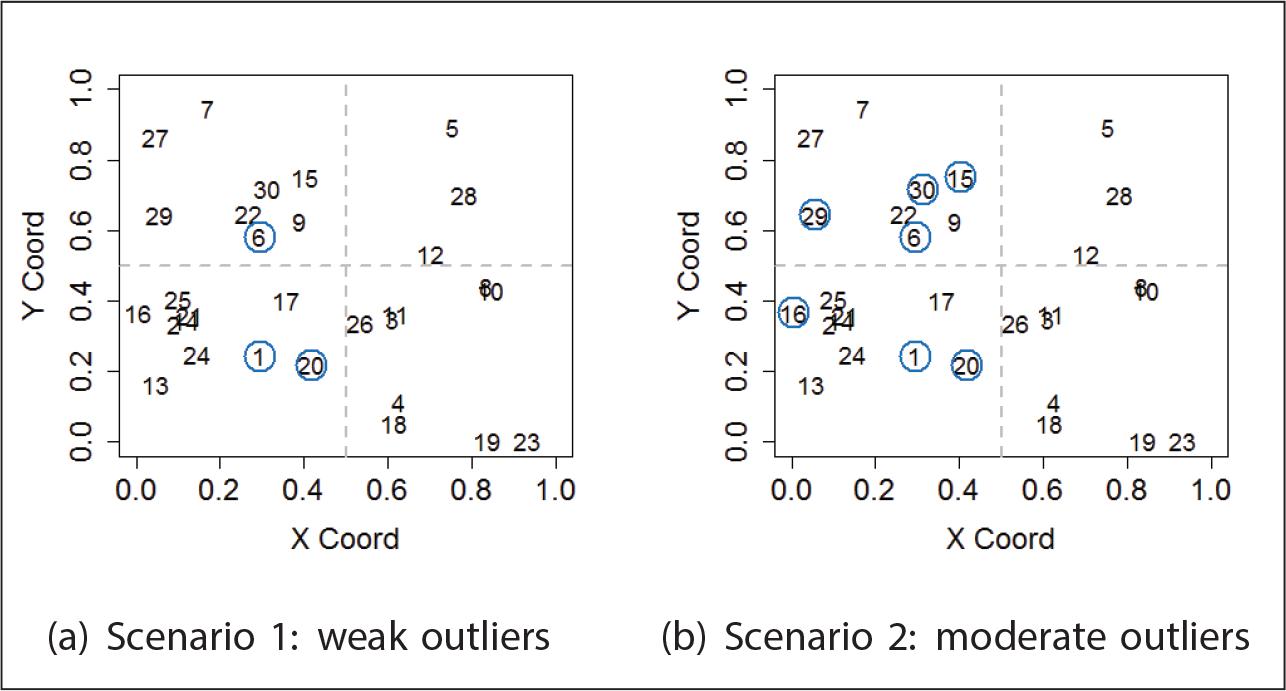The locations considered for data simulation in scenarios 2 and 3 are presented in Figure 1. Note that some of the contaminated locations are neighbours in space.

Figure 1:

Spatial locations considered for data simulation in the contaminated data scenarios. Locations in blue circles represent the contaminated locations in each scenario. Plot (a) represents scenario 2 and (b) represents scenario 3

Parameter estimation and prediction follow the Bayesian paradigm as presented in subsection 2.2. The chains for the simulated parameters have burn-in of 50 000 and lag of 30 with resulting posterior sample size of 5 001. Convergence was checked using the coda package (Plummer et al., 2006). The MCMC algorithm resulted in acceptance rates in the vicinity of 25% to 45% for each block of parameters. The prior distributions used for all models were $β \sim N_{n} (0; 10^{4} I_{n})$ , $σ^{- 2} \sim G (0.001; 0.001)$ and $ϕ \sim G (1; 0.92 / med (d))$ . For the STM, we considered the Jeffreys prior for $ν$ as detailed in Appendix 6.2. For the GLGM, $ν \sim GIG (0; 0.75; 6)$ and $λ ∣ ϕ, ν \sim LN (- \frac{ν}{2} 1; ν Σ_{θ})$ . The computational time for single MCMC runs of GM, STM and GLGM was about 273 seconds, 304 seconds and 1 460 seconds, respectively, using a machine with specification Intel core i5. 3.10 GHz, RAM 8GB, 64 bits.

Table 1:

Percentage of right classification based on posterior residual probabilities of outliers $p (r_{i} > t_{k} ∣ z), k = 1, 2, 3$ for replicated datasets. Non and cont mean non-contaminated and contaminated observations, respectively

		GM			STM			GLGM
		$p (t_{1})_{i}$	$p (t_{2})_{i}$	$p (t_{3})_{i}$	$p (t_{1})_{i}$	$p (t_{2})_{i}$	$p (t_{3})_{i}$	$p (t_{1})_{i}$	$p (t_{2})_{i}$	$p (t_{3})_{i}$
Scenario 1	non	0.385	0.936	0.999	0.384	0.935	0.999	0.369	0.931	0.999
	cont	1.000	0.973	0.827	1.000	0.960	0.827	1.000	0.953	0.940
Scenario 2	non	0.535	0.978	1.000	0.470	0.958	0.999	0.238	0.951	1.000
Scenario 3	cont	0.923	0.611	0.337	0.951	0.649	0.386	0.983	0.891	0.711
	non	0.384	0.913	0.996	0.335	0.867	0.974	0.203	0.922	0.978

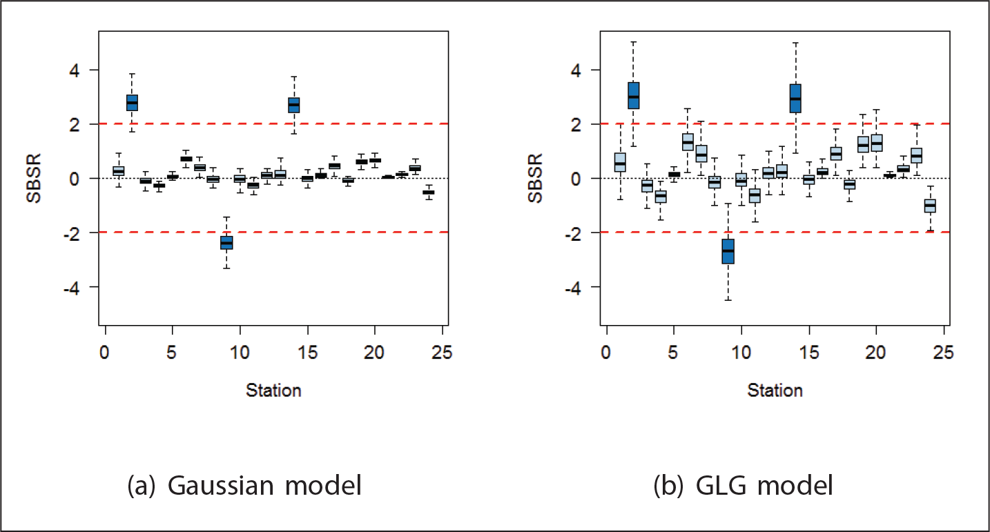
We now present a summary of the results for the 50 replicated datasets to illustrate the usefulness of the proposed tools for spatial outlier detection. The results of the simulated study are used to define benchmarks for hypothesis tests along the applications. Figure 2 presents the spatial residuals for one selected illustrative dataset. For scenario 1, the residuals behaved as expected and no aberrant observation is identified. For scenario 2, all models are able to detect observations 1 and 20 as potential outliers, but only the GLGM identifies observation 6 as a potential outlier. For scenario 3, all models are able to detect observations 1, 15 and 20 as potential outliers, but only the GLGM identifies observations 6, 16, 29 and 30 as outliers.

Figure 2:

Note: For references to colour, please see the article online.

To classify each observation as an outlier, we computed

p_{i} (| r_{i} | > t ∣ z)

, which depends on the threshold

t

. The threshold choice is crucial and was determined by our simulated study presented in Table 1, which shows the percentage of correct classification of outliers for the 50 replicated datasets. This measure indicates that threshold

t_{1}

classifies too many observations as outliers with less than

40 %

right classification. On the other hand, threshold

t_{2}

has large percentage of correct classifications for both contaminated (cont) and non-contaminated (non) observations. Threshold

t_{3}

has a worse performance than threshold

t_{2}

. Therefore, we suggest the use of threshold

t_{2}

as a benchmark for outlier detection.

In the context of spatial analysis, the identification of neighbouring observations which are outliers is of great interest. Table 2 confirms that only GLGM is able to correctly identify multiple outliers. Indeed, threshold $t_{2}$ give very large probabilities of correct classification for the contaminated pair of outliers for the GLGM. Note that GM and STM are not flexible enough to identify outliers in a neighbouring region, resulting in very low probabilities of outliers for several pairs of contaminated observations for threshold $t_{2}$ in particular for scenario 3. For instance, the pair (1,15) of contaminated observation has outlier probabilities of 0.28, 0.10 and 0.84 for the GM, STM and GLGM, respectively. Threshold $t_{1}$ is not meaningful, since it classifies as outliers many pairs which were not contaminated.

Table 2:

Results in percentage for posterior residual probabilities of multiple outliers for replicated datasets

		GM			STM			GLGM
	obs.	$p (t_{1})_{i}$	$p (t_{2})_{i}$	$p (t_{3})_{i}$	$p (t_{1})_{i}$	$p (t_{2})_{i}$	$p (t_{3})_{i}$	$p (t_{1})_{i}$	$p (t_{2})_{i}$	$p (t_{3})_{i}$
	1,6	0.20			0.20			0.06
Scenario 1	1,20	0.12			0.14			0.10
	6,14	0.16	0.02		0.14	0.02		0.16	0.02
	1,6	1.00	0.98	0.52	1.00	0.78	0.44	0.98	0.94	0.62
	1,20	1.00	0.76	0.40	0.98	0.74	0.38	0.98	0.80	0.42
Scenario 2	6,20	1.00	0.94	0.70	1.00	0.96	0.74	1.00	0.98	0.78
	1,6,20	1.00	0.74	0.48	0.98	0.76	0.28	1.00	0.84	0.56
	1,6	0.96	0.82	0.26	1.00	0.84	0.28	0.98	0.88	0.54
	1,20	0.98	0.86	0.20	1.00	0.90	0.26	1.00	0.90	0.42
Scenario 3	6,20	1.00	0.90	0.24	1.00	0.84	0.32	0.98	0.74	0.44
	1,15	0.76	0.28	0.02	0.88	0.10	0.04	0.86	0.84	0.54
	15,30	0.70	0.14		0.80	0.06		0.98	0.80	0.54
	6,15,30	0.78	0.26		0.82	0.28	0.02	0.96	0.66	0.50

Note: Percentages equal $10^{- 2}$ are omitted from the table.

Furthermore, the predictive measures were computed for the contaminated scenarios. The measure ${cpo}_{i}$ has poor performance, since the values are very often low and not meaningful, as already discussed in Petit (1990). This was confirmed in the simulated study with 50 replicated datasets as presented in Table 3. This measure apparently detects the contaminated observations as potential outliers, but it detects many other observations which are not actually contaminated. In particular for STM, the CPO values are often very small indicating outliers for non-contaminated observations. The measures ${pc}_{i}$ and ${CPOp}_{i}$ correctly classify the contaminated and non-contaminated observations.

Table 3:

Percentage of right classification based on predictive measures ${pc}_{i}$ , ${cpo}_{i}$ and ${CPO}_{p_{i}}$ for replicated datasets

		GM			STM			GLGM
		${pc}_{i}$	${cpo}_{i}$	${CPOp}_{i}$	${pc}_{i}$	${cpo}_{i}$	${CPOp}_{i}$	${pc}_{i}$	${cpo}_{i}$	${CPOp}_{i}$
Scenario 2	cont	0.987	0.913	0.920	0.940	0.973	0.627	0.993	1.000	0.907
	non	1.000	0.987	1.000	1.000	0.412	1.000	1.000	0.143	0.997
Scenario 3	cont	0.697	0.537	0.691	0.594	0.906	0.454	0.860	0.991	0.800
Scenario 3	non	1.000	0.957	1.000	1.000	0.400	1.000	1.000	0.023	1.000

We computed the Savage–Dickey density ratio to test the hypothesis of $λ_{i} = 1$ (observation $i$ is not an outlier) versus $λ_{i} \neq 1$ (observation $i$ is an outlier). The decision depends on the threshold choice for $R_{i}$ as shown in Table 4 for the 50 replicated datasets. The study indicated that using the threshold $R_{i} < 0.1$ for classification of outliers is too conservative and fails to identify the outliers in scenarios 2 and 3. On the other hand, thresholds between 0.1 and 0.3 correctly indicates the outlying observations with probabilities of $93 %$ and $85 %$ for scenarios 2 and 3, respectively.

Table 4:

Percentage of correct outlier indications by the Savage–Dickey density ratio $R_{i}$ for hypothesis testing in favour of $λ_{i} = 1$ for the 50 replicated datasets. Values of $R_{i}$ for outlier identification are $R_{i}^{(a)} < 0.1; R_{i}^{(b)} < 0.3; R_{i}^{(c)} < 1$

	Scenario 2			Scenario 3
	$R_{i}^{(a)}$	$R_{i}^{(b)}$	$R_{i}^{(c)}$	$R_{i}^{(a)}$	$R_{i}^{(b)}$	$R_{i}^{(c)}$
cont	0.813	0.933	0.947	0.649	0.849	0.920

Overall, the analysis of residuals highlights the main potential outliers in the data. The plot of residuals correctly indicates no outlier in the Gaussian data scenario for all models. However, the plot fails to indicate outliers for non-robust models. This might be due to inflation of variance of the Gaussian and Student-t models, which are unable to accommodate different tail behaviours across space. The posterior probability of large random errors gives a very precise indication of outliers in the Gaussian-log-Gaussian case. The threshold $t_{1}$ is very small and allows for too many observations to be classified as outliers, leading to only $40 %$ correct classification. Threshold $t_{2}$ gives a very reasonable percentage of right classification for the 50 replicated datasets for both univariate and pairwise outlier identification and is suggested as a benchmark for practitioners. Regarding the predictive measures, the ${pc}_{i}$ and ${CPO}_{p_{i}}$ correctly indicate the contaminated observations as potential outliers for most of the replicated datasets. The Savage–Dickey density ratio $R_{i}$ is a powerful tool for outlier detection and values of $R_{i} \in (0.1, 1)$ are suggested for hypothesis testing.

4.2 Wind speed in Brazil

In recent years, the use of wind energy has increased rapidly in Brazil, with the main wind farms being located in the South and Northeast regions. Nowadays, wind power corresponds to approximately $5 %$ of the total electricity generated in Brazil. However, this will tend to increase in the next few years. The government's aim is for wind power to account for 10% in 2019. In particular, several turbines have been tested in the state of Minas Gerais. In this article, we analyse data from wind turbines to detect regional outliers, which would correspond to potentially interesting regions for wind power exploitation in Minas Gerais. The electrical potential obtained from wind is a cubic function of wind speed. Thus, detection of wind speed values is of interest in the analysis of wind power capacity. In the management of wind power generation and demand for electrical power, the adequate measurement of uncertainty in the prediction of wind speed is of great interest. In that context, this section investigates the detection of outliers and goodness of fit for wind speed spatial modelling. The data analysed were obtained from CEMIG, a company operating in the electrical sector in Brazil. The turbines considered were installed in the Espinhaço and Rio Verde regions of Minas Gerais. Figure 3 presents the region of interest and the numbered wind turbines considered in this analysis. The dataset contains the daily mean for 24 wind turbines on 13 August 2001.

Figure 3:

Turbines in Espinhaço and Rio Verde regions of the state of Minas Gerais

The spatial mean was adjusted considering the latitude, longitude and altitude as covariates. The mixture models considered were the Gaussian and Gaussian-log-Gaussian models, as presented in subsection 2.1. Posterior inference for model parameters was performed as discussed in subsection 2.2. The prior distributions considered were $σ^{- 2} \sim G (0.1; 0.1)$ , $ϕ \sim G (0.5; 0.5)$ in both GM and GLGM and $ν \sim G (1; 5)$ and $λ ∣ ϕ, ν \sim LN (- \frac{ν}{2} 1; ν Σ_{θ})$ for GLGM. The convergence of the chains was evaluated by coda as in the simulated study. Figure 4 shows the posterior spatial residuals, indicating observations 2, 9 and 15 as potential outliers for both models.

Table 5 presents the probability of outliers for thresholds $t_{1}$ , $t_{2}$ and $t_{3}$ . Observations 2, 9 and 14 have large probability of being outliers based on threshold $t_{2}$ for both models.

Figure 4:

Standard Bayesian spatial residual posterior distribution

Table 5:

Standardized residuals and posterior probabilities of outliers, $p_{i} (| r_{i} | > t | z)$ . Large values of $p (t_{k})_{i}$ indicate outliers. Boldface observations represent the observations classified as outliers

	GM			GLGM
$i$	$p (t_{1})$	$p (t_{2})$	$p (t_{3})$	$p (t_{1})$	$p (t_{2})$	$p (t_{3})$
2	1.000	0.977	0.227	1.000	0.985	0.462
9	1.000	0.857	0.033	1.000	0.861	0.287
14	1.000	0.966	0.169	0.999	0.907	0.417
24	0.0078			0.780	0.015

Note: Posterior probabilities smaller than $10^{- 3}$ are omitted from the table.

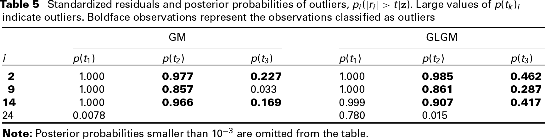
Table 6 presents the predictive approaches ${pc}_{i}$ , ${cpo}_{i}$ and ${CPOp}_{i}$ . Observe that CPOp identifies observations 2, 9 and 14 as outliers for both Gaussian and GLG models. Observation 24 is in the tail of the predictive distribution for the GLG model while the Gaussian model does not identify this observation not even as a potential outlier. Indeed, this difference for observation 24 could be confirmed from the residuals for these models. For the Gaussian residual, the distribution is very concentrated inside the limits $[- 2, 2]$ while in the GLG model, the standard bayesian spatial residual (SBSR) distribution is in the boundary of this region, as shown in Figure 4. Furthermore, note that for observation 24, the ${CPOp}_{i}$ indicates an potential outlier and ${pc}_{i}$ and ${cpo}_{i}$ do not. This highlights the advantage of ${CPOp}_{i}$ which removes the observation $i$ from the data to obtain the predictive distribution. This removal might be crucial for outlier identification in application with few locations such as this one. As already indicated from the replicated data study, the ${cpo}_{i}$ give very low values for most observations failing to identify potential outliers.

Table 6:

Predictive measures ${pc}_{i}$ , ${cpo}_{i}$ , ${CPOp}_{i}$ for some observations in the sample. Boldfaced observations represent the observations classified as outliers

	GM			GLGM
obs	${pc}_{i}$	${cpo}_{i}$	${CPOp}_{i}$	${pc}_{i}$	${cpo}_{i}$	${CPOp}_{i}$
2	0.010		0.010	0.007		0.005
5	0.416	0.081	0.369	0.306		0.102
9	0.973		0.982	0.979		0.988
11	0.585	0.085	0.638	0.688		0.878
14	0.010		0.007	0.011		0.009
24	0.700	0.064	0.772	0.832		0.960

Note: Values smaller than $10^{- 4}$ are omitted from the table.

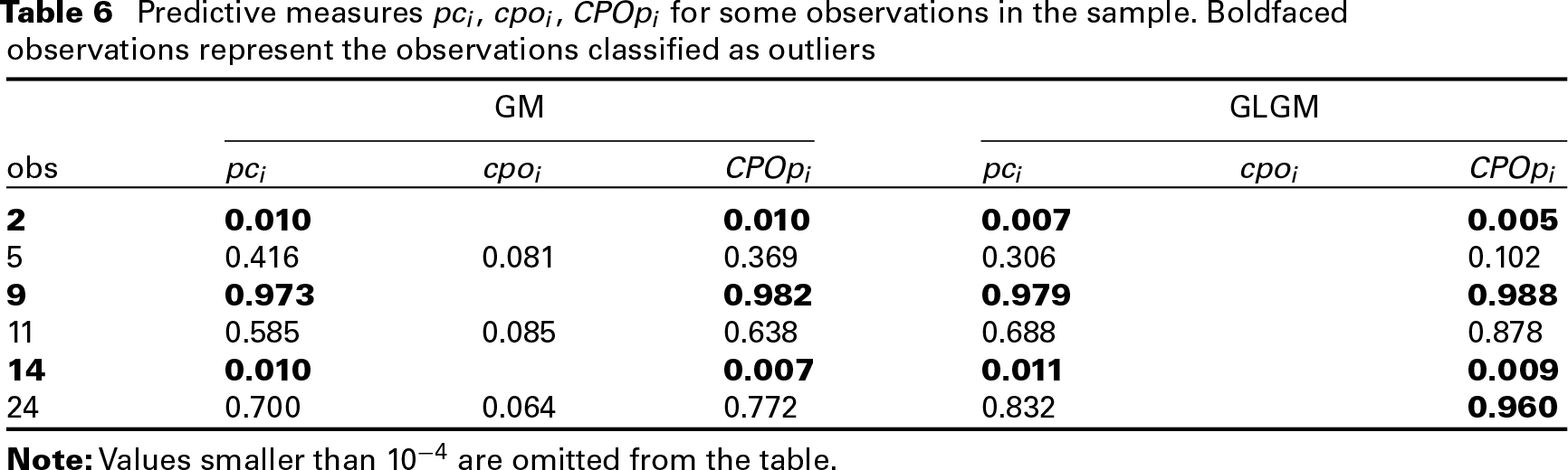
Table 7 presents the Bayes factor based on the Savage–Dickey approximation. Observations 2, 9 and 14 are indicated as potential outliers by the Bayes factor test with $R_{i}$ values 0.065, 0.236 and 0.134, respectively. Note that the uncertainty in this application is quite large in the estimation of $λ$ . This is due to the sample size which is small in this application. According to Fonseca and Steel (2011), temporal observations might be required for good estimation with mixed latent variables when the spatial sample size is small.

Table 7:

Savage–Dickey density ratio $R_{i}$ for hypothesis testing in favour of $λ_{i} = 1$ . Boldface observations represent evidence of outliers ( $R_{i} < 0.3$ )

obs.	$E (λ_{i} \| z)$	$SD (λ_{i} \| z)$	$R_{i}$
2	0.247	0.164	0.065
5	1.082	0.729	1.050
9	0.264	0.182	0.236
11	1.076	0.837	0.915
14	0.241	0.168	0.134
24	0.729	0.459	0.924

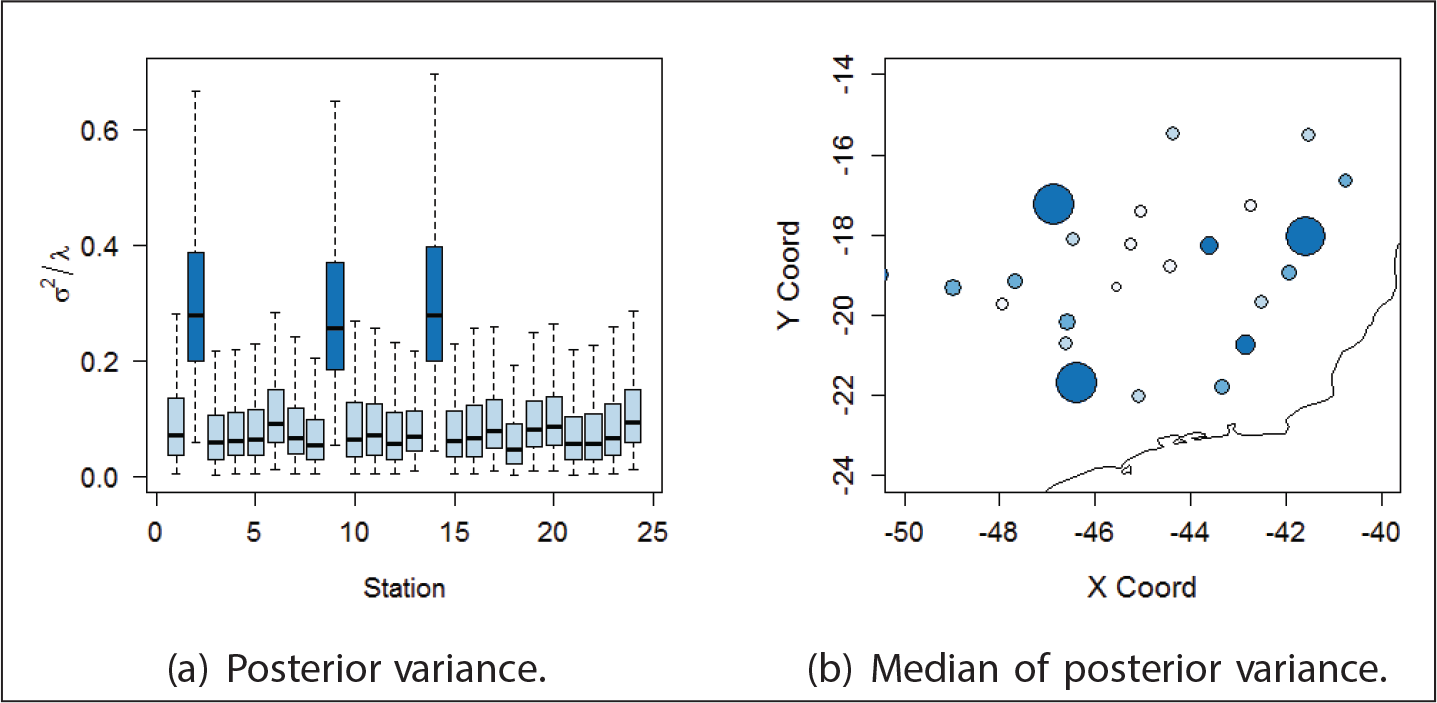
The three observations classified as outliers in this application are within the boundaries of the spatial region considered. Further investigation should be performed to explain the larger residuals obtained for these locations. Figure 5 presents the posterior variance for each location defined by $σ^{2} / λ_{k}$ in the GLGM. The three largest variances correspond to the observations indicated as outliers by most of the methods tested in this application: observations 2, 9 and 14. Observation 9 presents very large negative residuals, indicating weaker winds than the average. On the contrary, observations 2 and 14 exhibit very large wind speeds. This is an important result, since wind power generation is related to the cubed wind speed, leading to even large impacts for eolic energy prediction and generation.

Figure 5:

Note: For reference to colour, please see the article online.

5 Conclusions

The idea that the Student-t process would result in robust to outliers is misleading since the degree of freedom is the same in all spatial locations, leading to inflation in the global variance. Thus, this model does not allow for actual detection of regions with aberrant observation in spatial data. These ideas were discussed in Breusch et al. (1997) and Palacios and Steel (2006). This work contributes by presenting simulation for spatial contaminated datasets and obtaining no detection of most of outliers in the data using the Student-t model. The Student-t process for spatial data was not able to detect outliers either by marginal probabilities or multiple detection procedures. The GLG mixture process, on the other hand, indicated the outliers in all simulated scenarios for all detection tools presented in this work. The residual analysis presented here is purely spatial in the sense that the mixture process is considered in space only. Fonseca and Steel (2011) considered a mixture model in space–time, which is not exploited in this work.

The spatial Bayesian residuals, the proposed cross-validation p-value and the Savage–Dickey density were investigated in this study. Specifically, the probability of a large random error is a useful tool for outlier detection, although it depends on the threshold specification. Our simulated study with replicated datasets indicated that threshold $t_{2}$ gives the best outlier classification rates for all scenarios, being preferred to thresholds $t_{1}$ and $t_{3}$ , which have been used in the literature in non-correlated data analysis. The CPO failed to identify outliers in our simulated study and wind data analysis. As an alternative, we proposed the p-value based on the CPO, which was able to correctly detect aberrant observations in the spatial data. The proposed CPOp is advantageous compared to the predictive concordance since it removes the observation under study from the dataset in the estimation and prediction procedure. In the wind data illustration, the CPOp was able to identify outliers which were not detected by the predictive concordance. This is explained by the small sample size in this application, so that removing one observation has a strong effect in the resulting predictive distribution. In the context of hypothesis testing, the Savage–Dickey test depends on the threshold definition to reach a conclusion. As a general rule, values between 0.1 and 1 gave reasonable classification rates in our simulated study.

Often in statistical data analysis, tests and inferences are performed regarding model parameters based on models which may not be adequate for the data. In order to add flexibility to the analysis, general models such as the mixture spatial models accommodate more general data behaviours. In this context, there is a growing literature which aims to loosen the usual model assumptions. For instance, Klein et al. (2015) proposed using of distributional regression, which allows for more flexibility in complex response distributions. Besides that, other techniques can be considered and extended to accommodate spatially correlated data such as quantile regression (Reich et al., 2011).

In the direction of model criticism and outlier detection, the cross-validation method is a powerful tool to assess the goodness of fit of spatial models and is an interesting approach for future investigation. From the Bayesian point of view, various authors have suggested the use of cross-validation. (See Stern and Cressie, 2000; Alqallaf and Gustafson, 2001; Vehtari and Lampinen, 2002; Marshall and Spiegelhalter, 2003; Vehtari et al., 2017). This direction will be pursued in future research.

Supplementary materials

Supplementary materials for this article are available from http://www.statmod..

Acknowledgements

We thank the referees and the editor for helpful comments. This work was part of the Master’s dissertation of Viviana GR Lobo under the supervision of TCO Fonseca.

Declaration of conflicting interests

The authors declared no potential conflicts of interest with respect to the research, authorship and/or publication of this article.

Funding

Lobo benefited from a scholarship from Conselho de Aperfeiçoamento de Pessoal de Nível Superior (CAPES), Brazil. TCO Fonseca was partially supported by Conselho Nacional de Desenvolvimento Científico e Tecnológico (CNPq).

Appendix

A1 Markov Chain Monte Carlo sampler

The prior distributions considered for the parameters, the complete conditional distributions and proposal densities used in the MCMC algorithm are detailed as follows.

A1.1 Gaussian Bayesian model

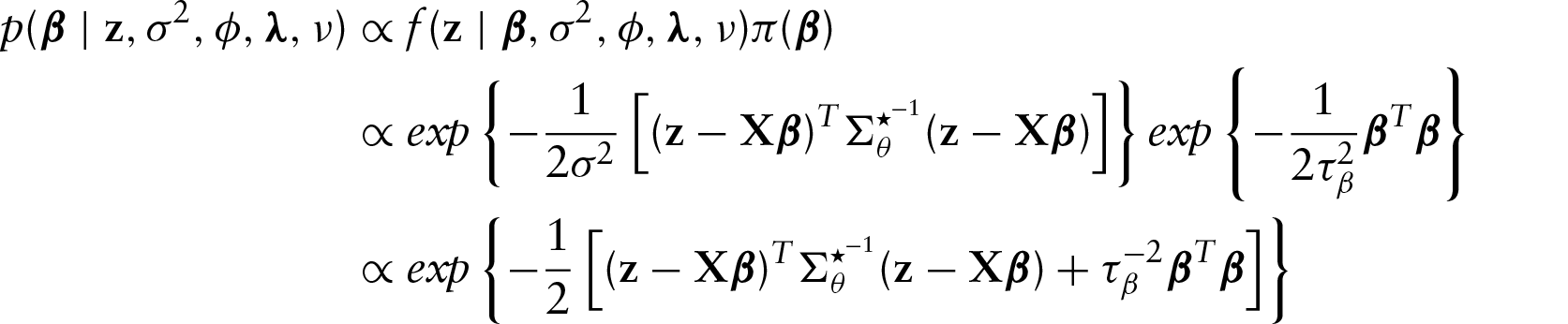
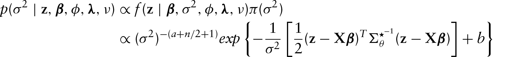
Consider the likelihood given in Equation (2.5) with exponential correlation function and covariance matrix $σ^{2} Σ_{θ (ij)} = σ^{2} \exp \{- | | s_{i} - s_{j} | | / ϕ\}$ , $i, j = 1, \dots, n$ .

$β \sim N_{n} (0, τ_{β}^{2} I_{n})$ , $τ_{β}^{2} > 0$ . Thus,

\begin{matrix} p (β ∣ z, σ^{2}, ϕ) & \propto & f (z ∣ β, σ^{2}, ϕ) π (β) \\ \propto & \exp \{- \frac{1}{2 σ^{2}} [(z - X β)^{T} Σ_{θ}^{- 1} (z - X β)]\} \exp \{- \frac{1}{2 τ_{β}^{2}} β^{T} β\} \\ \propto & \exp \{- \frac{1}{2} [(z - X β)^{T} Σ_{θ}^{- 1} (z - X β) + τ_{β}^{- 2} β^{T} β]\} \end{matrix}

The conditional distribution of $β ∣ z, σ^{2}, ϕ \sim N_{n} (μ_{1}, Σ_{1})$ with $Σ_{1} = (X^{T} Σ_{θ}^{- 1} {X + τ_{β}^{- 2} I_{β}^{- 1})}^{- 1}$ and $μ_{1} = Σ_{1} (X^{T} Σ_{θ}^{- 1} z)$ .

$σ^{- 2} \sim Ga (a, b)$ , $a, b > 0$ . Thus,

\begin{matrix} p (σ^{2} ∣ z, β, ϕ) & \propto & f (z ∣ β, σ^{2}, ϕ) π (σ^{2}) \\ \propto & (σ^{2})^{- (a + n / 2 + 1)} \exp \{- \frac{1}{σ^{2}} [\frac{1}{2} (z - X β)^{T} Σ_{θ}^{- 1} (z - X β)] + b\} \end{matrix}

The conditional distribution of $σ^{2} ∣ z, β, ϕ \sim Ga (a + \frac{n}{2}, \frac{1}{2} (z - X β)^{T} Σ_{θ}^{- 1} (z - X β) + b)$ .

$ϕ \sim Ga (1, c / med (d))$ , with $c > 0$ and $med (d)$ the median distance in the observed data. The proposed density in the MCMC sampler is

\ln (ϕ) \sim Normal (\ln (ϕ^{(k - 1)}), σ_{(ϕ)}^{2}) .

A1.2 Student-t Bayesian model

Consider the likelihood given in Equation (2.6) with exponential correlation function and covariance matrix $σ^{2} Σ_{θ (ij)} = σ^{2} \exp \{- | | s_{i} - s_{j} | | / ϕ\}$ , $i, j = 1, \dots, n$ .

$β \sim N_{n} (0, τ_{β}^{2} I_{n})$ , $τ_{β}^{2} > 0$ . The proposed density in the MCMC sampler is

β \sim Normal (β^{(k - 1)}, σ_{(β)}^{2}) .

$σ^{- 2} \sim Ga (a, b)$ , $a, b > 0$ . The proposed density in the MCMC sampler is

\ln (σ^{2}) \sim Normal (\ln (σ^{2 (k - 1)}), σ_{(σ^{2})}^{2}) .

$ϕ \sim Ga (1, c / med (d))$ , with $c > 0$ and $med (d)$ the median distance in the observed data. The proposed density in the MCMC sampler is

\ln (ϕ) \sim Normal (\ln (ϕ^{(k - 1)}), σ_{(ϕ)}^{2}) .

Jeffreys independent prior distribution (Fonseca et al., 2008):

p (ν) \propto {(\frac{ν}{ν + 3})}^{1 / 2} {\{ψ^{'} (\frac{ν}{2}) - ψ^{'} (\frac{ν + 1}{2}) - \frac{2 (ν + 3)}{ν (ν + 1)^{2}}\}}^{1 / 2},

with $ψ^{'} (a) = \frac{d \{ψ (a)\}}{da}$ the trigamma function. In the context of regression models, this prior distribution guarantees that the posterior distribution for $ν$ is proper. Thus,

\begin{matrix} p (ν ∣ z, β, σ^{2}, ϕ) & \propto & \underset{Metropolis - Hastings step}{\underset{⏟}{f (z ∣ β, σ^{2}, ϕ, ν) π (ν)}} \end{matrix}

The proposed density in the MCMC sampler is $\ln (ν) \sim Normal (\ln (ν^{(k - 1)}), σ_{(ν)}^{2}) .$

A1.3 GLG Bayesian model

We follow Palacios and Steel (2006) in the simulation from the posterior distribution for parameters in the GLG model. We consider the likelihood of GLGM with exponential correlation function and covariance matrix given by $σ^{2} Σ_{θ (ij)}^{★} = σ^{2} Λ^{- 1 / 2} \exp \{- | | s_{i} - s_{j} | | / ϕ\} Λ^{- 1 / 2}$ .

$β \sim {Normal}_{n} (0, τ_{β}^{2} I_{n})$ , $τ_{β}^{2} > 0$ . Thus,

\begin{matrix} p (β ∣ z, σ^{2}, ϕ, λ, ν) & \propto & f (z ∣ β, σ^{2}, ϕ, λ, ν) π (β) \\ \propto & \exp \{- \frac{1}{2 σ^{2}} [(z - X β)^{T} Σ_{θ}^{★^{- 1}} (z - X β)]\} \exp \{- \frac{1}{2 τ_{β}^{2}} β^{T} β\} \\ \propto & \exp \{- \frac{1}{2} [(z - X β)^{T} Σ_{θ}^{★^{- 1}} (z - X β) + τ_{β}^{- 2} β^{T} β]\} \end{matrix}

The conditional distribution of $β ∣ z, σ^{2}, ϕ, λ, ν \sim N_{n} (μ_{1}, Σ_{1})$ with $Σ_{1} = {(X^{T} Σ_{θ}^{★^{- 1}} X + τ_{β}^{- 2} I_{β}^{- 1})}^{- 1}$ and $μ_{1} = Σ_{1} (X^{T} Σ_{θ}^{★^{- 1}} z)$ .

$σ^{- 2} \sim Ga (a, b)$ , $a, b > 0$ . Thus,

\begin{matrix} p (σ^{2} ∣ z, β, ϕ, λ, ν) & \propto & f (z ∣ β, σ^{2}, ϕ, λ, ν) π (σ^{2}) \\ \propto & (σ^{2})^{- (a + n / 2 + 1)} \exp \{- \frac{1}{σ^{2}} [\frac{1}{2} (z - X β)^{T} Σ_{θ}^{★^{- 1}} (z - X β)] + b\} \end{matrix}

The conditional distribution of $σ^{2} ∣ z, β, ϕ \sim Ga (a + \frac{n}{2}, \frac{1}{2} (z - X β)^{T} Σ_{θ}^{★^{- 1}} (z - X β) + b)$ .

$ϕ \sim Ga (1, c / med (d))$ , with $c > 0$ and $med (d)$ the median distance in the observed data. The proposed density in the MCMC sampler is

\ln (ϕ) \sim Normal (\ln (ϕ^{(k - 1)}), σ_{(ϕ)}^{2}) .

$ν \sim GIG (ζ, δ, ι)$ , $ζ, δ > 0$ and $ι \in R$ . Thus,

\begin{matrix} p (ν ∣ z, β, ϕ, λ, σ^{2}) \propto p (λ ∣ ν) π (ν) \propto ν^{ζ - n / 2 - 1} \\ \exp \{- \frac{1}{2 ν} [{(\ln λ + \frac{ν}{2})}^{T} Σ_{θ}^{★^{- 1}} (\ln λ + \frac{ν}{2}) + δ^{2}] - \frac{1}{2} ι^{2} ν\} . \end{matrix}

Thus, $ν ∣ z, β, ϕ, λ, σ^{2} \sim GIG (ζ - \frac{n}{2}, δ^{2} + ι^{2})$ and $n$ represents the dimension of $Σ_{θ}^{★}$ .

$λ ∣ ν, ϕ \sim N (- \frac{ν}{2} 1, ν Σ_{θ})$ . The spatial region is divided into subregions and a random walk proposed density is used for each subregion. Palacios and Steel (2006) proposed an independent sampler which might be more efficient than random walk proposals in the case of large datasets.

References

Albert

Chib

(1995) Bayesian residual analysis for binary response regression models. Biometrika , 82, 747–59.

Alqallaf

Gustafson

(2001) On cross-validation of Bayesian models. The Canadian Journal of Statistics , 29, 333–40.

Bastos

O’Hagan

(2008) Diagnostics for Gaussian process emulators. Technometrics , 51, 425–38.

Breusch

Robertson

Welsh

(1997) The emperor's new clothes: A critique of the multivariate t regression model. Statistica Neerlandica , 51, 269–86.

Chaloner

Brant

(1988) A Bayesian approach to outlier detection and residual analysis. Biometrika , 75, 651–59.

Chilès

J-P

Delfiner

(1999) Modeling Spatial Uncertainty . New York, NY: Wiley.

Dickey

(1971) The weighted likelihood ratio, linear hypotheses on normal location parameters. The Annals of Statistics , 42, 204–23.

Escalante

(2007) Bivariate estimation of extreme wind speeds. Structural Safety , 30, 481–92.

Fonseca

TCO

Ferreira

MAR

Migon

(2008) Objective Bayesian analysis for the Student-t regression model. Biometrika , 95, 325–33.

10.

Fonseca

TCO

Steel

MFJ

(2011) Non-Gaussian spatiotemporal modelling through scale mixing. Biometrika , 98, 761–74.

11.

Fournier

Furrer

(2005) Automatic mapping in the presence of substitutive errors: A robust kriging approach. Applied GIS , 1, 12–1–12–16.

12.

Fraccaro

Hyndman

Veevers

(2000) Residual diagnostic plots for checking for model mis-specification in time series regression. Australian & New Zealand Journal of Statistics , 42, 463–477.

13.

Freeman

(1980) On the Number of Outliers in Data from a Linear Model , pp. 349–65. Valencia: University Press.

14.

Gamerman

Lopes

(2006) Markov Chain Monte Carlo: Stochastic Simulation for Bayesian Inference. Texts in Statistical Science . Boca Raton, FL: Taylor & Francis.

15.

Gelfand

(1996) Model Determination Using Samplings Based Methods . Boca Raton, FL: Chapman & Hall.

16.

Hasllet

(1999) A simple derivation of deletion diagnostic results for the general linear model with correlated errors. Journal of the Royal Statistical Society: Series B (Statistical Methodology) , 61, 603–09.

17.

Houseman

Ryan

Coull

(2004) Cholesky residuals for assessing normal errors in a linear model with correlated outcomes. Journal of the American Statistical Association , 99, 383–94.

18.

Juna

Katzfuss

Hub

Johnson

(2014) Assessing fit in Bayesian models for spatial processes. Environmetrics , 25, 584–95. URL https://dx-doi-org.web.bisu.edu.cn/[10.1002/env.2315] (last accessed 12 December 2018).

19.

Kass

Raftery

(1995) Bayes factor. Journal of the American Statistical Association , 90, 773–95.

20.

Klein

Lang

Sohn

(2015) Bayesian structured additive distributional regression with an application to regional income inequality in Germany. The Annals of Applied Statistics , 2, 1024–52.

21.

Marshall

Spiegelhalter

(2003) Approximate cross-validatory predictive checks in disease mapping models. Statistics in Medicine , 22, 1649–60.

22.

Montgomery Montgomery

Peck

Vining

(2006) Introduction to Linear Regression Analysis, 4th edition . Hoboken, NJ: Wiley & Sons. ISBN 0471754951.

23.

Palacios

Steel

MFJ

(2006) Non-Gaussian Bayesian geostatistical modeling. Journal of the American Statistical Association , 101, 604–18.

24.

Petit

(1990) The conditional predictive ordinate for the normal distribution. Journal of the Royal Statistical Society: Series B (Statistical Methodology) , 52, 175–84.

25.

Plummer

Best

Cowles

Vines

(2006) Coda: Convergence diagnosis and output analysis for MCMC. R News , 6, 7–11. URL https://journal.r-project.org/ [archive/] (last accessed 12 December 2018)

26.

Reich

Fuentes

Dunson

(2011) Bayesian spatial quantile regression. Journal of the American Statistical Association , 106, 6–20.

27.

Robert

(2007) The Bayesian Choice, 2nd edition . New York, NY: Springer.

28.

Roislien

Omre

(2006) T-distributed random fields: A parametric model for heavy-tailed well-log data. Mathematical Geology , 38, 821–49.

29.

Sarkar

Singh

Mitra

(2011) Wind climate modeling using Weibull and extreme value distribution. International Journal of Engineering, Science and Technology , 3, 100–106.

30.

Souza

ADP

Migon

(2010) Bayesian outlier analysis in binary regression. Journal of Applied Statistics , 37, 1355–68.

31.

Stern

Cressie

(2000) Posterior predictive model checks for disease mapping models. Statistics in Medicine , 19, 2377–97.

32.

Vehtari

Lampinen

(2002) Bayesian model assessment and comparison using cross-validation predictive densities. Neural Computation , 14, 2439–68.

33.

Vehtari

Gelman

Gabry

(2017) Practical Bayesian model evaluation using leave-one-out cross-validation and WAIC. Statistics and Computing , 27, 1413–32.

34.

West

(1984) Outlier models and prior distributions in Bayesian linear regression. Journal of the Royal Statistical Society: Series B (Statistical Methodology) , 48, 431–39.

Bayesian residual analysis for spatially correlated data

Abstract

Keywords

1 Introduction

2 Mixture modelling for outlier detection

2.1 Spatial mixture model

3.1 Bayesian residual analysis

4.1 Simulated dataset

Figure 1:

Spatial locations considered for data simulation in the contaminated data scenarios. Locations in blue circles represent the contaminated locations in each scenario. Plot (a) represents scenario 2 and (b) represents scenario 3

Percentage of right classification based on posterior residual probabilities of outliers p ( r i > t k ∣ z ) , k = 1 , 2 , 3 for replicated datasets. Non and cont mean non-contaminated and contaminated observations, respectively

Results in percentage for posterior residual probabilities of multiple outliers for replicated datasets

Percentage of right classification based on predictive measures pc i , cpo i and CPO p i for replicated datasets

Percentage of correct outlier indications by the Savage–Dickey density ratio R i for hypothesis testing in favour of λ i = 1 for the 50 replicated datasets. Values of R i for outlier identification are R i ( a ) < 0.1 ; R i ( b ) < 0.3 ; R i ( c ) < 1

Figure 3:

Turbines in Espinhaço and Rio Verde regions of the state of Minas Gerais

Standard Bayesian spatial residual posterior distribution

Standardized residuals and posterior probabilities of outliers, p i ( | r i | > t | z ) . Large values of p ( t k ) i indicate outliers. Boldface observations represent the observations classified as outliers

Predictive measures pc i , cpo i , CPOp i for some observations in the sample. Boldfaced observations represent the observations classified as outliers

Savage–Dickey density ratio R i for hypothesis testing in favour of λ i = 1 . Boldface observations represent evidence of outliers ( R i < 0.3 )

Supplementary materials

Acknowledgements

Declaration of conflicting interests

Funding

Appendix

A1 Markov Chain Monte Carlo sampler

A1.1 Gaussian Bayesian model

A1.2 Student-t Bayesian model

A1.3 GLG Bayesian model

References

Percentage of right classification based on posterior residual probabilities of outliers $p (r_{i} > t_{k} ∣ z), k = 1, 2, 3$ for replicated datasets. Non and cont mean non-contaminated and contaminated observations, respectively

Percentage of right classification based on predictive measures ${pc}_{i}$ , ${cpo}_{i}$ and ${CPO}_{p_{i}}$ for replicated datasets

Percentage of correct outlier indications by the Savage–Dickey density ratio $R_{i}$ for hypothesis testing in favour of $λ_{i} = 1$ for the 50 replicated datasets. Values of $R_{i}$ for outlier identification are $R_{i}^{(a)} < 0.1; R_{i}^{(b)} < 0.3; R_{i}^{(c)} < 1$

Standardized residuals and posterior probabilities of outliers, $p_{i} (| r_{i} | > t | z)$ . Large values of $p (t_{k})_{i}$ indicate outliers. Boldface observations represent the observations classified as outliers

Predictive measures ${pc}_{i}$ , ${cpo}_{i}$ , ${CPOp}_{i}$ for some observations in the sample. Boldfaced observations represent the observations classified as outliers

Savage–Dickey density ratio $R_{i}$ for hypothesis testing in favour of $λ_{i} = 1$ . Boldface observations represent evidence of outliers ( $R_{i} < 0.3$ )