Bayesian joint analysis using a semiparametric latent variable model with non-ignorable missing covariates for CHNS data

Abstract

Motivated by the China Health and Nutrition Survey (CHNS) data, a semiparametric latent variable model with a Dirichlet process (DP) mixtures prior on the latent variable is proposed to jointly analyse mixed binary and continuous responses. Non-ignorable missing covariates are considered through a selection model framework where a missing covariate model and a missing data mechanism model are included. The logarithm of the pseudo-marginal likelihood (LPML) is applied for selecting the priors, and the deviance information criterion measure focusing on the missing data mechanism model only is used for selecting different missing data mechanisms. A Bayesian index of local sensitivity to non-ignorability (ISNI) is extended to explore the local sensitivity of the parameters in our model. A simulation study is carried out to examine the empirical performance of the proposed methodology. Finally, the proposed model and the ISNI index are applied to analyse the CHNS data in the motivating example.

Keywords

Dirichlet process mixtures prior ISNI Local sensitivity missing data joint modelling

1 Introduction

Multiple responses of mixed data types are common in a variety of data analysis problems, such as multiple aspects of a subject in survey sampling or multiple measurements of a drug in medicine study. In such cases, joint models can assess the effects of covariates on multiple correlated responses while considering the dependence among these responses, through which joint modelling has significant efficiency gains than separate analysis (McCulloch, 2008). In joint analysis, it is vital to build a joint distribution for the mixed responses. One approach is to build the joint model through copulas, which is relatively difficult to implement (Song and Song, 2007). Another approach is factorizing the joint distribution as a product of a marginal distribution of one set of responses and a conditional distribution of another set of responses (Tate, 1954). However, the main drawback of this approach is that different directions of factorization may lead to different results (Wu, 2013). Sammel et al. (1997) proposed a latent variable model (LVM) for joint modelling, which was also referred as generalized latent trait model in Moustaki and Knott (2000). In LVM, the dependence among the responses is captured through a shared latent variable, and it is assumed that these responses are conditionally independent given this latent variable, which is straightforward and easy to implement.

For mathematical convenience, the latent variable is traditionally assumed to be normally distributed, which is not necessarily appropriate in practice. In order to overcome the limitation of the normality assumption, other distributions have been considered in the literature, such as multivariate $t$ -distribution for non-normal data with symmetrical heavy tails (Lee and Xia, 2006), and skew-normal distribution for skewed and non-symmetric continuous responses (Azzalini and Capitanio, 1999; Jara et al., 2008; Lin et al., 2009; Baghfalaki and Ganjali, 2011). In order to dealing with the uncertainty about the parametric form of these priors, nonparametric priors in Bayesian framework provide an alternative to address this problem (Müller et al., 2015). The Dirichlet process (DP) prior is one of the most common nonparametric prior due to its computational ease and interpretability (Görür and Rasmussen, 2010; Müller et al., 2015; Murray and Reiter, 2016; Ma and Chen, 2019). For practical and computational convenience, Ishwaran and Zarepour (2000) and Ishwaran and James (2001) introduced a truncated version and the stick-breaking representation of the DP prior. However, the discreteness of DP makes the prior not that appealing for all applications. When the unknown distribution is known to be continuous, applying DP prior would be awkward for its discrete nature (Rodriguez and Müller, 2013). In order to mitigate this limitation of DP, a DP mixtures of continuous distributions can be used as an alternative prior for the latent variable. A DP mixtures model can be seen as a mixture model with infinitely many components and can be defined without the need to determining the number of components (Lo, 1984). In this article, the latent variable in LVM is assigned with a DP mixture of normals prior to take advantages of the flexibility and properties of this nonparameteric prior.

Missing data arises frequently in various studies, such as the missing covariates in our motivating example. In the literature, one approach is excluding the missing records and carrying out a complete case (CC) analysis. Another approach is to assume that the missing data mechanism is ignorable. However, this ignorability assumption does not always hold in reality. In this article, non-ignorable missing data mechanism is assumed according to the feature of the missing covariates, and a selection model framework is employed to integrate the response model, the missing covariate model and the missing data mechanism model. Since the actual missing data mechanism is unknown, sensitivity analysis is necessary to determine the departure from ignorable missingness. Daniels and Hogan (2008) applied a pattern mixture model with a large number of sensitivity parameters. Verbeke et al. (2001) proposed the local influence approach based on individual-specific infinitesimal perturbations around the MAR model. Ganjali and REZAEI (2005) developed the global sensitivity analysis using a generalized Heckman model. Troxel et al. (2004) proposed an index of local sensitivity based on a Taylor series approximation to the non-ignorable likelihood, which is named index of local sensitivity to non-ignorability (ISNI). The ISNI index has been applied to the potential outcome model and the censored data (Xie and Heitjan, 2004; Zhang and Heitjan, 2005, 2006), and was extended to longitudinal data by Ma et al. (2005) and Xie (2008). In Bayesian framework, Zhang and Heitjan (2007) adapted the ISNI method to Bayesian inference in coarsened data model, based on which Xie (2009) extended this method in longitudinal settings. In this article, we extend the ISNI method for LVM in Bayesian framework with non-ignorable missing covariates. One of the advantages of ISNI method is that the calculation of the index only requires the posterior draws or summary statistics of the ignorable model (Xie, 2009).

The remaining of the article is organized as follows. Section 2 introduces the China Health and Nutrition Survey (CHNS) dataset as the motivating example. In Section 3 the proposed LVM with non-ignorable missing covariates is built. Section 4 introduces Bayesian inference and model comparison criteria. The ISNI method for quantifying the sensitivity to MNAR is introduced in Section 5. In Section 6, a simulation study is conducted to verify the performance of the proposed methodology, and application to the CHNS dataset is introduced in Section 7. Finally, a brief conclusion is given in Section 8.

2 Motivating example

In recent years, the primary health policy in healthcare reform around the world is expanding health insurance coverage, giving rise to a question about the relationship between health insurance and individual health. In China, the coverage rate of the New Rural Cooperative Medical Insurance (NRCMI) increases rapidly, while the key issue is that whether it would result in an improvement in the health of its participants. For investigation, data from the CHNS is used. CHNS, an international collaborative project between University of North Carolina at Chapel Hill and the Chinese Center for Disease Control and Prevention, was designed to examine how the social and economic transformation of Chinese society has affected the health and nutritional status of the Chinese population.

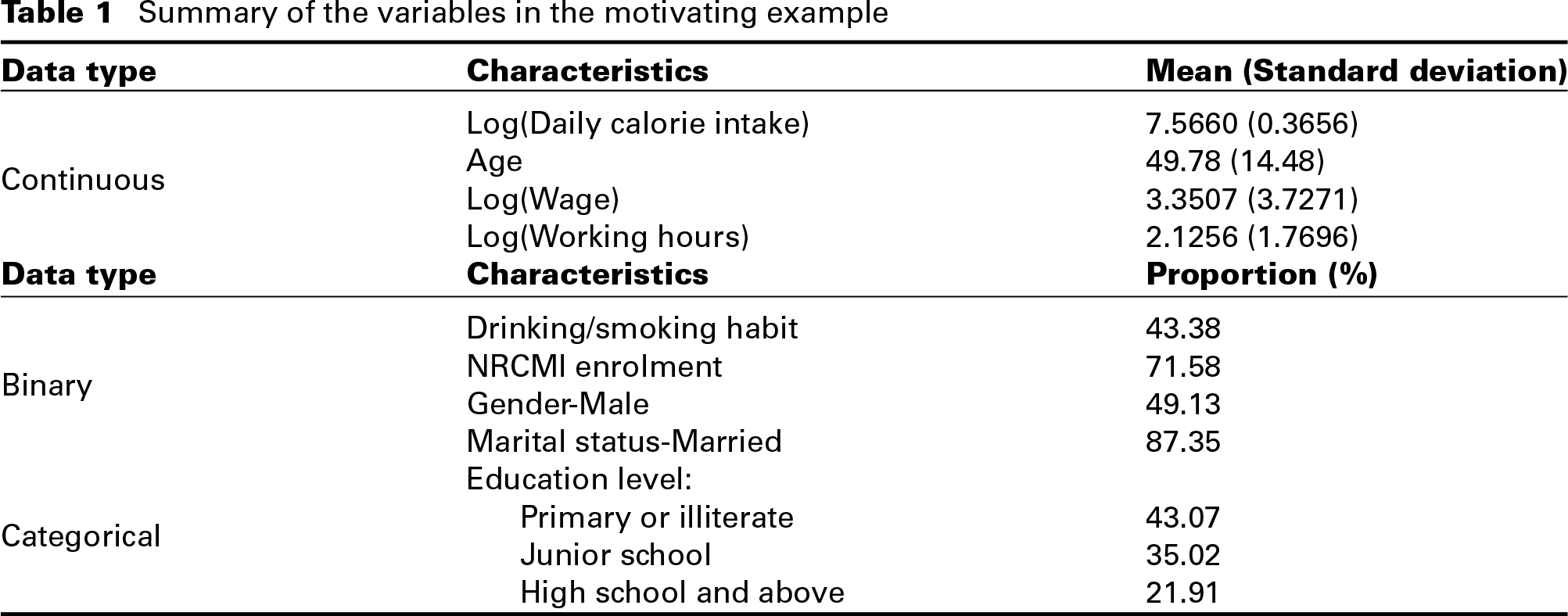
In this article, we try to explore the effects of NRCMI insurance on health style of the respondents. Two variables, drinking or smoking habit and daily calorie intake, are selected as the two outcomes for reflecting the health style of a person. Drinking or smoking habit is a dummy variable representing whether the individual has a habit of drinking or smoking, while daily calorie intake is a continuous variable reflecting the amount of calorie intake per day. The key explanatory variable in our analysis is a dummy variable indicating whether a respondent has enroled in the NRCMI insurance in the survey year. Other social-demographic characteristics include age, gender, marital status, education level and wage. Age is recorded in years; gender is categorized as male and female; marital status is divided into married and single (including never married, divorced, widowed and separated); education level is classified into three levels including primary or illiterate, junior school and high school and above and wage is a continuous variable indicating the economic condition of an individual, which suffers from missing values. The missing percentage is up to 42.51%, leading to 3 075 missing responds among a total number of 7 234 individuals. In order to model this missing covariate, another variable working hour is considered. A summary of these variables are given in Table 1.

Table 1:

Summary of the variables in the motivating example

Data type	Characteristics	Mean (Standard deviation)
Continuous	Log(Daily calorie intake)	7.5660 (0.3656)
		Age	49.78 (14.48)
		Log(Wage)	3.3507 (3.7271)
		Log(Working hours)	2.1256 (1.7696)
Data type	Characteristics	Proportion (%)
Binary	Drinking/smoking habit	43.38
	NRCMI enrolment	71.58
	Gender-Male	49.13
	Marital status-Married	87.35
Categorical	Education level:
	Primary or illiterate	43.07
	Junior school	35.02
	High school and above	21.91

In this motivating example, the two responses, drinking or smoking habit and daily calorie intake, are in the form of mixed data types. By applying a Kruskal–Wallis test for these two responses, it is shown that these two responses are related to each other with a test statistics value of 269.90 at a significance level of 0.05. As a result, we cannot simply ignore the dependence between these two outcomes and apply a separate analysis. Instead, a joint analysis is preferred in order to consider the relationship between them. In addition, there are missing values in one of the covariates in this dataset, which would lead to lower power if simply applying a CC analysis. Moreover, when the missing data mechanism is not missing completely at random (MCAR), the CC approach would lead to biased estimates. Therefore, models should be built for the missing covariate and even for the missing data mechanism.

3 The proposed model

3.1 Complete data model

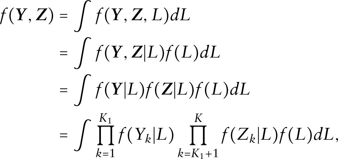
Consider a dataset with $N$ subjects and $K$ outcome variables, such that the first $K_{1}$ outcome variables are binary while the remaining $K - K_{1}$ outcome variables are continuous. For $i = 1, \dots, N$ , the binary and continuous measurements of the $i$ th subject for variable $k$ are denoted by $Y_{ki} (k = 1, \dots, K_{1})$ and $Z_{ki} (k = K_{1} + 1, \dots, K)$ , respectively. The vector of mixed binary and continuous outcome variables can be denoted by ${Y = (Y_{1}, \dots, Y_{K_{1}})^{'}, Z = (Z_{K_{1} + 1}, \dots, Z_{K})^{'}}$ , where $Y_{k} = (Y_{k 1}, \dots, Y_{kN})^{'}$ and $Z_{k} = (Z_{k 1}, \dots, Z_{kN})^{'}$ . Considering the dependence among these mixed responses, the LVM is employed for joint analysis.

Suppose $L$ denotes the shared latent variable in the LVM. Based on the assumption that all the mixed outcomes are conditionally independent given this latent variable, the joint distribution in the LVM can be given as

\begin{matrix} f (Y, Z) & = \int f (Y, Z, L) dL \\ = \int f (Y, Z | L) f (L) dL \\ = \int f (Y | L) f (Z | L) f (L) dL \\ = \int \prod_{k = 1}^{K_{1}} f (Y_{k} | L) \prod_{k = K_{1} + 1}^{K} f (Z_{k} | L) f (L) dL, \end{matrix}

where $f (Y_{k} | L)$ and $f (Z_{k} | L)$ are the conditional distributions of $Y_{k}$ and $Z_{k}$ given $L$ , respectively. For the conditional distribution of the binary outcome, a Bernoulli distribution can be assigned as, for $k = 1, \dots, K_{1}$ ,

Y_{k} | L, X^{*} ~ Bernoulli (μ_{y k}), logit (μ_{y k}) = β_{y 0 k} + β_{y k} X^{*} + L,

3.1

where $β_{y 0 k}$ is the intercept, and $β_{yk}$ is the coefficient vector corresponding to the $p$ -dimensional covariate vector $X^{*}$ .

Similarly, we assume a normal conditional distribution for the continuous outcome, which is given by, for $k = K_{1} + 1, \dots, K$ :

Z_{k} | L, X^{*} ~ N (μ_{z} k, τ_{z} {_{k}}^{-}^{1}), μ_{z}_{k} = β_{z}_{k} X^{*} + L,

3.2

where $τ_{zk}$ represents the precision parameter for variable $Z_{k}$ . The intercept here is restricted to be 0 for identification, and $β_{zk}$ represents the coefficient vector.

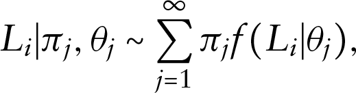
For the latent variable $L$ , a DP mixtures prior is assigned. Suppose the unknown distribution for the random samples of the latent variable $L_{i} (i = 1, \dots, N)$ is denoted by $F$ . A DP mixtures prior on $F$ is denoted by

\begin{matrix} L_{i} \sim F (L_{i}) = \int f (L_{i} | θ) G (d θ), G \sim DP (κ, G_{0}), \end{matrix}

where $f (L_{i} | θ)$ is the kernel of the DP mixtures prior, which is indexed by a finite dimensional parameter $θ$ . Similar to the DP prior, the DP mixtures prior can also be represented through the stick-breaking construction (Sethuraman, 1994). Therefore, we have

\begin{matrix} L_{i} | π_{j}, θ_{j} \sim \sum_{j = 1}^{\infty} π_{j} f (L_{i} | θ_{j}), \end{matrix}

where $θ_{j} \sim G_{0}, π_{j} = V_{j} \prod_{k < j} (1 - V_{k})$ and $V_{j} \sim Beta (1, κ)$ .

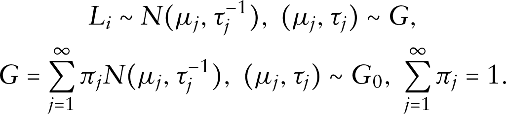
DP mixtures are countable mixtures with an infinite number of components and specific priors on the weights $π_{j}$ and the component-specific parameters $θ_{j}$ . The DP mixtures prior can support on a large class of distributions depending on appropriate choices of the kernel $f (L_{i} | θ)$ (Barrientos et al., 2012; Rodriguez and Müller, 2013). For a DP mixture of normals, we have

L_{i} | G ~ \int N (L_{i} | μ_{j}, τ_{j}^{-}^{1}) G (d μ_{j}, d τ_{j}), G ~ D P (κ, G_{0}),

which is equivalent to

\begin{matrix} L_{i} \sim N (μ_{j}, τ_{j}^{- 1}), (μ_{j}, τ_{j}) \sim G, \\ G = \sum_{j = 1}^{\infty} π_{j} N (μ_{j}, τ_{j}^{- 1}), (μ_{j}, τ_{j}) \sim G_{0}, \sum_{j = 1}^{\infty} π_{j} = 1 . \end{matrix}

The DP mixture of normals prior allows a flexible continuous distribution for the latent variable.

According to models (3.1)–(3.3), when observing complete data $D = {Y, Z, X^{*}}$ , the likelihood of the unknown parameters $Θ = (β_{y 0 k}, β_{yk}, β_{zk}, τ_{zk}, L)$ can be obtained as

\begin{matrix} L & (Θ | D) = \prod_{i = 1}^{N} f (Y_{i}, Z_{i} | X_{i}^{*}) \\ = \prod_{i = 1}^{N} \int \prod_{k = 1}^{K_{1}} f (Y_{ki} | L_{i}, X_{i}^{*}, β_{y 0 k}, β_{yk}) \prod_{k = K_{1} + 1}^{K} f (Z_{ki} | L_{i}, X_{i}^{*}, β_{zk}, τ_{zk}) f (L_{i}) {dL}_{i}, \end{matrix}

where $f (Y_{ki} | L_{i}, X_{i}^{*}, β_{y 0 k}, β_{yk})$ and $f (Z_{ki} | L_{i}, X_{i}, β_{zk}, τ_{zk})$ are given in (3.1) and (3.2), respectively.

3.2 Incomplete data model

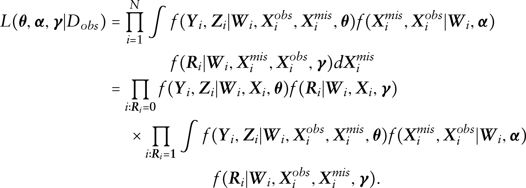
In some situations such as our motivating example, missing values may occur in some of the covariates. In such cases, a selection model within the Bayesian framework can be applied to accommodate missing data situations. For the $p$ -dimensional covariates $X^{*}$ , suppose that the first $q (q \leq p)$ covariates have missing values while the remaining $(p - q)$ covariates are completely observed, which are denoted by $X$ and $W$ , respectively. Then we have $X^{*} = (X, W)$ , where $X = (X_{1}, \dots, X_{q})^{'}$ is the covariates subjected to missingness, and $W = (W_{1}, \dots, W_{p - q})^{'}$ refers to the fully observed covariates. The corresponding $q$ -dimensional missing indicators can be denoted by $R = (R_{1}, \dots, R_{q})^{'}$ , where for $k = 1, \dots, q$ , $R_{k} = (R_{k 1}, \dots, R_{kN})^{'}$ with $R_{ki} = 1$ if $X_{ki}$ is missing and $R_{ki} = 0$ if $X_{ki}$ is observed. Furthermore, let $X^{obs}$ refer to the components of $X$ that are observed and $X^{mis}$ refer to the components of $X$ that are missing. Suppose that $D_{obs} = (Y, Z, W, X^{obs}, R)$ denotes the observed data. The incomplete data likelihood can be obtained by integrating out the missing components $X^{mis}$ , which is given by

\begin{matrix} L (Θ | D_{obs}) = \int f (Y, Z, X, R | W) d X^{mis}, \end{matrix}

(3.4)

where $f (Y, Z, X, R | W)$ denotes the joint distribution of the observed data, missing covariates and missingness probabilities, which, in selection model framework, is given as

f (Y, Z, X, R | W) = f (Y, Z | X, W) f (X | W) f (R | X, W),

(3.5)

where $f (X | W)$ and $f (R | X, W)$ represent the distributions of the missing covariates and missing indicators, respectively.

3.2.1 Model for the missing covariates

In the joint distribution (3.5), it is crucial to specify a model $f (X | W)$ for the missing covariates. Following Lipsitz and Ibrahim (1996) and Ibrahim et al. (1999), the missing covariates distribution can be specified through a series of one-dimensional conditional distributions given by

\begin{matrix} f (X_{1}, \dots, X_{q} | W, α) & = f (X_{q} | X_{1}, \dots, X_{q - 1}, W, α_{q}) \\ \times f (X_{q - 1} | X_{1}, \dots, X_{q - 2}, W, α_{q - 1}) \dots f (X_{1} | W, α_{1}), \end{matrix}

(3.6)

where $α_{k} (k = 1, \dots, q)$ is the indexing parameter vector for the $k$ th conditional distribution, and $α = (α_{1}, \dots, α_{q})^{'}$ . Here, we assume that $α_{1}, \dots, α_{q}$ are distinct.

There are many choices for defining (3.6), and Chen and Ibrahim (2001) gave some guidelines for specifying this distribution. For missing categorical covariates, logistic, probit or complementary log-log links are suitable for the conditional missing covariate distribution. Ordinal regression models can be applied for the missing ordinal covariates, while Poisson regression can be used for count variables. Both normal, log-normal and exponential distributions can be built for the continuous covariates.

In our motivating example, there is only one continuous missing covariate Wage, thus the missing covariate distribution can be simplified as $f (X_{1} | W, α)$ , and a normal distribution can be built as $X_{1} \sim N (μ_{x}, τ_{x}^{- 1})$ , where $μ_{x}$ is the mean function and $τ_{x}$ is the precision parameter.

3.2.2 Model for the missing data mechanism

Similar to the missing covariates distribution, the model for the missing data mechanism can also be written as the form of a product of one-dimensional conditional distributions as (3.6), which is given by

\begin{matrix} f (R_{1}, \dots, R_{q} & | X, W, ϕ) = f (R_{q} | R_{1}, \dots, R_{q - 1}, X, W, ϕ_{q}) \\ \times f (R_{q - 1} | R_{1}, \dots, R_{q - 2}, X, W, ϕ_{q - 1}) \dots f (R_{1} | X, W, ϕ_{1}), \end{matrix}

(3.7)

where $ϕ = (ϕ_{1}, \dots, ϕ_{q})^{'}$ parameterizes the missing data mechanism model with $ϕ_{k} (k = 1, \dots, q)$ as a vector of indexing parameters for the $k$ th conditional distribution. For these one-dimensional conditional distributions for the binary missing indicators, a logistic or probit regression model can be built.

According to Rubin (1976), there are three types of missing data mechanisms, including MCAR, missing at random (MAR), and missing not at random (MNAR). Under some conditions, MCAR and MAR are categorized as ignorable missingness since the missingness does not depend on the missing variables, while MNAR is regarded as non-ignorable.

In our motivating example, the model for the missing data mechanism can be simplified as $f (R_{1} | X, W, ϕ)$ since there is only one covariate that suffers from missing. A logit regression model can be assumed for $R_{1}$ . For the missing covariate Wage, it is more likely to be missing if it is of high or low levels (Mason et al., 2010). Therefore, we assume that the missing data mechanism of this covariate is non-ignorable, meaning that the missingness depends on the missing covariate itself.

4 Bayesian inference and model comparison

4.1 Bayesian inference

Within the Bayesian framework, posterior estimates of the parameters can be obtained from their corresponding posterior distributions through Markov chain Monte Carlo (MCMC) algorithms. Suppose $Θ = (β_{y 0 k}, β_{yk}, β_{zk}, τ_{zk}, α, τ_{x}, ϕ$ , $κ, μ_{j}, τ_{j})$ is the vector of parameters, where $κ$ , $μ_{j}$ and $τ_{j}$ are the parameters corresponding to the DP mixture of normals prior on the latent variable. The joint posterior distribution is given by

\begin{matrix} π (Θ | D_{obs}) L (Θ | D_{obs}) π (Θ), \end{matrix}

where $L (Θ | D_{obs})$ is the incomplete data likelihood given in (3.1) and $π (Θ)$ is the joint prior distribution of the parameters. Generally, we assume that the priors of the parameters are independent a prior. In this article, the following priors are assigned: $β_{y 0 k} \sim N (0, ψ_{β 0}^{- 1})$ , $β_{yk} \sim N (0, ψ_{β y}^{- 1})$ , $β_{zk} \sim N (0, ψ_{β z}^{- 1})$ , $τ_{zk} \sim Gamma (0.001, 0.001)$ , $α_{k} \sim N (0, ψ_{α k}^{- 1})$ , $ϕ_{k} \sim N (0, ψ_{ϕ k}^{- 1})$ , $τ_{zk} \sim Gamma (1, 1)$ , $τ_{x} \sim Gamma (0.001, 0.001)$ , $κ \sim Gamma (1, 1)$ , $μ_{j} \sim N (0, 1)$ and $τ_{j} \sim Gamma (1, 1)$ . Note that $ψ_{β 0}$ , $ψ_{β y}$ , $ψ_{β z}$ , $ψ_{α k}$ and $ψ_{ϕ k}$ are pre-specified hyperparameters. In this article, we use $ψ_{β 0} = ψ_{ϕ k} = 1$ and $ψ_{β y} = ψ_{β z} = ψ_{α k} = 0.001$ .

Usually, the posterior distributions of the parameters cannot be obtained easily due to high-dimensional integrals. MCMC algorithms provide an alternative to sample from the posterior distributions. It requires sampling the following parameters in turn from their respective full conditional distributions. Several existing packages and software facilitate the implementation of the MCMC algorithms, such as WinBUGS (Spiegelhalter et al., 2003), JAGS (Hornik et al., 2003), Stan (Stan Development Team, 2019) and nimble (de Valpine et al., 2017). nimble is a relatively new and powerful R package for programming with BUGS models using syntax similar to WinBUGS and JAGS, but with more flexibility in defining the models and algorithms. Users can interface with R, and nimble will generate C++ code for faster computation (Ma and Chen, 2019). In this article, we use nimble for implementing the MCMC sampling algorithms for posterior inference.

4.2 Model comparison

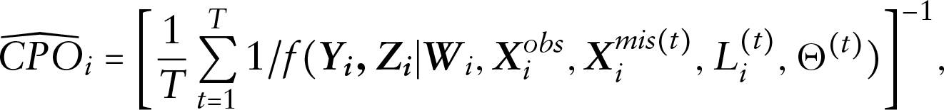
Model comparison is an important topic in statistical modelling since the actual model, and the missing data mechanism are unknown. For our model, we mainly focus on selecting (a) different priors for the latent variable $L$ and (b) different models for the missing data mechanism. For (a), we employ the logarithm of the pseudo-marginal likelihood (LPML) for model comparison. LPML can be calculated via the conditional predictive ordinates (CPOs Geisser, 1993). Let $D_{obs}^{(- i)}$ denote the observed dataset $D_{obs}$ with the $i$ th observation deleted. The CPO statistic in our model with non-ignorable missing covariates can be defined as

\begin{matrix} {CPO}_{i} = \int f (Y_{i}, Z_{i} & | W_{i}, X_{i}^{mis}, X_{i}^{obs}, L_{i}) f (L_{i}) \\ f (X_{i}^{mis}, X_{i}^{obs} | W_{i}) π (Θ | D_{obs}^{(- i)}) d X_{i}^{mis} {dL}_{i} d Θ, \end{matrix}

where $π (Θ | D_{obs}^{(- i)})$ is the posterior density of $Θ$ given $D_{obs}^{(- i)}$ . In practice, a Monte Carlo estimate of the CPO can be obtained from MCMC samples of the posterior distributions. Suppose ${(Θ^{(t)}, X_{i}^{mis (t)}, L_{i}^{(t)}) : t = 1, \dots, T}$ are the observations simulated from the conditional distribution $f (X_{i}^{mis}, L_{i}, Θ | Y_{i},$ $Z_{i}, X_{i}^{obs}, W_{i})$ via MCMC algorithms at the $t$ th iteration, then the Monte Carlo estimate of CPO is given by

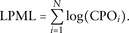
\begin{matrix} {\hat{CPO}}_{i} = [\frac{1}{T} \sum_{t = 1}^{T} 1 / f (Y_{i}, Z_{i} | W_{i}, X_{i}^{obs}, X_{i}^{mis (t)}, L_{i}^{(t)}, Θ^{(t)})]^{- 1}, \end{matrix}

and LPML can be given as

\begin{matrix} LPML = \sum_{i = 1}^{N} \log ({CPO}_{i}) . \end{matrix}

A larger value of LPML means a better fit of the model.

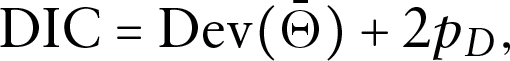
For (b), since the main objective is to assess the fit of the model for the missing data mechanism model, here we use the conditional version of deviance information criterion (DIC; Spiegelhalter et al., 2002), ${DIC}^{R}$ , to select the missing data mechanism model. The DIC is defined as

\begin{matrix} DIC = Dev (\overset{̅}{Θ}) + 2 p_{D}, \end{matrix}

where $Dev (\overset{̅}{Θ})$ is the deviance function, $p_{D} = \overset{̅}{Dev} (Θ) - Dev (\overset{̅}{Θ})$ is the effective number of model parameters, $\overset{̅}{Θ}$ is the posterior mean of the parameters and $\overset{̅}{Dev} (Θ)$ is the posterior mean of $Dev (Θ)$ . For ${DIC}^{R}$ , the deviance function is defined using the missing data mechanism model only, which is $Dev (\overset{̅}{Θ}) = - 2 \log f (R_{1}, \dots, R_{q} | X, W, ϕ)$ . A smaller ${DIC}^{R}$ value represents that the missing data mechanism model is more preferred.

5 ISNI in latent variable model with missing covariates

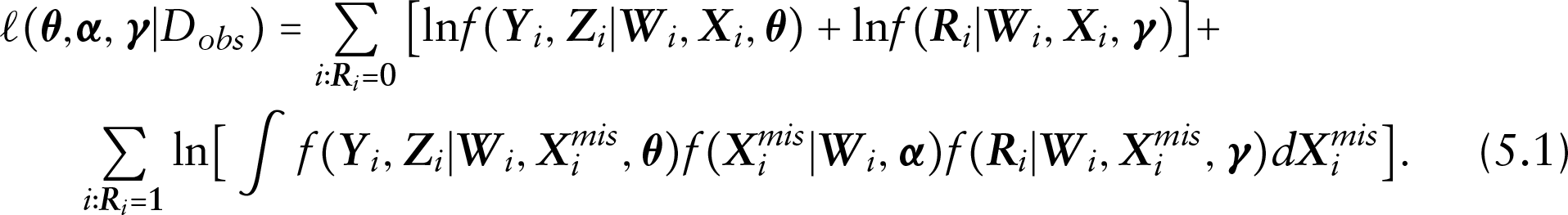
In this section, we extend the Bayesian ISNI to the proposed LVM with missing covariates. The response model $f (Y_{i}, Z_{i} | W_{i}, X_{i}, θ)$ is specified via the LVM, the missing covariate model is $f (X_{i} | W_{i}, α)$ and the model for the missing data mechanism can be rewritten as $f (R_{i} | W_{i}, X_{i}, γ) = h (γ_{0}^{T} W_{i} + γ_{1}^{T} X_{i})$ . With this model, the missing data mechanism is ignorable if $γ_{1} = 0$ and the parameter of interest is distinct from $γ = (γ_{0}, γ_{1})$ . Given these distributions, the incomplete data likelihood can be written as

\begin{matrix} L (θ, α, γ | D_{obs}) & = \prod_{i = 1}^{N} \int f (Y_{i}, Z_{i} | W_{i}, X_{i}^{obs}, X_{i}^{mis}, θ) f (X_{i}^{mis}, X_{i}^{obs} | W_{i}, α) \\ f (R_{i} | W_{i}, X_{i}^{mis}, X_{i}^{obs}, γ) d X_{i}^{mis} \\ = \prod_{i : R_{i} = 0} f (Y_{i}, Z_{i} | W_{i}, X_{i}, θ) f (R_{i} | W_{i}, X_{i}, γ) \\ \times \prod_{i : R_{i} = 1} \int f (Y_{i}, Z_{i} | W_{i}, X_{i}^{obs}, X_{i}^{mis}, θ) f (X_{i}^{mis}, X_{i}^{obs} | W_{i}, α) \\ f (R_{i} | W_{i}, X_{i}^{obs}, X_{i}^{mis}, γ) . \end{matrix}

The corresponding log-likelihood is denoted by

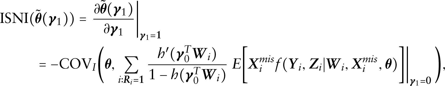
\begin{matrix} ℓ (θ, & α, γ | D_{obs}) = \sum_{i : R_{i} = 0} [\ln f (Y_{i}, Z_{i} | W_{i}, X_{i}, θ) + \ln f (R_{i} | W_{i}, X_{i}, γ)] + \\ \sum_{i : R_{i} = 1} \ln [\int f (Y_{i}, Z_{i} | W_{i}, X_{i}^{mis}, θ) f (X_{i}^{mis} | W_{i}, α) f (R_{i} | W_{i}, X_{i}^{mis}, γ) d X_{i}^{mis}] . \end{matrix}

(5.1)

According to Xie (2009), the ISNI can be defined as

\begin{matrix} ISNI ( & \tilde{θ} (γ_{1})) = {\frac{\partial \tilde{θ} (γ_{1})}{\partial γ_{1}}|}_{γ_{1} = 1} \\ = - {COV}_{I} (θ, \sum_{i : R_{i} = 1} \frac{h^{'} (γ_{0}^{T} W_{i})}{1 - h (γ_{0}^{T} W_{i})} {E [X_{i}^{mis} f (Y_{i}, Z_{i} | W_{i}, X_{i}^{mis}, θ)]|}_{γ_{1} = 0}), \end{matrix}

where $E [X_{i}^{mis} f (Y_{i}, Z_{i} | W_{i}, X_{i}^{mis}, θ)]$ is a mean function and ${COV}_{I} (\cdot)$ denotes the posterior covariance under the ignorable model.

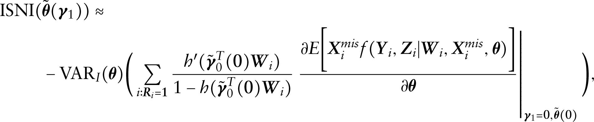
Alternatively, the ISNI can be approximated as

\begin{matrix} ISNI ( & \tilde{θ} (γ_{1})) \\ - {VAR}_{I} (θ) (\sum_{i : R_{i} = 1} \frac{h^{'} ({\tilde{γ}}_{0}^{T} (0) W_{i})}{1 - h ({\tilde{γ}}_{0}^{T} (0) W_{i})} {\frac{\partial E [X_{i}^{mis} f (Y_{i}, Z_{i} | W_{i}, X_{i}^{mis}, θ)]}{\partial θ}|}_{γ_{1} = 0, \tilde{θ} (0)}), \end{matrix}

where ${VAR}_{I} (θ)$ is the posterior variance-covariance matrix of $θ$ under the ignorable model, and ${\tilde{γ}}_{0}^{T} (0)$ and $\tilde{θ} (0)$ represent the posterior means of $θ$ and $γ_{0}$ under the ignorable model, respectively. With MCMC sampling iterations, ISNI of each parameter of interest can be obtained.

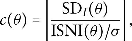
When the response is continuous, the value of ISNI depends on the scale of the continuous response. In order to compare the sensitivity of $γ_{1}$ on different parameters, a transformation can be made as

\begin{matrix} c (θ) = |\frac{{SD}_{I} (θ)}{ISNI (θ) / σ}|, \end{matrix}

where ${SD}_{I} (θ)$ is the posterior standard deviation of the parameter $θ$ under the ignorable model, $σ$ is the standard deviation of the continuous response. A small $c (θ)$ value means large local sensitivity (Xie, 2009).

6 Simulation study

In this section, a simulation study is conducted to verify the performance of the model comparison criteria and the proposed methodology. $S = 100$ datasets were simulated with $N = 100$ observations in each dataset. In each replication, the latent variable $L$ was generated from a mixture of two normal distributions $0.5 N (- 2, 1) + 0.5 N (2, 1)$ , leading $L$ to be a bimodal variable. Covariates $X = (X_{1}, W_{1}, W_{2})$ were generated with $W_{1}$ and $W_{2}$ following standard normal distributions. $X_{1}$ was generated from $N (α_{0} + α_{1} W_{1} + α_{2} W_{2}, τ_{x}^{- 1})$ with $α_{0} = - 1$ , $α_{1} = - 1$ , $α_{2} = 2$ and $τ_{x} = 1$ . We assumed that $K_{1} = 1$ and $K = 2$ , meaning that two mixed responses were generated, one of which was a binary response $Y$ , and the other was a continuous response $Z$ . We assumed that $μ_{y} = 1 + X_{1} + W_{1} + L$ , $μ_{z} = 3 X_{1} - W_{1} + L$ and $τ_{z} = 1$ . Missing data for $X_{1}$ were generated with a non-ignorable missing data mechanism. Specifically, let $R_{i} = 1$ if $X_{1 i}$ was missing and $R_{i} = 0$ if $X_{1 i}$ was observed. A logistic regression model was built for the missing indicator $R_{i}$ as

\begin{matrix} f (R_{i} | X_{1 i}, W_{1 i}) = \frac{\exp (ϕ_{0} + ϕ_{1} X_{1 i} + ϕ_{2} W_{1 i})}{1 + \exp (ϕ_{0} + ϕ_{1} X_{1 i} + ϕ_{2} W_{1 i})}, \end{matrix}

where $ϕ_{0} = - 1$ , $ϕ_{1} = 1$ and $ϕ_{2} = - 1$ . The average percentage of missing $X_{1}$ in $S = 100$ simulations in this study is about 28%.

For the binary and continuous responses, model (3.1) and (3.2) are fitted, respectively. For the missing covariate $X_{1}$ , a normal distribution is assumed with mean $(α_{0} + α_{1} W_{1} + α_{2} W_{2})$ and precision $τ_{x}$ . For the missing data mechanism model, we firstly assume a non-ignorable model, which is given by

\begin{matrix} R_{i} \sim Bernoulli ({pR}_{i}), logit ({pR}_{i}) = ϕ_{0} + ϕ_{1} X_{1 i} + ϕ_{2} W_{1 i} + ϕ_{3} W_{2 i} . \end{matrix}

For the performance of LPML, we compare models with different priors on the latent variable $L$ and calculate the percentage that the criteria choosing the correct model. Let $M_{true}$ denote the true model where $L$ follows a mixture normal distribution $0.5 N (- 2, 1) + 0.5 N (2, 1)$ , $M_{0}$ denote the model with a DP mixture of normals prior for $L$ $M_{1}$ denote the model with a normal prior for $L$ , and $M_{2}$ denote the model with a $t_{1}$ -distributed prior for $L$ . The average values of LPML under these three models are shown in Table 2.

Table 2:

The average of the LPML values of the competitive models with different priors on $L$

Model	$M_{true}$	$M_{0}$	$M_{1}$	$M_{2}$
LPML	$-$ 251.93	$-$ 258.07	$-$ 262.45	$-$ 286.17

From Table 2, we can see that model $M_{true}$ has the largest LPML value among the competitive models, indicating that LPML can choose the true model in this simulation. $M_{0}$ with a DP mixtures prior on the latent variable is more preferred than the other two models due to a larger LPML value. The percentage that the criteria selecting $M_{0}$ over $M_{1}$ is 71%, and the percentage for selecting $M_{0}$ over $M_{2}$ is 100%. Therefore, under the setting that $L$ actually follows a normal mixture model, besides the true model, the DP mixture of normals prior performs better than normal priors and heavy-tailed priors.

Here, we apply the ${DIC}^{R}$ measure for selecting the model for missing data mechanism. In model $M_{0}$ , we assume an non-ignorable missingness model that the missingness depends on the missing variable itself. We build another model similar to $M_{0}$ except for the model for missing data mechanism, denoting by $M_{3}$ . The missingness model in $M_{3}$ only depends on the observed variables, leading to an ignorable missing data mechanism assumption, that is, $logit ({pR}_{i}) = ϕ_{0}^{'} + ϕ_{1}^{'} W 1^{i} + ϕ_{2}^{'} W_{2 i}$ . The ${DIC}^{R}$ values for models $M_{0}$ and $M_{3}$ are 65.64 and 100.95, respectively. Since $M_{0}$ have a smaller value of ${DIC}^{R}$ , the non-ignorable missingness model is selected over the ignorable one in model $M_{3}$ , which conforms to our simulation setting.

For assessing the precision of the posterior estimates, we employ the following assessment measures. Take parameter $α_{1}$ as an example: $Bias = \frac{1}{S} \sum_{s = 1}^{S} ({\hat{α}}_{1} - α_{1}^{0})$ , $SD = \frac{1}{S} \sum_{s = 1}^{S} sd ({\hat{α}}_{1})$ , $MSE = \frac{1}{S} \sum_{s = 1}^{S} ({\hat{α}}_{1} - α_{1}^{0})^{2}$ and $CP = \frac{1}{S} \sum_{s = 1}^{S} 1 (α_{1}^{0} \in HPD ({\hat{α}}_{1}))$ , where ${\hat{α}}_{1}$ denotes the posterior estimation of $α_{1}$ in the $s$ th iteration, $α_{1}^{0}$ denotes the true value of parameter $α_{1}$ , $sd ({\hat{α}}_{1})$ denotes the posterior standard deviation of the estimate and $HPD ({\hat{α}}_{1})$ denotes the estimated 95% HPD interval of ${\hat{α}}_{1}$ in the $s$ th iteration. The simulation results under the proposed model and the alternative models are shown in Table 3.

Table 3:

Simulation results under the proposed model $M_{0}$ and the separate analysis model

*Parameter	True	The proposed model $M_{0}$				The separate analysis model
*Parameter		value	Bias	SD	MSE	CP	Bias	SD	MSE	CP
$β_{y 0}$	1	$-$ 0.1195	0.3776	0.1178	0.98	$-$ 0.4067	0.2697	0.2353	0.67
$β_{y 1}$	1	$-$ 0.0914	0.2020	0.0454	0.93	$-$ 0.3884	0.1438	0.1682	0.29
$β_{y 2}$	1	$-$ 0.0964	0.4362	0.1805	0.94	$-$ 0.4095	0.2878	0.2622	0.65
$β_{z 1}$	3	0.0180	0.1260	0.0155	0.95	0.0016	0.1077	0.0127	0.92
$β_{z 2}$	$-$ 1	$-$ 0.0226	0.2950	0.0782	0.98	$-$ 0.0395	0.3070	0.0817	0.98
$τ_{z}$	1	0.1257	0.4183	0.1899	0.97	$-$ 0.8222	0.0285	0.6765	0.00
$α_{0}$	$-$ 1	0.0059	0.1135	0.0117	0.93	0.0110	0.1109	0.0121	0.95
$α_{1}$	$-$ 1	0.0017	0.1158	0.0132	0.95	$-$ 0.0009	0.1153	0.0141	0.94
$α_{2}$	2	$-$ 0.0164	0.1143	0.0103	0.98	$-$ 0.0113	0.1125	0.0096	0.98
$τ_{x 1}$	1	0.0321	0.1674	0.0282	0.96	0.0078	0.1633	0.0247	0.95
$ϕ_{0}$	$-$ 1	0.1417	0.3367	0.0987	0.96	0.0711	0.3421	0.0918	0.98
$ϕ_{1}$	1	0.0917	0.2584	0.0936	0.92	0.0921	0.2590	0.0956	0.93
$ϕ_{2}$	$-$ 1	0.1330	0.3772	0.1318	0.97	0.1271	0.3824	0.1291	0.98

From Table 3, we can see that the posterior estimates have relatively small bias and MSE, and the CPs of the estimates are both larger than 0.92, indicating that the posterior estimation procedure has good performance under our simulation setting.

We also carry out the separate analysis to explore the difference between joint analysis and separate analysis. For separate analysis, we build the model without the latent variable $L$ in (3.1) and (3.2). By excluding $L$ , the dependence between these two responses is no longer considered and independence is assumed instead. The LPML value for the separate analysis model is $-$ 302.33, and by comparing it with the LPML value of model $M_{0}$ in Table 2, we can say that the model comparison criteria chooses the joint analysis model as the better model. The posterior estimates under the separate analysis model are shown in Table 3 as well. From Table 3, we can see that generally, under the separate analysis model, the bias and MSE of the posterior estimates of parameters in the response model, especially in the binary response model, are greatly larger than those under the joint analysis model. Besides, the corresponding CPs are smaller than 0.70, indicating that separate analysis is not good enough under our simulation setting.

We also carry out a CC analysis to explore the impact of ignoring the missingness on the posterior estimates. In each replication, the missing records are excluded and model (3.1) and (3.2) are fitted. The simulation results of the CC analysis are given in Table 4. By comparing the results in Table 4 with those under model $M_{0}$ , we can see that the bias and MSE of the posterior estimates under CC analysis are larger than those under the proposed model, indicating that simply excluding the missing records may lead to more biased estimates when the missing data mechanism is not MCAR.

Table 4:

Simulation results under CC analysis

*Parameter	True	CC analysis
*Parameter		value	Bias	SD	MSE	CP
$β_{y 0}$	1	$-$ 0.2382	0.4825	0.2056	0.89
$β_{y 1}$	1	$-$ 0.1318	0.2507	0.0783	0.91
$β_{y 2}$	1	$-$ 0.1827	0.5231	0.3005	0.92
$β_{z 1}$	3	0.0229	0.1389	0.0198	0.95
$β_{z 2}$	$-$ 1	$-$ 0.0563	0.3174	0.0953	0.98
$τ_{z}$	1	0.1679	0.6283	0.2549	0.97
$α_{0}$	$-$ 1	$-$ 0.1877	0.1296	0.0523	0.65
$α_{1}$	$-$ 1	0.1232	0.1329	0.0315	0.86
$α_{2}$	2	$-$ 0.1325	0.1323	0.0360	0.83
$τ_{x 1}$	1	0.1159	0.1872	0.0633	0.91

7 Application in CHNS data

In this section, the proposed methodology is applied to analyse the data introduced in Section 2. The binary response variable is drinking or smoking habit ( $Y$ ), and the continuous response variable is daily calorie intake ( $Z$ ). The covariates used for predicting these two responses include NRCMI enrolment ( $W_{1}$ ), Age ( $W_{2}$ ), Gender ( $W_{3}$ ), Marital status ( $W_{4}$ ), Education level (Junior schools ( $W_{5}$ ), High school and above ( $W_{6}$ )) and Wage ( $X_{1}$ ), where Wage suffers from missingness. Model (3.1)–(3.2) are built as

\begin{matrix} Y | L \sim Bernoulli (μ_{y}), Z | L \sim N (μ_{z}, τ_{z}^{- 1}), \\ logit (μ_{y}) = β_{y 0} + β_{y 1} W_{1} + β_{y 2} W_{2} + β_{y 3} W_{3} + β_{y 4} W_{4} + β_{y 5} W_{5} + β_{y 6} W_{6} + β_{y 7} X_{1} + L; \\ μ_{z} = β_{z 1} W_{1} + β_{z 2} W_{2} + β_{z 3} W_{3} + β_{z 4} W_{4} + β_{z 5} W_{5} + β_{z 6} W_{6} + β_{z 7} X_{1} + L, \end{matrix}

where the latent variable $L$ follows a DP mixture of normals prior described in (3.3). For the missing covariate $X_{1}$ , a normal linear model is assigned as

\begin{matrix} X_{1} \sim N (μ_{x}, τ_{x}^{- 1}), \\ μ_{x} = α_{0} + α_{1} W_{2} + α_{2} W_{3} + α_{3} W_{5} + α_{4} W_{6} + α_{5} W_{7}, \end{matrix}

where $W_{7}$ refers to the Working hour. The missing data mechanism model for the missing indicator is given as

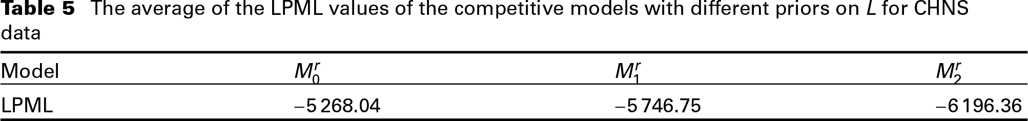
\begin{matrix} \begin{array}{l} R ~ Bernoulli (μ_{r}), \\ logit (μ_{r}) = γ_{00} + γ_{01} W_{1} + γ_{0}_{2} W_{2} + γ_{0}_{3} W_{3} + γ_{0}_{4} W_{4} + γ_{0}_{5} W_{5} + γ_{0}_{6} W_{6} + γ_{1} X_{1} . \end{array} \end{matrix}

7.1

For Bayesian implementation, priors on the unknown parameters are given as described before. R and nimble are used for programming, and a single Markov chain is used with 4 500 samples for posterior estimation after a burn-in of 500 samples. The thinning interval is set to be 10. We assume different priors for $L$ and apply LPML for model selection. The proposed model with a DP mixture of normals prior on $L$ is denoted by $M_{0}^{r}$ , the model with a normal prior is denoted by $M_{1}^{r}$ and the model with a $t$ -distributed prior is denoted by $M_{2}^{r}$ . The LPML results for these competitive models are shown in Table 5.

Table 5:

The average of the LPML values of the competitive models with different priors on $L$ for CHNS data

Model	$M_{0}^{r}$	$M_{1}^{r}$	$M_{2}^{r}$
LPML	$-$ 5 268.04	$-$ 5 746.75	$-$ 6 196.36

From Table 5, we can see that the model with a DP mixture of normals prior on $L$ is more preferred than the other two models since the LPML value of model $M_{0}^{r}$ is the largest. The ${DIC}^{R}$ measure is used for selecting from the non-ignorable and ignorable missing data mechanism models. The model (7.1) used in model $M_{0}^{r}$ represents an non-ignorable missingness model since the missingness depends on the missing covariate $X_{1}$ . The corresponding ${DIC}^{R}$ value is 7 190.66. Let $M_{3}^{r}$ denote the LVM model with ignorable missingness model, which is (7.1) without the last term $γ_{1} X_{1}$ , and the ${DIC}^{R}$ value is 8 110.50. By comparing these two values, we can see that the non-ignorable missingness model is preferred over the ignorable one for the CHNS data.

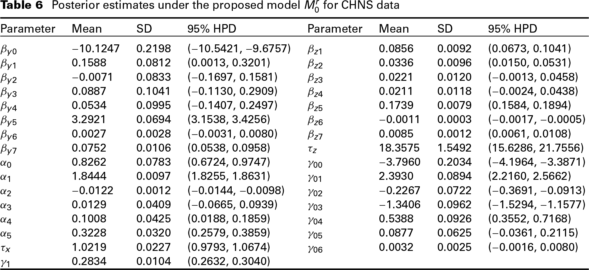
The posterior means, posterior standard deviations and posterior 95% HPD interval of the parameters under model $M_{0}^{r}$ are given in Table 6. From Table 6, we can see that for the binary response model, coefficients $β_{y 1}$ , $β_{y 5}$ and $β_{y 7}$ are significantly larger than 0, meaning that NRCMI enrolment, Junior schools education level and the missing variable Wage have significant positive impact on the drinking or smoking habit. For the continuous response, coefficients $β_{z 1}$ , $β_{z 2}$ , $β_{z 5}$ , $β_{z 6}$ and $β_{z 7}$ are significantly different from 0, meaning that NRCMI enrolment, Age, Junior schools education level and Wage have positive impact on daily calorie intake, while High school and above education level has negative impact on daily calorie intake. We can see that NRCMI insurance enrolment has impact on health style of the respondents. The probability of having drinking or smoking habit and the amount of daily calorie intake are larger for the respondents who enrol in the NRCMI insurance than those who do not enrol in the NRCMI insurance.

Table 6:

Posterior estimates under the proposed model $M_{0}^{r}$ for CHNS data

Parameter	Mean	SD	95% HPD	Parameter	Mean	SD	95% HPD
$β_{y 0}$	$-$ 10.1247	0.2198	( $-$ 10.5421, $-$ 9.6757)	$β_{z 1}$	0.0856	0.0092	(0.0673, 0.1041)
$β_{y 1}$	0.1588	0.0812	(0.0013, 0.3201)	$β_{z 2}$	0.0336	0.0096	(0.0150, 0.0531)
$β_{y 2}$	$-$ 0.0071	0.0833	( $-$ 0.1697, 0.1581)	$β_{z 3}$	0.0221	0.0120	( $-$ 0.0013, 0.0458)
$β_{y 3}$	0.0887	0.1041	( $-$ 0.1130, 0.2909)	$β_{z 4}$	0.0211	0.0118	( $-$ 0.0024, 0.0438)
$β_{y 4}$	0.0534	0.0995	( $-$ 0.1407, 0.2497)	$β_{z 5}$	0.1739	0.0079	(0.1584, 0.1894)
$β_{y 5}$	3.2921	0.0694	(3.1538, 3.4256)	$β_{z 6}$	$-$ 0.0011	0.0003	( $-$ 0.0017, $-$ 0.0005)
$β_{y 6}$	0.0027	0.0028	( $-$ 0.0031, 0.0080)	$β_{z 7}$	0.0085	0.0012	(0.0061, 0.0108)
$β_{y 7}$	0.0752	0.0106	(0.0538, 0.0958)	$τ_{z}$	18.3575	1.5492	(15.6286, 21.7556)
$α_{0}$	0.8262	0.0783	(0.6724, 0.9747)	$γ_{00}$	$-$ 3.7960	0.2034	( $-$ 4.1964, $-$ 3.3871)
$α_{1}$	1.8444	0.0097	(1.8255, 1.8631)	$γ_{01}$	2.3930	0.0894	(2.2160, 2.5662)
$α_{2}$	$-$ 0.0122	0.0012	( $-$ 0.0144, $-$ 0.0098)	$γ_{02}$	$-$ 0.2267	0.0722	( $-$ 0.3691, $-$ 0.0913)
$α_{3}$	0.0129	0.0409	( $-$ 0.0665, 0.0939)	$γ_{03}$	$-$ 1.3406	0.0962	( $-$ 1.5294, $-$ 1.1577)
$α_{4}$	0.1008	0.0425	(0.0188, 0.1859)	$γ_{04}$	0.5388	0.0926	(0.3552, 0.7168)
$α_{5}$	0.3228	0.0320	(0.2579, 0.3859)	$γ_{05}$	0.0877	0.0625	( $-$ 0.0361, 0.2115)
$τ_{x}$	1.0219	0.0227	(0.9793, 1.0674)	$γ_{06}$	0.0032	0.0025	( $-$ 0.0016, 0.0080)
$γ_{1}$	0.2834	0.0104	(0.2632, 0.3040)

For the missing covariate model, coefficients $α_{2}$ , $α_{4}$ and $α_{5}$ are significant, meaning that Age, High school and above education level, and Working hour can help predict the missing values of Wage. For the missing data mechanism model, coefficients $γ_{01}$ , $γ_{02}$ , $γ_{03}$ and $γ_{04}$ are significant. Therefore, NRCMI enrolment, Age, Gender and Marital status can help explain the missingness. People who enrol in the insurance, younger person, females and the married ones tend to reject to report their wage information.

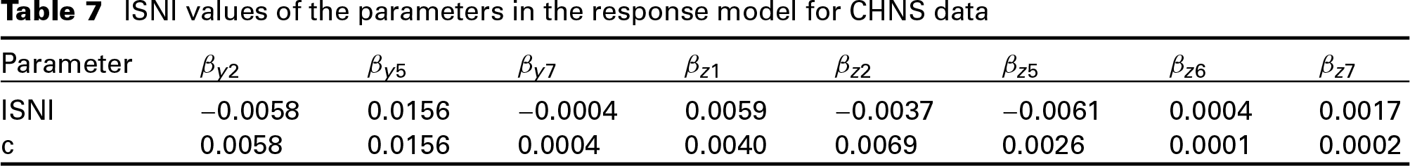
Since the true missing data mechanism is unknown in our study, we carry out a sensitivity analysis using the ISNI index introduced in Section 5 to explore the sensitivity of the parameters on the missingness model. Posterior estimation results in the model with ignorable missing data mechanism, $M_{3}^{r}$ , is used for calculating ISNI values of the parameters. Table 7 shows the ISNI values of the parameters in the response model.

Table 7:

ISNI values of the parameters in the response model for CHNS data

Parameter	$β_{y 2}$	$β_{y 5}$	$β_{y 7}$	$β_{z 1}$	$β_{z 2}$	$β_{z 5}$	$β_{z 6}$	$β_{z 7}$
ISNI	$-$ 0.0058	0.0156	$-$ 0.0004	0.0059	$-$ 0.0037	$-$ 0.0061	0.0004	0.0017
c	0.0058	0.0156	0.0004	0.0040	0.0069	0.0026	0.0001	0.0002

For the parameters in the binary response model, we can see that $β_{y 7}$ has the largest local sensitivity than $β_{y 2}$ and $β_{y 5}$ since it has the smallest $c$ value among these three parameters in Table 7. The local sensitivity of $β_{y 2}$ is larger than that of $β_{y 5}$ . Similarly, in the continuous response model, the local sensitivity of $β_{z 6}$ and $β_{z 7}$ are larger than those of $β_{z 5}$ and $β_{z 2}$ . Through ISNI, we can explore the local sensitivity of the parameters using posterior sampling information under the model with ignorable missing data mechanism. This provides computational convenience than carrying out sensitivity analysis through comparing posterior estimates for a range of the sensitivity parameters.

8 Conclusion

In this article, a semiparametric LVM is built for jointly analysing mixed binary and continuous responses with non-ignorable missing covariate. A DP mixture of normals prior is assigned for the latent variable in the LVM. The LPML measure is used for comparing different priors, and the ${DIC}^{R}$ measure is applied for selecting the missing data mechanism model. An index for measuring the local sensitivity of the parameters, ISNI, is developed to accommodate LVM with non-ignorable missing covariates. The empirical performance of the proposed methodology is examined through a simulation study. And the proposed methodology is applied for the CHNS data to jointly analyse the mixed responses.

Some extensions can be considered for this study. Our proposed methodology is developed for cross-sectional data, which can be extended to longitudinal data structure or other complex data structures. Some other mixed data types, such as ordinal and count variables, can also be considered. In our study, we only take account of missing values in one covariate. More complex situations—including multiple missing covariates, and missing response and covariates—can also be a direction for further research.

Supplementary materials

Supplementary materials for this article, including the code of the model, are available from http://www.statmod.org/smij/archive.html.

Footnotes

Declaration of conflicting interests

Funding

This work was supported by Initial Scientific Research Fund of Young Teachers in Shenzhen University (Grant number 000002110164).

References

Azzalini

Capitanio

(1999) Statistical applications of the multivariate skew normal distribution. Journal of the Royal Statistical Society, Series B (Statistical Methodology) , 61, 579–602.

Baghfalaki

Ganjali

(2011) An EM estimation approach for analyzing bivariate skew normal data with non-monotone missing values. Communications in Sta- tistics: Theory and Methods , 40, 1671–86.

Barrientos

Jara

Quintana

(2012) On the support of MacEachern's dependent Dirichlet processes and extensions. Bayesian Analysis , 7 277–310.

Chen

M-H

Ibrahim

(2001) Maximum likelihood methods for cure rate models with missing covariates. Biometrics , 57, 43–52.

Daniels

Hogan

(2008) Missing Data in Longitudinal Studies: Strategies for Bayesian Modeling and Sensitivity Analysis . Boca Raton: Chapman and Hall/CRC.

De Valpine

Turek

Paciorek

Anderson-Bergman

Lang

Bodik

(2017) Programming with models: Writing statistical algorithms for general model structures with nimble. Journal of Computational and Graphical Statistics , 26, 403–13.

Ganjali

Rezaei

(2005) An influence approach for sensitivity analysis of non- random dropout based on the covariance structure. Iranian Journal of Science and Technology (Sciences) , 29, 287–94.

Geisser

(1993) Predictive Inference: An Introduction . London: Chapman and Hall/CRC.

Görür

Rasmussen

(2010) Dirichlet process Gaussian mixture models: Choice of the base distribution. Journal of Computer Science and Technology , 25, 653–64.

10.

Hornik

Leisch

Zeileis

(2003). Jags: A program for analysis of Bayesian graphical models using Gibbs sampling. In Proceedings of DSC, volume 2, pages 1–1.

11.

Ibrahim

Lipsitz

Chen

M-H

(1999) Missing covariates in generalized linear models when the missing data mechanism is non-ignorable. Journal of the Royal Statistical Society, Series B (Statistical Methodology) , 61, 173–90.

12.

Ibrahim

Chen

M-H

Sinha

(2001) Bayesian Survival Analysis . New York, NY: Springer-Verlag.

13.

Ishwaran

James

(2001) Gibbs sampling methods for stick-breaking priors. Journal of the American Statistical Association , 96, 161–73.

14.

Ishwaran

Zarepour

(2000) Markov chain Monte Carlo in approximate Dirichlet and Beta two-parameter process hierarchical models. Biometrika , 87, 371–90.

15.

Jara

Quintana

Martín

(2008) Linear mixed models with skew-elliptical distributions: A Bayesian approach. Computational Statistics & Data Analysis , 52, 5033–5045.

16.

Lee

S-Y

Xia

Y-M

(2006) Maximum likelihood methods in treating outliers and symmetrically heavy-tailed distributions for nonlinear structural equation models with missing data. Psychometrika , 71, 565–85.

17.

Lin

Chen

(2009) Analysis of multivariate skew normal models with incomplete data. Journal of Multivariate Analysis , 100, 2337–51.

18.

Lipsitz

Ibrahim

(1996) A conditional model for incomplete covariates in para- metric regression models. Biometrika , 83, 916–22.

19.

(1984) On a class of Bayesian nonpara- metric estimates: I. Annals of the Institute of Statistical Mathematics , 12, 351–57.

20.

Troxel

Heitjan

(2005) An index of local sensitivity to nonignorable drop-out in longitudinal modelling. Statistics in Medicine , 24, 2129–50.

21.

Chen

(2019) Bayesian semiparametric latent variable model with DP prior for joint analysis: Implementation with nimble. Statistical Modelling . doi: 10.1177/1471082X18810118

22.

Mason

Best

Richardson

Plewis

(2010) Strategy for modelling non-random missing data mechanisms in observational studies using Bayesian methods. URL http://www.bias-project.org.uk/papers/ StrategySubmitted.pdf (last accessed 22 January 2020).

23.

McCulloch

(2008). Joint modelling of mixed outcome types using latent variables. Statistical Methods in Medical Research , 17, 53–73.

24.

Moustaki

Knott

(2000) Generalized latent trait models. Psychometrika , 65, 391–411.

25.

Müller

Quintana

Jara

Hanson

(2015) Bayesian Nonparametric Data Analysis . New York, NY: Springer.

26.

Murray

Reiter

(2016) Multiple imputation of missing categorical and continuous values via Bayesian mixture models with local dependence. Journal of the American Statistical Association , 111, 1466–79.

27.

Rodriguez

Müller

(2013) Nonparametric Bayesian inference. NSF-CBMS Regional Conference Series in Probability and Statistics , 9, 1–110. URL http://www.jstor.org/stable/nsfcbmsregconf. 9.01 (last accessed 22 January 2020).

28.

Rubin

(1976) Inference and missing data. Biometrika , 63, 581–92.

29.

Sammel

Ryan

Legler

(1997) Latent variable models for mixed discrete and continuous outcomes. Journal of the Royal Statistical Society, Series B (Statistical Methodology) , 59, 667–78.

30.

Sethuraman

(1994) A constructive definition of Dirichlet priors. Statistica sinica , 4, 639–50.

31.

Song

PX-K

(2007) Correlated Data Analysis: Modeling, Analytics, and Applications . New York, NY: Springer-Verlag.

32.

Spiegelhalter

Best

Carlin

Van Der Linde

(2002) Bayesian measures of model complexity and fit. Journal of the Royal Statistical Society, Series B (Statistical Methodology) , 64, 583–639.

33.

Spiegelhalter

Thomas

Best

Lun

(2003) WinBUGS Version 1.4.1 User Manual . Cambridge: MRC Biostatistics Unit, University of Cambridge. URL https://www.mrc-bsu.cam.ac.uk/software/bugs/the-bugs-project-winbugs/ (last accessed 22 January 2020).

34.

Stan Development Team (2019) Stan Modeling Language Users Guide and Reference Manual, Version 2.21. URL https://mc-stan.org/docs/2_21/stan-users-guide-2_21.pdf (last accessed 4 February 2020).

35.

Tate

(1954) Correlation between a discrete and a continuous variable: Point-biserial correlation. The Annals of Mathematical Statistics , 25, 603–07.

36.

Troxel

Heitjan

(2004) An index of local sensitivity to nonignorability. Statistica Sinica , 14, 1221–37.

37.

Verbeke

Molenberghs

Thijs

Lesaffre

Kenward

(2001) Sensitivity analysis for nonrandom dropout: A local influence approach. Biometrics , 57, 7–14.

38.

(2013) Contributions to copula modeling of mixed discrete-continuous outcomes. PhD thesis , University of Calgary, Calgary.

39.

Xie

(2008) A local sensitivity analysis approach to longitudinal non-Gaussian data with non-ignorable dropout. Statistics in Medicine , 27, 3155–77.

40.

Xie

(2009) Bayesian inference from incomplete longitudinal data: A simple method to qua- ntify sensitivity to nonignorable dropout. Statistics in Medicine , 28, 2725–47.

41.

Xie

Heitjan

(2004) Sensitivity analysis of causal inference in a clinical trial subject to crossover. Clinical Trials , 1, 21–30.

42.

Zhang

Heitjan

(2005). Nonignorable censoring in randomized clinical trials. Clinical Trials , 2, 488–96.

43.

Zhang

Heitjan

(2006) A simple local sensitivity analysis tool for nonignorable coarsening: Application to dependent censoring. Biometrics , 62, 1260–68.

44.

Zhang

Heitjan

(2007). Impact of nonignorable coarsening on Bayesian inference. Biostatistics , 8, 722–43.

Bayesian joint analysis using a semiparametric latent variable model with non-ignorable missing covariates for CHNS data

Abstract

Keywords

1 Introduction

2 Motivating example

Table 1:

Summary of the variables in the motivating example

3.1 Complete data model

4.1 Bayesian inference

4.2 Model comparison

5 ISNI in latent variable model with missing covariates

Table 2:

The average of the LPML values of the competitive models with different priors on L

Simulation results under the proposed model M 0 and the separate analysis model

Simulation results under CC analysis

The average of the LPML values of the competitive models with different priors on L for CHNS data

Posterior estimates under the proposed model M 0 r for CHNS data

ISNI values of the parameters in the response model for CHNS data

Supplementary materials

Footnotes

Declaration of conflicting interests

Funding

References

The average of the LPML values of the competitive models with different priors on $L$

Simulation results under the proposed model $M_{0}$ and the separate analysis model

The average of the LPML values of the competitive models with different priors on $L$ for CHNS data

Posterior estimates under the proposed model $M_{0}^{r}$ for CHNS data