
Abstract
There is an increasing interest in models for discrete valued time series. Among them, the integer autoregressive conditional heteroscedastic (INGARCH) is a model that has found several applications. In the present article, we study the problem of model selection for this family of models. Namely we consider that an observation conditional on the past follows a Poisson distribution where its mean depends on its past mean values and on past observations. We consider both linear and log-linear models. Our purpose is to select the most appropriate order of such models, using a trans-dimensional Bayesian approach that allows jumps between competing models. A small simulation experiment supports the usage of the method. We apply the methodology to real datasets to illustrate the potential of the approach.
Keywords
Introduction
Discrete valued time series data occur in several disciplines, as for example, finance, criminology, epidemiology, sports just to name a few. There is an increasing interest for such models, see for example the recent book of Weiß (2018).
Models for univariate count time series can be split into two main categories. The first one is known as parameter-driven models introduced by Zeger (1988) where the time autocorrelation comes from an underlying latent process for the mean of the discrete process. While such approaches allow to connect the models to the well-known time series models for continuous data, the latent process is hard to be estimated and hence application of such models, despite their flexibility, is limited. The second category is the so-called observation-driven models where the current observation is related to the past observations. This allows for easier construction and estimation of the model, but due to the discreteness and the positivity of the counts, special treatment is needed. In this category, popular models are the INteger AutoRegressive (INAR) models of Al-Osh and Alzaid (1987) and their variants. In this class of models, the INteger AutoRegressive Conditional Heteroscedastic model (INGARCH) plays an important role. The model was introduced by Ferland et al.(2006)Ferland, Latour, and Oraichi and developed further in Fokianos et al.(2009)Fokianos, Rahbek, and Tjøstheim. The model has a feedback mechanism for the mean process which is related deterministically with its past values together with past observations. INGARCH models and their extended versions have been proven to be very successful in modelling the volatility of count time series.
In this article, we consider the INGARCH models proposed by Ferland et al.(2006)Ferland, Latour, and Oraichi, Fokianos et al.(2009)Fokianos, Rahbek, and Tjøstheim and Fokianos and Tjøstheim (2011). In both, the conditional distribution of the observed value at time
We aim at contributing to this direction by proposing a model selection approach for INGARCH models. We consider both the cases of linear and log-linear specifications of the mean. We propose a Bayesian approach based on a trans-dimensional MCMC approach. At the same time, we describe Bayesian estimation for INGARCH models.
The remainder of the article is organized as follows. In Section 2, INGARCH models are briefly introduced. MCMC methodologies for the reversible jump and other methods are discussed in Section 3. In Section 4, we present a simulation for a number of linear and log-linear INGARCH models, to examine how well the proposed approach can identify the correct model. Finally, in Section 5, we illustrate the method using real datasets. Concluding remarks can be found in Section 6.
INGARCH models
Linear INGARCH models
In general, we consider observations

where

where
Necessary and sufficient condition for stationarity is that

given by Ferland et al.(2006)Ferland, Latour, and Oraichi.
Maximum likelihood estimation for this model has been discussed by Ferland et al.(2006)Ferland, Latour, and Oraichi and Fokianos et al.(2009)Fokianos, Rahbek, and Tjøstheim. Conditional likelihood function of the observed data

where
Since

where
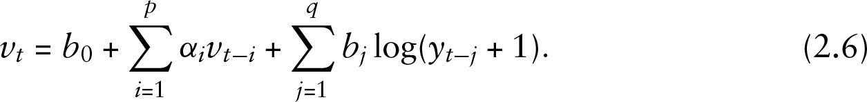
In this model, parameters
Ergodic properties of this model have been studied in Fokianos and Tjøstheim (2011). Stationarity conditions have been examined by Fokianos and Tjøstheim (2011), and they have been used by Liboschik et al.(2015)Liboschik, Fokianos, and Fried. Based on this work, we consider the stationarity conditions to be

Denote the available data up to time point
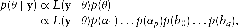
where
Given that
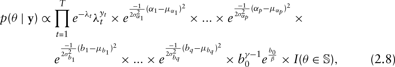
where
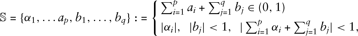
for the linear and the log-linear cases accordingly.
We use
where
While the literature on discrete valued time series is increasing very fast, there are very few papers that consider the problem of model selection, namely that of selecting the order of the model. In simple INAR(
In addition, Alzahrani et al.(2018)Alzahrani, Neal, Spencer, McKinley, and Touloupou studied the model selection problem among INAR and linear INGARCH models by using particle filtering MCMC method. Wang et al.(2020)Wang, Wang, and Zhang used a penalized conditional maximum likelihood to estimate the parameters of an INGARCH model. Note that this approach while can help to identify useful terms in the model, it does not select between competing models.
Prediction and Model averaging
Predictions in time varying volatility in linear and log-linear INGARCH models can be obtained from the output of the MCMC. McCabe and Martin (2005) studied methods for prediction of INAR(1) model. Raftery et al.(1997)Raftery, Madigan, and Hoeting discussed model averaging and the choice of models for Bayesian model averaging. A

where \ensuremath \cal M denotes the countable set of candidate models and

which is an average of the posterior predictive distribution under each model weighted by their posterior model probabilities. For each parameter vector, we calculate at each iteration
Assume that we have a countable set of models denoted by \ensuremath \cal M for a given set of data
Then posterior probability for model

where
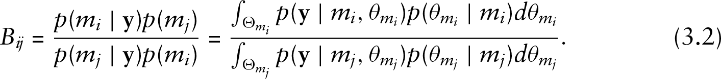
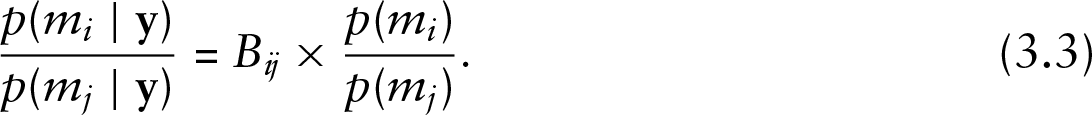
Second we could say that posterior model odds can be represented as
The integrals required for Bayes factor are analytically intractable. Consequently, many methods have been proposed to approximate Bayes factor. Methods introduced by Green (1995), Carlin and Chib (1995) and Dellaportas et al.(2002)Dellaportas, Forster, and Ntzoufras, generate observations from the joint posterior distribution from
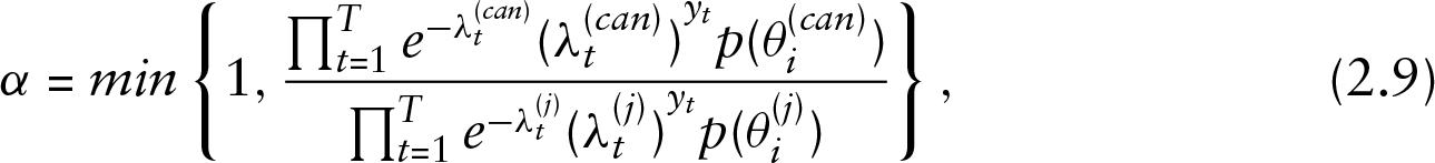
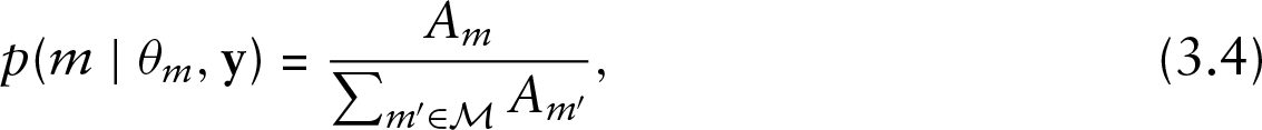
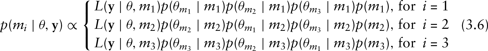
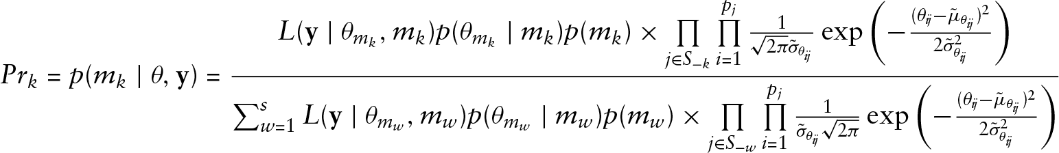
RJMCMC is a more complicated method in our case because we have a certain number of models, so an appropriate transformation is necessary to define each time the parameter spaces in order to make jumps between models. We do not pursue this in the present article. A method introduced by Carlin and Chib (1995) proposes jumps between all models. The full conditional posterior density for each model is given by
where numerator is given by equation

There are alternative constructions proposed by Bayarri et al.(2012)Bayarri, Berger, Forte, Garcí a-Donato, et al. in the case where the models are nested. Metropolized Carlin and Chib method proposes a move from one model to some other and examine the acceptance or rejection of this proposal. Lodewyckx et al.(2011)Lodewyckx, Kim, Lee, Tuerlinckx, Kuppens, and Wagenmakers suggested the product space method both in the cases of nested and non-nested models.
For example, let us consider three models, namely INGARCH(1,1), INGARCH(1,2) and INGARCH(2,1) denoted as
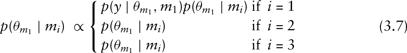
The crucial problem here is the matching of dimensions of the three models. For doing so we consider that if model

where
where
and
where
In this section, we present results from a small simulation experiment aiming at examining whether our approach can identify the correct structure of the time series that generated the data. We make use of sample size
Criterion 1: Each conditional prior must be proper (integrating to one) and cannot be arbitrarily vague in the sense of almost all of its mass being outside any believable compact set.
Criterion 2: (Model selection consistency) If data
If Criterion 2 is not accomplished a different choice of prior distributions is necessary. Recently, effort has been devoted to the choice of model priors. Bayarri et al.(2012)Bayarri, Berger, Forte, Garcí a-Donato, et al. and Consonni et al.(2018)Consonni, Fouskakis, Liseo, Ntzoufras, et al. proposed different choices of priors in objective Bayesian analysis. In our case, for the accomplishment of Criterion 1, we suggest as pseudopriors normal densities obtaining mean and variance after ‘pilot runs’ of MCMC for each model and considering that those pseudopriors are proper. More specifically, we generate 100 datasets of size
We present the results of averages based on 100 replications for each model. The columns correspond to the selected model out of 10 models, while the rows are the true models that generated the data. Note that in addition to the 10 INGARCH models we have two additional models different from INGARCH type. The first model was an INAR(2) model of the form
Looking at the results from Table 1, we can see that even for small sample size we can identify the correct structure with great success for most of the models. As expected in most cases when we do not identify the model that generated the data, the preferred model is one close (in the sense of the parameters set-up) which is reasonable.
Overall, the experiment shows that the method can identify the underlying model with good success.
Averages of posterior model probabilities after 100 samples of data from each model (multiplied by 100) where
is the class of linear and
of log-linear INGARCH models accordingly. Our approach correctly detects the model with high probability

Averages of posterior model probabilities after 100 samples of data from each model (multiplied by 100) where
is the class of linear and
of log-linear INGARCH models accordingly. Our approach correctly detects the model with high probability
Polio data
The data consist of monthly counts of poliomyelitis cases in the United States from 1970 to 1983 (168 observations) reported by the Centres for Disease Control and discussed in Zeger (1988) among others. Figure 1 presents the original series and the autocorrelation function of the series. In trans-dimensional method, we consider jumps between five linear and five log-linear INGARCH model.
Series of polio dataset (left) and its ACF (right)

Series of polio dataset (left) and its ACF (right)
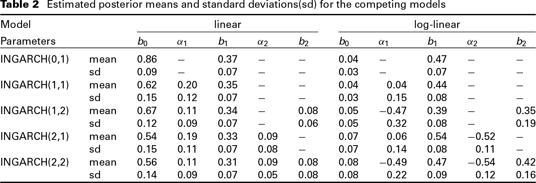
Table 2 presents estimators for each of five linear and log-linear INGARCH(
Estimated posterior means and standard deviations(sd) for the competing models
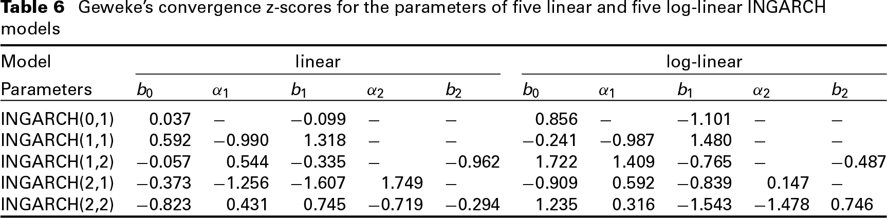
Geweke's convergence z-scores for the parameters of five linear and five log-linear INGARCH models

For the models where parameters satisfy stationarity conditions, we apply trans-dimensional MCMC method of Lodewyckx et al.(2011)Lodewyckx, Kim, Lee, Tuerlinckx, Kuppens, and Wagenmakers and posterior probabilities are presented in Table 4. The INGARCH(1,1) model is the one mostly visited which indicates that this is the selected model. Note that the 4 best models are of the linear type while the log-linear models have much smaller posterior probabilities.
Bayes factors are also reported in Table 4. They have been calculated with respect to the last (and more complicated) model. They also support simple models.
Posterior probabilities and Bayes factor for the competing models

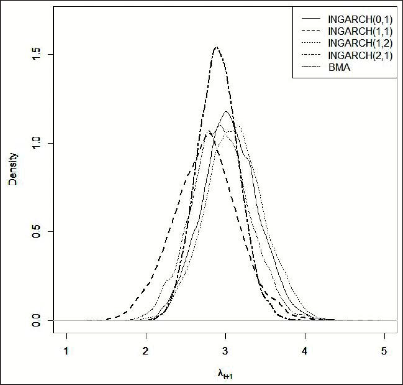
Finally, considering that we have posterior model probabilities for all models, we apply a Bayesian model-averaging (BMA) procedure. Based on posterior model probabilities, as estimated via trans-dimensional MCMC, we derive the density of predictive volatilities. Consequently, we calculate
Posterior density for
for polio data
The data (e.g., Liboschik et al.(2015)Liboschik, Fokianos, and Fried) consist of number of campylobacterosis cases in the North of Québec in Canada. Figure 3 presents the original series and the autocorrelation function of the series. Similarly, as for the polio dataset, we present parameters estimation and Z-scores concerning and checking the convergence. Considering the same conditions of stationarity as for the polio dataset, we present in Table 7 results after the trans-dimensional MCMC algorithm. In this case, we observe that the 4 best models are not only linear but also they have a complicated structure. Furthermore, the simple model INGARCH(1,0) is the less preferable. In Tables 5 and 6 one can see the posterior means and standard deviations as well as the Geweke's convergence diagnostics for the competing models.
Series of campylobacterosis dataset (left) and its ACF (right)

Series of campylobacterosis dataset (left) and its ACF (right)
Estimated posterior means and standard deviations(sd) for the competing models

Geweke's convergence z-scores for the parameters of five linear and five log-linear INGARCH models
Posterior probabilities and Bayes factor for the competing models

Posterior density for
for Campylobacterosis data

Finally, we have again calculated
We have developed a trans-dimensional MCMC approach for model selection between a family of Poisson INGARCH type models including linear and log-linear models. This allows to fit the models and select the one that best fits the data. Model selection for discrete valued time series is a topic of less research, and we think that we contribute towards this. Our approach is based on satisfying the stationarity conditions, that is, assuming that the series are stationary. Allowing for combinations of parameters beyond stationarity is possible but the interpretation of the models is more difficult afterwards.
The method that has been discussed by Carlin and Chib (1995) is the most flexible method in our case when we have a number of nested models. This is an important issue because since now there are limited studies about trans-dimensional methods for count data.
Furthermore we note that, although we only analysed methodology by using linear and log-linear INGARCH models when all parameters are positive, our analysis can be extended when parameters are negative in case of log-linear INGARCH models. In addition, the use of other functions for the mean process
Finally, in the present article, we treated only Poisson INGARCH models. However, the method can be easily extended to the case of other models of the same type with different conditional distributions that have appeared in the literature.
Appendix A: MCMC for the general INGARCH model
Denote as
We use Initialize For the ( Generate values from proposal densities for Update Iterate this updating procedure. Go to the next iteration or stop if the chain has converged.
Appendix B: The transdimensional MCMC
Consider
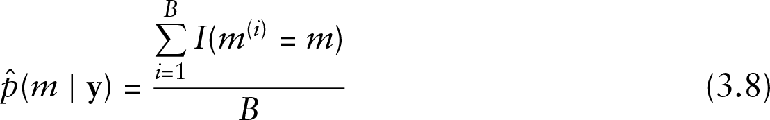
For a number of iterations say For model We repeat this for each candidate model so for all Calculate posterior probability for model We select the model with larger value Repeat steps 1–4 for At the end calculate s posterior model probabilities given by (3.8)
Footnotes
Declaration of conflicting interests
The authors declared no potential conflicts of interest with respect to the research, authorship and/or publication of this article.
Funding
The author(s) received no financial support for the research, authorship, and/or publication of this article.
Acknowledgments
This research is co-financed by Greece and the European Union (European Social Fund [ESF]) through the Operational Programme ≪Human Resources Development, Education and Lifelong Learning≫ in the context of the project ‘Strengthening Human Resources Research Potential via Doctorate Research’ (MIS-5000432), implemented by the State Scholarships Foundation (IKY). The second author Dimitris Karlis received a grant from the Research Center of the Athens University of Economics and Business under the project ‘Innovative Publications’.