A joint transition model for evaluating eGFR as biomarker for rejection after kidney transplantation

Abstract

The estimated glomerular filtration rate (eGFR) quantifies kidney graft function and is measured repeatedly after transplantation. Kidney graft rejection is diagnosed by performing biopsies on a regular basis (protocol biopsies at time of stable eGFR) or by performing biopsies due to clinical cause (indication biopsies at time of declining eGFR). The diagnostic value of the eGFR evolution as biomarker for rejection is not well established. To this end, we built a joint model which combines characteristics of transition models and shared parameter models to carry over information from one biopsy to the next, taking into account the longitudinal information of eGFR collected in between. From our model, applied to data of University Hospitals Leuven (870 transplantations, 2 635 biopsies), we conclude that a negative deviation from the mean eGFR slope increases the probability of rejection in indication biopsies, but that, on top of the biopsy history, there is little benefit in using the eGFR profile for diagnosing rejection. Methodologically, our model fills a gap in the biomarker literature by relating a frequently (repeatedly) measured continuous outcome with a less frequently (repeatedly) measured binary indicator. The developed joint transition model is flexible and applicable to multiple other research settings.

Keywords

biomarker research Kidney rejection joint modelling transition model shared parameters

1 Introduction

Observational data, usually comprising of the longitudinal follow-up of a cohort, is one of the main data sources in kidney transplantation research. Apart from baseline information at the day of transplantation, parameters on renal function, like estimated glomerular filtration rate (eGFR) and proteinuria, are collected repeatedly at the occasion of clinical visits in order to detect and treat allograft injury. Via biopsies, performed in case of a clinical indication of renal graft injury (declining eGFR or increasing proteinuria), the so-called indication biopsies, data on kidney histology and rejection phenotypes are obtained as well. Next to indication biopsies, many centres also collect biopsies per protocol, leading to a less selected view on the progression of kidney histology post transplantation (Racusen, 2006; Wilkinson, 2006). Due to the invasiveness of biopsies, histological data are more scarce than data on renal functioning.

In recent years, there is an increased interest in the discovery of non-invasive biomarkers for acute and chronic rejection and chronic allograft injury after kidney transplantation (Salvadori and Tsalouchos, 2017; Van Loon et al., 2019). Advances in ‘omics’ research, for example, led to robust, predictive and useful biomarkers at the molecular level (Salvadori and Tsalouchos, 2017). A clinically useful non-invasive biomarker should allow for the early discovery of future kidney damage/failure and should be sufficiently sensitive. A well-performing biomarker for kidney histology could eliminate the need for conducting invasive biopsies (Lo et al., 2014; Peters et al., 2014; Lopez-Giacoman and Madero, 2015).

When conceiving renal functional parameters as a continuous biomarker for the presence or absence of kidney rejection at the time of biopsy, these data can be viewed as recurrent longitudinal sequences of marker measurements with binary indicators (rejection or not) in between. After all, rejection is not a final end-point. Jointly analyzing these outcomes requires the specification of their multivariate distribution. However, this specification is hampered because both responses are irregularly measured variables of a different type (continuous and binary). A popular approach for jointly modelling two longitudinal processes of a different type, and widely applied in biomarker discovery (Li et al., 2017), is the shared parameter model, which assumes conditional independence given a common set of random effects. These models are advantageous in the sense that the parameter estimates of the separate models can be interpreted as if they were modelled separately. A typical example is the joint longitudinal survival model, where a longitudinal continuous marker is correlated with a time-to-event outcome (Rizopoulos, 2011, 2012; Li et al., 2017). Extensions of the joint longitudinal survival model were made to include recurrent events (Liu and Huang, 2009; Kim et al., 2012), competing risks (Elasho et al., 2008; Rizopoulos, 2012) and multi-state models (Ferrer et al., 2016). In some cases, this time-to-event outcome can even be downgraded to a binary outcome. Examples can be found in Horrocks and van Den Heuvel, 2009 where a successful pregnancy was predicted from the adhesiveness of certain blood lymphocytes, or in Chen et al., 2015 where the development of self-esteem was related to anxiety disorder at a certain age. Yet, when the binary outcome is also measured longitudinally, a random-effects approach (Verbeke et al., 2014) is often preferred. By including separate, but correlated random effects, these models allow for more flexibility in the correlation structure between both longitudinal processes. An example can be found in Gueorguieva, 2001 where malformation (binary) and birth weight (continuous) of mice foetuses were associated with a certain toxic dose.

Instead of using a mixed model for the binary outcome, as in the random-effects approach, another valuable model for occasionally measured, longitudinal outcomes, is the transition model (Verbeke et al., 2014). Univariate transition models factorize the joint distribution of a longitudinal outcome into the marginal distribution for the first response and a set of conditional distributions for the later responses given the earlier ones (Diggle et al., 2002; Molenberghs and Verbeke, 2006; de Rooij, 2018). In case of categorical outcomes, transition models consider the data as a sequence of states (Liang and Zeger, 1989), which exactly corresponds to the research setting of recurrent biopsy data. In joint modelling, the use of transition models instead of mixed models is advantageous especially during the fitting process. Random-effects models require the specification of multiple, often complex, random effects structures, leading to intractable integrals in the likelihood. Transition models on the contrary allow for dependence in a sequence of states via a fixed parameter structure. In addition, transition models allow for a predictive interpretation, that is, using past measurements to determine future events, a property which is much more difficult to attain in a random-effects approach.

Combining characteristics of the transition model with these of the shared parameter model for evaluating a potential biomarker for a histological outcome is, to the best of our knowledge, never implemented before and will be addressed in this article. By doing so, we provide a new methodological framework for modelling the multivariate distribution of a frequently (repeatedly) measured continuous response and a less frequently (repeatedly) measured binary response, applied to a use case in kidney transplantation.

2 Motivating case study

At the University Hospitals Leuven, for kidney transplant recipients, an intensive protocol biopsy program has been established since 2004. On top of indication biopsies, performed in case of clinical suspicion, the staff decided on pre-planned biopsies at day 0, 3 months, 1 year and then every year up to 5 years post transplantation. By doing so, a full longitudinal picture of a patient's kidney histology is obtained, which is then used to diagnose transplant rejection. For this study, all single kidney transplantations performed between March 2004 and February 2013 were eligible. Recipients were included if they had at least two performed biopsies after baseline, at least one kidney function measurement in between every biopsy and complete data on the status of pre-transplant donor-specific antibodies (DSA). For each included biopsy, full data on the rejection type was required. In total, we disposed of 2 635 biopsies, 463 of which were indication biopsies, in 870 patients, and of 40.649 eGFR measurements. The inclusion flow chart is displayed in Figure 1.

Figure 1:

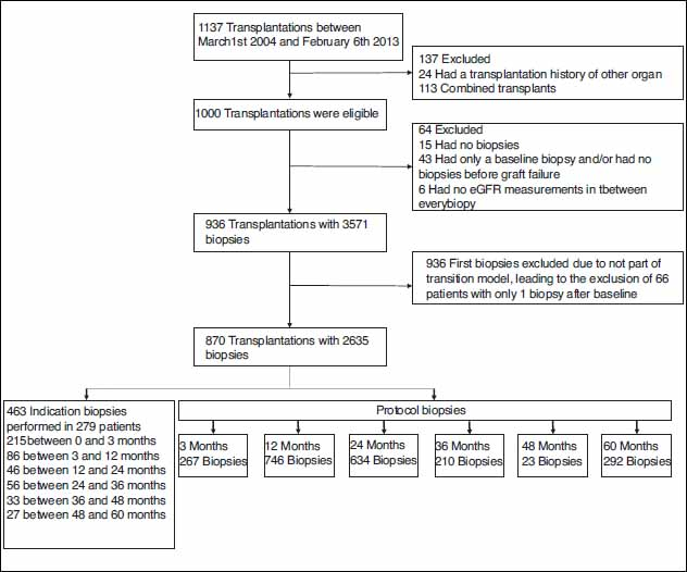
Inclusion flow chart. Indication biopsies were performed in case of clinical suspicion while protocol biopsies were pre-planned

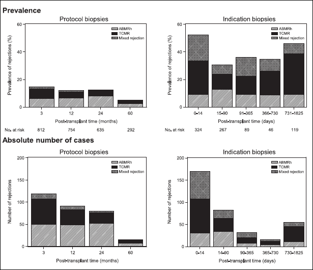
In renal transplantation, two main types of rejection are distinguished: antibody-mediated rejection (ABMR) and T-cell mediated rejection (TCMR) (Loupy et al., 2020). For the latter, effective treatment is available, while the first lacks efficacious therapy (Djamali et al., 2014; Van Loon et al., 2020). Both types of rejection can occur at any time after transplantation. Figure 2 shows the prevalence of ABMRh (=histological picture of ABMR as defined by the Banff 2019 classification without considering the DSA status), TCMR and mixed rejection in the Leuven cohort, indicating that any type of rejection occurs more frequently in indication than in protocol biopsies. In addition, it is clear that in the unselected (protocol) cohort the prevalence of rejection decreases by time. In indication biopsies, there is no time trend in the prevalence, showing their informative measurement. It has been shown that previous episodes of acute rejection are a risk factor for rejections in the future (Joosten et al., 2005).

Figure 2:

Prevalence of rejection in protocol and indication biopsies in the Leuven cohort (3 571 biopsies in 936 patients). Indication biopsies were performed in case of clinical suspicion while protocol biopsies were pre-planned. ABMRh = Histological picture of ABMR as defined by the Banff 2019 criteria, TCMR = T-cell mediated rejection, Mixed rejection = ABMRh and TCMR

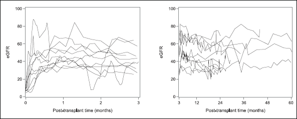
The clinical decision for proceeding to an indication biopsy is mostly based on poor or worsening kidney function, measured by eGFR. Figure 3 shows 10 randomly sampled eGFR profiles from the Leuven cohort, separately for the first three months after transplantation, and afterwards. There is an upward trend of kidney function shortly after transplantation, followed by a stabilizing period. After three months, eGFR exerts little variation in time. By definition, protocol biopsies are performed in patients with stable eGFR. As rejection occurs more often in indication biopsies than in protocol biopsies (Halloran et al., 2019), eGFR is expected to have at least some predictive value for the diagnosis of rejection, although eGFR was shown to be a rather insensitive biomarker of renal injury (Fassett et al., 2011; Loupy et al., 2015; Hollis et al., 2017). The lack of sensitivity of eGFR for kidney injury and rejection could be related to the fact that most studies in transplantation relate eGFR only at one fixed point in time to graft failure or histological outcomes (Viglietti et al., 2018; Loupy et al., 2019; Einecke et al., 2020), hence not considering its longitudinal profile. Other studies correlate renal function at 1-year post transplantation with late graft failure (Hariharan et al., 2002; Kasiske et al., 2002; Loupy et al., 2015). Even more, we found no statistical models that relate a longitudinal biomarker with a recurrent biopsy outcome.

Figure 3:

10 randomly sampled recipients’ eGFR profiles from the Leuven cohort (n=936). eGFR, as a measure for renal function, is measured in ml/min/1.73mÃÂ² according to the MDRD formula. The left panel shows the eGFR evolution in the first three months after transplantation. The right panel shows the eGFR evolution afterwards

The fact that no statistical algorithms for kidney allograft rejection were developed or implemented in clinical practice reflects the difficulty of its early diagnosis. The discovery of baseline risk factors, like the presence of DSA or the number of HLA mismatches, has not led to a sufficiently sensitive/specific marker for acute or chronic rejection. The inclusion of time-dependent information is therefore an essential next step. On top of the (time-dependent) biopsy history, longitudinal biomarkers have the potential of increasing the predictive power of a model by including information that is not always obvious during visual inspection. The increase or decrease of a longitudinal profile may be alarming for one person, but not necessarily for another. Hence, there is a need for a model that objectifies the risk estimate of rejection, based on longitudinal information contained in a potential biomarker, on top of the biopsy history. Once established, the model should be able to detect important biomarkers and should be extendable to multiple biomarkers. In our case, we aim at predicting kidney transplant rejection (ABMRh and/or TCMR) based on the prior rejection history and on the eGFR evolution. The rejection history is a well-known, time-dependent risk factor, while eGFR is a potential longitudinal biomarker. Statistically, the challenge comprises of combining the two longitudinal processes in one model, while adhering to a causal framework that only conditions on the past.

In the following sections, we present a modelling framework that combines transitional components with shared parameters in order to flexibly model the information carried from one biopsy to the next, taking into account the longitudinal information about renal functioning, collected in between the biopsies. Concerning inference, we expect our model to evaluate the importance of (longitudinal) eGFR in determining allograft rejection in a subsequent biopsy. Regarding prediction, we expect our proposed model to outperform a model in which the longitudinal information of eGFR is not included.

3 Methodology

3.1 Likelihood factorization and random effects

We propose the use of a joint model in which we combine characteristics of transition models, together with characteristics of shared parameter models in order to specify the multivariate distribution of the rejection outcomes and eGFR profiles. First, we define the likelihood function, in which we incorporate all available information. We denote the vector of eGFR measurements in period $j$ as $Y_{j}$ and the biopsy outcome (rejection or not) at the end of that period as $B_{j}$ . In order to keep notation simple, we suppress an index i for subject in the dataset. Hence, for each period j, the measurements are defined as ( $Y_{j}$ , $B_{j}$ ). The likelihood contribution of a patient with p sequences of longitudinal eGFR measures followed by a biopsy is therefore equal to:

\begin{matrix} L & = & f [(Y_{1}, B_{1}), (Y_{2}, B_{2}), \dots, (Y_{j}, B_{j}), \dots, (Y_{p}, B_{p})], \end{matrix}

(3.1)

which can easily be factorized as

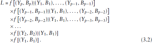
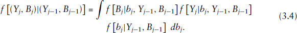
\begin{matrix} L & = & f [(Y_{p}, B_{p}) | (Y_{1}, B_{1}), \dots, (Y_{p - 1}, B_{p - 1})] \\ \times f [(Y_{p - 1}, B_{p - 1}) | (Y_{1}, B_{1}), \dots, (Y_{p - 2}, B_{p - 2})] \\ \times f [(Y_{p - 2}, B_{p - 2}) | (Y_{1}, B_{1}), \dots, (Y_{p - 3}, B_{p - 3})] \\ \times \dots \\ \times f [(Y_{2}, B_{2}) | (Y_{1}, B_{1})] \\ \times f [(Y_{1}, B_{1})] . \end{matrix}

(3.2)

This type of factorization avoids the need for the direct specification of the joint likelihood (Diggle et al., 2002; Serroyen et al., 2009; Verbeke et al., 2014) by conditioning the outcome on other outcomes or on a subset of these (Fitzmaurice and Molenberghs, 2009). In case of longitudinal data, the factorization leads to the so-called transition model in which the current outcome is conditioned on the past responses. Indeed, rejection and the eGFR values in period j depend on the previous biopsies and eGFR measurements. This approach is natural to our research question in which we want to use historic information in order to predict future rejection. A common assumption in the transition model is the first-order autoregressive structure, AR(1), which indicates that the distribution of the measurements in period j only depends on the measurements taken in the preceding period and not on those taken in earlier periods. Clinically, this assumption is plausible since therapeutic decisions are usually made on the last biopsy outcome and the recent foregoing eGFR trajectory. Nevertheless, because the eGFR profile and biopsy outcome of period j-1 depend on the outcomes of period j-2, implicitly non-neighbouring periods are still associated. More specifically, we assume that

\begin{matrix} f [(Y_{j}, B_{j}) | (Y_{1}, B_{1}), \dots, (Y_{j - 1}, B_{j - 1})] & = & f [(Y_{j}, B_{j}) | (Y_{j - 1}, B_{j - 1})] . \end{matrix}

(3.3)

In addition to the previously proposed transition structure, we assume that the association between the longitudinal eGFR process ( $Y_{j}$ ) and the biopsy outcome ( $B_{j}$ ) in period j can be captured with latent random effects ( $b_{j}$ ), thereby assuming conditional independence. These random effects reflect the patient-specific deviations from the mean eGFR trajectory in period j and can likely explain the dependence between eGFR and rejection. As such, the conditional joint distribution of eGFR and the biopsy outcome is modelled using a shared parameters model. More specifically, we assume that (3.3) factorizes as

\begin{matrix} f [(Y_{j}, B_{j}) | (Y_{j - 1}, B_{j - 1})] & = \int f [B_{j} | b_{j}, Y_{j - 1}, B_{j - 1}] f [Y_{j} | b_{j}, Y_{j - 1}, B_{j - 1}] \\ f [b_{j} | Y_{j - 1}, B_{j - 1}] d b_{j} . \end{matrix}

(3.4)

3.2 Extra modelling assumptions

Finalizing the likelihood expression in (3.4) requires the explicit modelling of every factor in the equation. The last factor pertains to the random effects resulting from a mixed model for eGFR, which are assumed not to be affected by the eGFR measurements or biopsy outcome in the previous period, that is,

\begin{matrix} f [b_{j} | Y_{j - 1}, B_{j - 1}] & = & f [b_{j}], \end{matrix}

(3.5)

where $b_{j}$ is assumed to be normally distributed with mean 0 and covariance matrix D.

When the decision for a biopsy is based on an eGFR deviation (indication biopsy), it is plausible to assume that only the measurements of the current period are predictive for rejection. Likewise, in case of a protocol biopsy with stable eGFR, also the current measurements will suffice for predicting the biopsy outcome. Hence, in modelling terms, we assume the rejection status in period j to depend on the previous biopsy and on the random effects of that same period:

\begin{matrix} f [B_{j} | b_{j}, Y_{j - 1}, B_{j - 1}] & = & f [B_{j} | b_{j}, B_{j - 1}] . \end{matrix}

(3.6)

Finally, we assume that a summary $a (Y_{j - 1})$ of the longitudinal eGFR measurements in the previous period is sufficient to predict eGFR in the current period, conditionally on the random effects $b_{j}$ and the past biopsy outcome, that is,

\begin{matrix} f [Y_{j} | b_{j}, Y_{j - 1}, B_{j - 1}] & = & f [Y_{j} | b_{j}, B_{j - 1}, a (Y_{j - 1})] . \end{matrix}

(3.7)

This solves the issue of having to condition on a vector

Y_{j - 1}

which is not of a fixed dimension. Note that the summary a(.) can be multi-dimensional and will be selected such that it captures the most important information in the eGFR trend during one period to predict the trend in the next period.

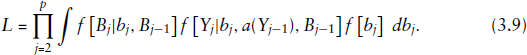
Combining expressions (3.3) to (3.7) and substituting these in (3.2) results in a likelihood contribution of each individual patient of:

\begin{matrix} \begin{matrix} L & = & f [(Y_{1}, B_{1})] \times \prod_{j = 2}^{p} \int f [B_{j} | b_{j}, B_{j - 1}] f [Y_{j} | b_{j}, a (Y_{j - 1}), B_{j - 1}] f [b_{j}] d b_{j} . \end{matrix} \end{matrix}

(3.8)

Because eGFR shows a very different trajectory in the first days after transplantation compared to afterwards, the first factor would need to be modelled completely separately from the second factor, and therefore can be ignored when interests are in predictions after the stabilizing period. Therefore, the final likelihood simplifies to:

\begin{matrix} L & = & \prod_{j = 2}^{p} \int f [B_{j} | b_{j}, B_{j - 1}] f [Y_{j} | b_{j}, a (Y_{j - 1}), B_{j - 1}] f [b_{j}] d b_{j} . \end{matrix}

(3.9)

4 Fitting the joint transition model

4.1 eGFR modelling choices

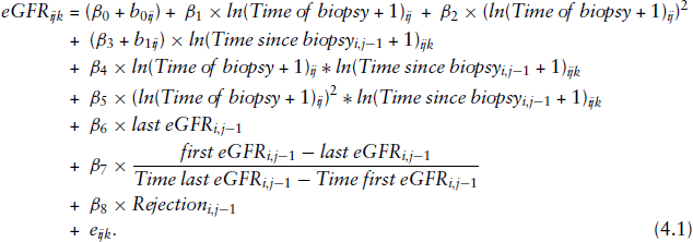
As eGFR is a continuous measure and rejection is binary (present/absent), we propose to jointly model a Gaussian linear mixed model with a logistic regression (transition) model. In the linear mixed model we include two time effects (in years): one models the timing of the biopsy at the end of the period under consideration and one models the timing of the eGFR measurement since the previous biopsy. Since the eGFR trajectory first increases in the initial post-transplant phase, and consequently decreases slowly, both ‘Time of biopsy’ and ‘Time since biopsy’ were log-transformed. In order to achieve extra flexibility in the time trend we also included the quadratic form of ‘ln(Time of biopsy+1)’ and the interaction with ‘ln(Time since biopsy+1)’. The vector $a (Y_{j - 1})$ is expressed by using the last eGFR measurement of period j-1 and the difference between the first and the last eGFR measurement of period j-1 scaled by the length of period j-1. Finally, we also let the biopsy outcome in period j-1 to be related to the eGFR profile in period j. Concerning random effects, we assume normally distributed random intercepts and linear random slopes for ‘ln(Time since biopsy+1)’ both at the level of period, nested within subject. Note that the association between periods within subjects is assumed to be captured by the transitional component and hence no random effects at the subject level are included. The random effects $b 0_{ij}$ and $b 1_{ij}$ therefore reflect how the intercept and slope deviate from the intercept and slope of the average eGFR profile in period j, for patient i. The linear model for the $k$ th eGFR value during period j for patient i is then given by

\begin{matrix} {eGFR}_{ijk} & = & (β_{0} + b_{0 ij}) + β_{1} \times \ln (Time of biopsy + 1)_{ij} + β_{2} \times (\ln (Time of biopsy + 1)_{ij})^{2} \\ + & (β_{3} + b_{1 ij}) \times \ln (Time since {biopsy}_{i, j - 1} + 1)_{ijk} \\ + & β_{4} \times \ln (Time of biopsy + 1)_{ij} * \ln (Time since {biopsy}_{i, j - 1} + 1)_{ijk} \\ + & β_{5} \times (\ln (Time of biopsy + 1)_{ij})^{2} * \ln (Time since {biopsy}_{i, j - 1} + 1)_{ijk} \\ + & β_{6} \times {last eGFR}_{i, j - 1} \\ + & β_{7} \times \frac{first {eGFR}_{i, j - 1} - last {eGFR}_{i, j - 1}}{Time last {eGFR}_{i, j - 1} - Time first {eGFR}_{i, j - 1}} \\ + & β_{8} \times {Rejection}_{i, j - 1} \\ + & e_{ijk} . \end{matrix}

(4.1)

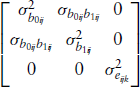
We further assume that the vector ( $b_{0 ij}$ , $b_{1 ij}$ , $e_{ijk}$ ) is normally distributed with mean zero and covariance

[\begin{matrix} σ_{b_{0 ij}}^{2} & σ_{b_{0 ij} b_{1 ij}} & 0 \\ σ_{b_{0 ij} b_{1 ij}} & σ_{b_{1 ij}}^{2} & 0 \\ 0 & 0 & σ_{e_{ijk}}^{2} \end{matrix}]

4.2 Rejection modelling choices

For rejection, a logistic regression model is used. As the prevalence of rejection is decreasing by time after transplantation, we assume a linear effect of the timing of biopsy on the logit for rejection. Also, the previous biopsy outcome and the presence of pre-transplant DSA are included in the model. The random intercepts ( $b_{0 ij}$ ) and slopes ( $b_{1 ij}$ ) of the eGFR profiles are introduced into the model, directly interacting with the variable ‘Protocol vs Indication biopsy’, allowing their effects to be different for indication and protocol biopsies. Since the type of biopsy partly depends on the eGFR profile, this separation seems justified. The part of our model relating to rejection of patient i in period j therefore is given by

\begin{matrix} Logit (Any Rejection)_{ij} & = & γ_{0} + γ_{1} \times Time of {biopsy}_{ij} \\ + & γ_{2} \times b_{0 ij} \times (1 - (Protocol [0] vs . Indication [1] biopsy)_{ij}) \\ + & γ_{3} \times b_{1 ij} \times (1 - (Protocol [0] vs . Indication [1] biopsy)_{ij}) \\ + & γ_{4} \times b_{0 ij} \times (Protocol [0] vs . Indication [1] biopsy)_{ij} \\ + & γ_{5} \times b_{1 ij} \times (Protocol [0] vs . Indication [1] biopsy)_{ij} \\ + & γ_{6} \times {Rejection}_{i, j - 1} \\ + & γ_{7} \times Pre - transplant {DSA}_{i} . \end{matrix}

(4.2)

4.3 Results

The procedure NLMIXED in SAS (v9.4; SAS Institute) is used to perform the analyses. In Supplemental Material (http://www.statmod.org/smij/archive.html), this code is made available. Data can only be shared via a Data Transfer Agreement, after having contacted the authors. Joint significance testing was done via approximate F tests using the delta method (Cox, 1998) to approximate the variance-covariance matrix. Inference on the covariance and correlation of the random effects was done via t-tests, in which the standard errors of the estimates were approximated using the delta method (Billingsley, 1986). 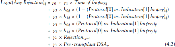Table 1 shows the estimates of the joint transition model. All fixed effects in the eGFR sub-model (the $β$ ’s) are significant. Note however that interpretation of individual parameters is hampered by the fact that the model includes higher-order terms and interactions. Therefore, in order to evaluate the performance of the model, we show in Figure 4 the eGFR profiles of three randomly selected subjects, together with their estimated lines according to the model. It is clear that the observed eGFR profiles were well approximated by the model. The curves are not smooth, which is to be expected since we use a transition model that divides the time course in intervals defined by the biopsies, and we do no impose any smoothing restrictions.

Figure 4:

Modelled (joint transition model) and observed eGFR profiles of three randomly selected recipients. eGFR, as a measure for renal function, is measured in ml/min/1.73mÃÂ² according to the MDRD formula

In the sub-model for rejection (the $γ$ ’s), we observe that there is a significant downward trend in time, together with an increased probability of rejection when the previous biopsy was positive, and the patient had pre-transplant DSA. Yet, of most interest to us are the scaling parameters with relation to the random effects ( $γ_{2}$ - $γ_{5}$ ). $γ_{2}$ and $γ_{3}$ show that there is no significant effect of either the random intercepts or the random slopes of the eGFR profiles for the prediction of rejection in protocol biopsies (joint p-value: $p = 0.444$ ). As eGFR in protocol biopsies is stable by definition, the non-significance of the slopes was to be expected. However, our model now also confirms there is no effect of the level of eGFR. On the contrary, for indication biopsies ( $γ_{4}$ - $γ_{5}$ ) we show that there is an effect of the random effects parameters on the probability of rejection (joint p-value: $p = 0.004$ ). More specifically, deviating positively from the mean slope of eGFR ( $γ_{5}$ ) decreases the chances for rejection ( $p = 0.001$ ). This makes sense in an upward, as well as in a downward trend: if eGFR is increasing, a negative slope deviation (slower incline) evidently should lead to a higher probability of rejection. If eGFR is decreasing, a negative slope deviation (faster decline) should also lead to a higher probability of rejection.

Next, it is of interest how well our model performs in terms of prediction. Rejection probabilities in the joint transition model are calculated based on the entire history, which is captured by the eGFR random effects and the previous biopsy outcome, that is, $P$ ( $B_{j}$ = 1 $|$ $b_{j}$ , $B_{j - 1}$ ). In Figure 5, we compare the ROC curve of our joint transition model (AUC=0.75) with the one of the univariate, AR(1), transition model ( $P$ ( $B_{j}$ = 1 $| B_{j - 1}$ )), that is, not including eGFR in the model (AUC=0.74). As was expected from the non-significant estimates in Table 1, the added value of the eGFR trajectories is minimal, hence showing little improvement for classification. Nonetheless, since the eGFR profiles only contribute to predicting rejection in indication biopsies, in Figure 6 we plotted the same ROC curves for protocol and indication biopsies separately. For protocol biopsies, the AUC is 0.71 for the joint transition model, while being 0.72 for the univariate transition model. For indication biopsies, the AUC's were 0.72 and 0.68 respectively. Hence, for the latter, although minimal, there is some added value for classification. Yet, a fair evaluation of our model should point to the fact that the overall predictive ability is mediocre, and that little extra information is contained in the longitudinal profile of eGFR, on top of the univariate transition model, for determining rejection.

Figure 5:

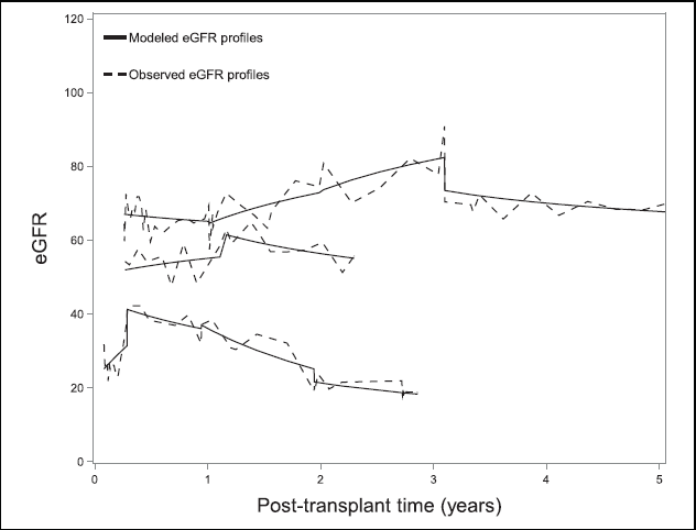
General ROC curve comparison between the joint transition model and the marginal model (= univariate transition model) for predicting kidney allograft rejection (ABMRh and/or TCMR). The marginal model (AUC = 0.74) contains the timing of the biopsy, rejection in the previous biopsy (yes/no) and the presence or absence of pre-transplant DSA (based on 2 635 biopsies, in 870 patients). The joint transition model (AUC = 0.75) contains the same parameters + the eGFR trajectories (based on 2 635 biopsies and 40.649 eGFR values, in 870 patients)

Figure 6:

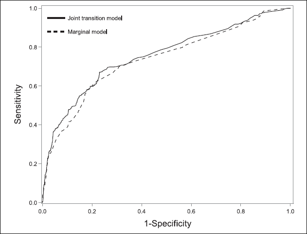
ROC curve comparison between the joint transition model and the marginal model (= univariate transition model), separately for protocol and indication biopsies for predicting kidney allograft rejection (ABMRh and/or TCMR) The marginal model (AUC = 0.72 for protocol biopsies and 0.68 for indication biopsies) contains the timing of the biopsy, rejection in the previous biopsy (yes/no) and the presence or absence of pre-transplant DSA (based on 2 635 biopsies, in 870 patients). The joint transition model (AUC = 0.71 for protocol biopsies and 0.72 for indication biopsies) contains the same parameters + the eGFR trajectories (based on 2 635 biopsies and 40.649 eGFR values, in 870 patients)

Based on the non-significance of the correlation between random intercepts and slopes, we also fitted a model assuming independence, leading to similar inferences and predictive power (AUC = 0.76 in general, AUC = 0.71 in protocol biopsies and AUC = 0.73 in indication biopsies).

Table 1:

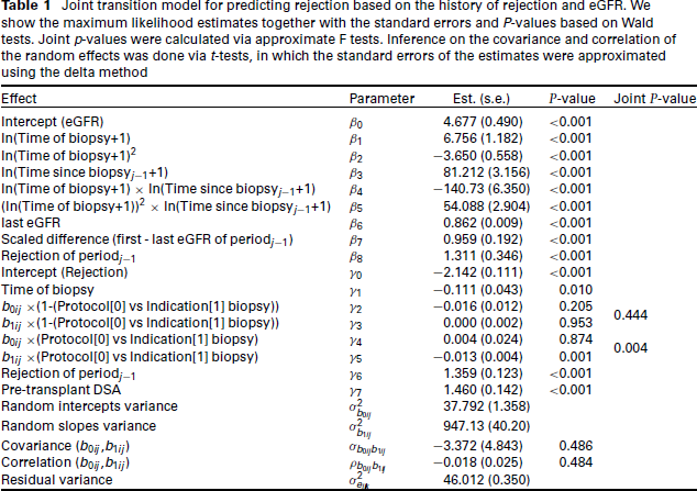
Joint transition model for predicting rejection based on the history of rejection and eGFR. We show the maximum likelihood estimates together with the standard errors and P-values based on Wald tests. Joint p-values were calculated via approximate F tests. Inference on the covariance and correlation of the random effects was done via t-tests, in which the standard errors of the estimates were approximated using the delta method

Effect	Parameter	Est. (s.e.)	P-value	Joint P-value
Intercept (eGFR)	$β_{0}$	4.677 (0.490)	$<$ 0.001
ln(Time of biopsy+1)	$β_{1}$	6.756 (1.182)	$<$ 0.001
ln(Time of biopsy+1) $^{2}$	$β_{2}$	$-$ 3.650 (0.558)	$<$ 0.001
ln(Time since biopsy $_{j - 1}$ +1)	$β_{3}$	81.212 (3.156)	$<$ 0.001
ln(Time of biopsy+1) $\times$ ln(Time since biopsy $_{j - 1}$ +1)	$β_{4}$	$-$ 140.73 (6.350)	$<$ 0.001
(ln(Time of biopsy+1)) $^{2}$ $\times$ ln(Time since biopsy $_{j - 1}$ +1)	$β_{5}$	54.088 (2.904)	$<$ 0.001
last eGFR	$β_{6}$	0.862 (0.009)	$<$ 0.001
Scaled difference (first - last eGFR of period $_{j - 1}$ )	$β_{7}$	0.959 (0.192)	$<$ 0.001
Rejection of period $_{j - 1}$	$β_{8}$	1.311 (0.346)	$<$ 0.001
Intercept (Rejection)	$γ_{0}$	$-$ 2.142 (0.111)	$<$ 0.001
Time of biopsy	$γ_{1}$	$-$ 0.111 (0.043)	0.010
$b_{0 ij}$ $\times$ (1-(Protocol[0] vs Indication[1] biopsy))	$γ_{2}$	$-$ 0.016 (0.012)	0.205	0.444
$b_{1 ij}$ $\times$ (1-(Protocol[0] vs Indication[1] biopsy))	$γ_{3}$	0.000 (0.002)	0.953
$b_{0 ij}$ $\times$ (Protocol[0] vs Indication[1] biopsy)	$γ_{4}$	0.004 (0.024)	0.874	0.004
$b_{1 ij}$ $\times$ (Protocol[0] vs Indication[1] biopsy)	$γ_{5}$	$-$ 0.013 (0.004)	0.001
Rejection of period $_{j - 1}$	$γ_{6}$	1.359 (0.123)	$<$ 0.001
Pre $-$ transplant DSA	$γ_{7}$	1.460 (0.142)	$<$ 0.001
Random intercepts variance	$σ_{b_{0 ij}}^{2}$	37.792 (1.358)
Random slopes variance	$σ_{b_{1 ij}}^{2}$	947.13 (40.20)
Covariance ( $b_{0 ij}$ , $b_{1 ij}$ )	$σ_{b_{0 ij} b_{1 ij}}$	$-$ 3.372 (4.843)	0.486
Correlation ( $b_{0 ij}$ , $b_{1 ij}$ )	$ρ_{b_{0 ij} b_{1 ij}}$	$-$ 0.018 (0.025)	0.484
Residual variance	$σ_{e_{ijk}}^{2}$	46.012 (0.350)

5 Conclusion and discussion

In this article, we developed a transition model with shared parameters in order to evaluate the predictive ability of biopsy history and eGFR for kidney transplant rejection. We confirmed the results reported before, showing that rejection in the previous biopsy and the presence of pre-transplant DSA increase the probability of rejection in the next biopsy. In addition, we confirmed the known fact that the chance of rejection decreases with time post transplantation. Concerning kidney function, evaluated using eGFR trajectories, we found that negatively deviating from the mean slope increases the probability of rejection in indication biopsies. Notwithstanding the significance of the latter effect, the added predictive ability of eGFR was minimal in comparison to a univariate transition model, excluding eGFR. Overall, the classification ability of the joint transition model is mediocre.

By fitting the joint transition model, we responded to the clinical question whether eGFR profiles are predictive for kidney allograft rejection. We showed that, next to the biopsy history, the additional information of longitudinally measured eGFR is rather insensitive for rejection. This opposes our hypothesis that the information contained in the eGFR trajectories would benefit the prediction of rejection, outperforming traditional statistical techniques, which not consider the time-evolution of eGFR. Nevertheless, traditional statistical techniques are not capable of making these complex inferences on the relation between the two longitudinal processes. More specifically, our model allowed to evaluate the strength of the relation between a recurrent biopsy outcome and a longitudinal biomarker and it was able to evaluate the predictive ability of this biomarker. In fact, we are the first to build a joint transition model for studying the association between a longitudinally measured (continuous) biomarker and a recurrent (binary) biopsy outcome. Concretely, we combined a transition model, accounting for historical information in the previous biopsies and eGFR trajectories, with a shared parameter model that correlated characteristics of the current eGFR profile with subsequent rejection.

In kidney transplantation, there is a need for accurate non-invasive biomarkers for rejection and graft failure. Research often focuses on blood or urine biomarkers for rejection at the time of biopsy, or on time-fixed predictors, usually measured at the day of transplantation. Few studies take advantage of the multiple biopsies per patient, or, when they do so, ignore the dependence between the measurements. On top, few studies make use of the multiple measurements of a biomarker. We suggest to focus on the longitudinal information contained in current and new biomarkers and on the combination of these into one model. Trajectory changes in biomarkers could then be related to changes in biopsy outcomes. By developing the joint transition model, we created a framework in which clinical researchers can check for the predictive value of their longitudinal biomarkers for any recurrent biopsy outcome. Because of the transitional component, we reduced the computational complexity of the joint model compared to, for example, full random-effects models. Hence, when several high-potential (longitudinal) biomarkers are detected, we propose to extend the joint transition model to multiple markers in order to implement the risk algorithm in clinical practice.

Although a diagnostic analysis to detect observations with extreme influence on the predictive power of the model would be useful, as shown by Lesaffre and Verbeke, (1998) and Rakhmawati et al. (2016a, 2016b, 2017), there is no unifying approach to measure influence. First, one needs to distinguish between influential observations, influential periods, influential sequences, and influential subjects. Second, many different influence measures can be defined, for example, global versus local influence. Third, influence can differ between various aspects of inference. For example, one needs to distinguish between influence for fixed effects and influence for variance components. Fourth, in contrast to traditional linear models, the influence measures proposed in the literature do not yield much additional insight in why some subjects, periods, sequences or observations have more influence than others. Finally, we are not aware of any influence measures that can be applied in the context of joint mixed models for multivariate longitudinal data with different types of outcomes such as binary and continuous. Therefore, based on these arguments, no influence analysis was performed.

Although the transition and shared parameter model can stand by themselves, the combination of both is unique and applicable to a multiplicity of settings where historic information, whether or not measured longitudinally, needs to be related to another repeatedly measured outcome. Our joint transition model is customized to the specific research setting but can be altered and extended in various ways. Here, we combined a linear mixed model together with a logistic regression model, while assuming conditional independence given the random effects. Yet, other data types require different modelling choices. For instance, Ivanova et al., 2016 used a linear mixed model and proportional odds mixed model to capture the joint distribution of a continuous and an ordinal outcome. We can also include more than one longitudinally measured biomarker, leading to potentially extra random effects, as in Jaffa et al., 2015. After all, the conditional independence assumption can only be justified by including sufficient random effects which capture the association between all processes. As in most transition models, we assumed a first-order autoregressive structure (Serroyen et al., 2009), but obviously, our modelling approach also allows for a more direct link to earlier periods. However, as shown by Diggle et al., 2002 imposing a further dependence in time means to discard at least one extra sequence from the transition model, while potentially affecting the inference for the explanatory variables. Instead of the dependence of the current eGFR profile on a specific summary of eGFR measurements in the previous period, one could also opt for a dependence on the random effects vector of that previous period, leading to a more complex association structure. And finally, from a clinical viewpoint, a possible extension could be to include an additional (marginal) model for the first biopsy post transplantation.

To conclude, we built a joint model that combines transitional components with shared parameters in order to correlate a frequently measured longitudinal biomarker with a less frequently measured binary biopsy outcome. Our model allows for the inclusion of historic data present in the previous biopsies and in the longitudinal trajectories of a biomarker in order to predict the outcome on the next biopsy. Applied to a case in kidney transplantation, we found that the longitudinal information contained in eGFR contributed little, on top of the biopsy history, for the prediction of kidney allograft rejection.

Footnotes

Acknowledgments

The authors received no financial support for the research, authorship and/or publication of this article.

References

Billingsley

(1986) Probability and measure . Chichester: Wiley.

Chen

, Huang

and Zhang

(2015) Joint modeling of a linear mixed effects model for selfesteem from mean ages 13 to 22 and a generalized linear model for anxiety disorder at mean age 33. Journal of Medical Statistics and Informatics , 3, 1.

Cox

(1998) Delta method. In Encyclopedia of Biostatistics , edited by P Armitage and T Colton, pages 1125–1126. New York, NY: John Wiley and Sons.

de Rooij

(2018) Transitional modeling of experimental longitudinal data with missing values. Advances in Data Analysis and Classification , 12, 107–30.

Diggle

, Heagerty

, Liang

and Zeger

(2002) Analysis of longitudinal data . Oxford: Oxford University Press.

Djamali

, Kaufman

, Ellis

, Zhong

, Matas

and Samaniego

(2014) Diagnosis and management of antibody-mediated rejection: Current status and novel approaches. American Journal of Transplantation , 14, 255–71.

Einecke

, Reeve

, Gupta

, Boehmig

, Eskandary

, Bromberg

, Budde , et al (2020) Factors associated with kidney graft survival in pure antibody-mediated rejection at the time of indication biopsy: Importance of parenchymal injury but not disease activity. American Journal of Transplantation , 21, 1391–1401.

Elashoff

, Li

and Li

(2008) A joint model for longitudinal measurements and survival data in the presence of multiple failure types. Biometrics , 64, 762–71.

Fassett

, Venuthurupalli

, Gobe

, Coombes

, Cooper

and Hoy

(2011) Biomarkers in chronic kidney disease: A review. Kidney International , 80, 806–21.

10.

Ferrer

, Rondeau

, Dignam

, Pickles

, Jacqmin-Gadda

and Proust-Lima

(2016) Joint modelling of longitudinal and multistate processes: Application to clinical progressions in prostate cancer. Statistics in Medicine , 35, 3933–48.

11.

Fitzmaurice

and Molenberghs

(2009) Advances in longitudinal data analysis: An historical perspective. In Longitudinal Data Analysis , edited by G Fitzmaurice, MG Davidian, G Verbeke and G Molenberghs, pages 3–30. New York, NY: Chapman and Hall/CRC.

12.

Gueorguieva

(2001) A multivariate generalized linear mixed model for joint modelling of clustered outcomes in the exponential family. Statistical Modelling , 1, 177–93.

13.

Halloran

, Matas

, Kasiske

, Madill-Thomsen

, Mackova

and Famulski

(2019) Molecular phenotype of kidney transplant indication biopsies with inflammation in scarred areas. American Journal of Transplantation , 19, 1356–70.

14.

Hariharan

, Mcbride

, Cherikh

, Tolleris

, Bresnahan

and Johnson

(2002) Post-transplant renal function in the first year predicts long-term kidney transplant survival. Kidney international , 62, 311–18.

15.

Hollis

, Shehata

, Khalifa

, Abou El-Ghar

, El-Diasty

and El-Baz

(2017) Towards non-invasive diagnostic techniques for early detection of acute renal transplant rejection: A review. The Egyptian Journal of Radiology and Nuclear Medicine , 48, 257–69.

16.

Horrocks

and van Den Heuvel

(2009) Prediction of pregnancy: A joint model for longitudinal and binary data. Bayesian Analysis , 4, 523–38.

17.

Ivanova

, Molenberghs

and Verbeke

(2016) Mixed models approaches for joint modeling of different types of responses. Journal of Biopharmaceutical Statistics , 26, 601–18.

18.

Jaffa

, Gebregziabher

and Jaffa

(2015) Analysis of multivariate longitudinal kidney function outcomes using generalized linear mixed models. Journal of Translational Medicine , 13, 1–12.

19.

Joosten

, Sijpkens

YWJ

, Van Kooten C and Paul

(2005) Chronic renal allograft rejection: Pathophysiologic considerations. Kidney International , 68, 1–13.

20.

Kasiske

, Andany

and Danielson

(2002) A thirty percent chronic decline in inverse serum creatinine is an excellent predictor of late renal allograft failure. American Journal of Kidney Diseases , 39, 762–68.

21.

Kim

, Zeng

, Chambless

and Li

(2012) Joint models of longitudinal data and recurrent events with informative terminal event. Statistics in Biosciences , 4, 262–81.

22.

Lesaffre

and Verbeke

(1998) Local influence in linear mixed models. Biometrics , 54, 570–82.

23.

, Luo

, Hu

and Greene

(2017) Dynamic prediction of renal failure using longitudinal biomarkers in a cohort study of chronic kidney disease. Statistics in Biosciences , 9, 357–78.

24.

Liang

and Zeger

(1989) A class of logistic regression models for multivariate binary time series. Journal of the American Statistical Association , 84, 447–51.

25.

Liu

and Huang

(2009) Joint analysis of correlated repeated measures and recurrent events processes in the presence of death, with application to a study on acquired immune deficiency syndrome. Journal of the Royal Statistical Society: Series C (Applied Statistics) , 58, 65–81.

26.

, Kaplan

and Kirk

(2014) Biomarkers for kidney transplant rejection. Nature Reviews Nephrology , 10, 215.

27.

Lopez-Giacoman

and Madero

(2015) Biomarkers in chronic kidney disease, from kidney function to kidney damage. World Journal of Nephrology , 4, 57–73.

28.

Loupy

, Aubert

, Orandi

, Naesens

, Bouatou

, Raynaud

, Divard

, et al (2019) Prediction system for risk of allograft loss in patients receiving kidney transplants: International derivation and validation study. BMJ , 366, 4923.

29.

Loupy

, Haas

, Roufosse

, Naesens

, Adam

, Afrouzian

, Akalin

, et al (2020) The Banff 2019 Kidney Meeting Report (I): Updates on and clarification of criteria for T cell -and antibody-mediated rejection. American Journal of Transplantation , 20, 2318–31.

30.

Loupy

, Vernerey

, Tinel

, Aubert

, van Huyen

JPD

, Rabant

, Verine

, et al (2015) Subclinical rejection phenotypes at 1 year post-transplant and outcome of kidney allografts. Journal of the American Society of Nephrology , 26, 1721–31.

31.

Molenberghs

and Verbeke

(2006) Models for discrete longitudinal data . Springer Science and Business Media.

32.

Peters

, Andersson

, Stegmayr

, Mölne

, Jensen

, Dahlberg

, Holm-Gunnarsson

, et al (2014) A study of clinical complications and risk factors in 1001 native and transplant kidney biopsies in Sweden. Acta Radiologica , 55, 890–96.

33.

Racusen

(2006) Protocol transplant biopsies in kidney allografts: Why and when are they indicated? Clinical Journal of the American Society of Nephrology , 1, 144–47.

34.

Rakhmawati

, Molenberghs

, Verbeke

and Faes

(2016) Local influence diagnostics for incomplete overdispersed longitudinal counts. Journal of Applied Statistics , 43, 1722–37.

35.

Rakhmawati

, Molenberghs

, Verbeke

and Faes

(2016) Local influence diagnostics for hierarchical count data models with overdispersion and excess zeros. Biometrical Journal , 58, 1390–1408.

36.

Rakhmawati

, Molenberghs

, Verbeke

and Faes

(2017) Local influence diagnostics for generalized linear mixed models with overdispersion. Journal of Applied Statistics , 44, 620–41.

37.

Rizopoulos

(2011) Dynamic predictions and prospective accuracy in joint models for longitudinal and time-to-event data. Biometrics , 67, 819–29.

38.

Rizopoulos

(2012) Joint models for longitudinal and time-to-event data: With applications in R . CRC Press.

39.

Salvadori

and Tsalouchos

(2017) Biomarkers in renal transplantation: An updated review. World Journal of Transplantation , 7, 161–78.

40.

Serroyen

, Molenberghs

, Verbeke

and Davidian

(2009) Nonlinear models for longitudinal data. The American Statistician , 63, 378–88.

41.

Van Loon

, Bernards

, Van Craenenbroeck

and Naesens

(2020) The causes of kidney allograft failure: More than alloimmunity. A viewpoint article. Transplantation , 104, e46–e56.

42.

Van Loon

, Gazut

, Yazdani

, Lerut

, de Loor

, Coemans

, Noël

, et al (2019) Development and validation of a peripheral blood mRNA assay for the assessment of antibody-mediated kidney allograft rejection: A multicentre, prospective study. EBioMedicine , 46, 463–72.

43.

Verbeke

, Fieuws

, Molenberghs

and Davidian

(2014) The analysis of multivariate longitudinal data: A review. Statistical Methods in Medical Research , 23, 42–59.

44.

Viglietti

, Loupy

, Aubert

, Bestard

, Van Huyen

JPD

, Taupin

, Glotz

, et al (2018) Dynamic prognostic score to predict kidney allograft survival in patients with antibody-mediated rejection. Journal of the American Society of Nephrology , 29, 606–19.

45.

Wilkinson

(2006) Protocol transplant biopsies: Are they really needed? Clinical Journal of the American Society of Nephrology , 1, 130–37.

A joint transition model for evaluating eGFR as biomarker for rejection after kidney transplantation

Abstract

Keywords

1 Introduction

2 Motivating case study

Figure 1:

Inclusion flow chart. Indication biopsies were performed in case of clinical suspicion while protocol biopsies were pre-planned

3.1 Likelihood factorization and random effects

4.1 eGFR modelling choices

Figure 4:

Modelled (joint transition model) and observed eGFR profiles of three randomly selected recipients. eGFR, as a measure for renal function, is measured in ml/min/1.73mÃÂ2 according to the MDRD formula

Footnotes

Acknowledgments

References

Modelled (joint transition model) and observed eGFR profiles of three randomly selected recipients. eGFR, as a measure for renal function, is measured in ml/min/1.73mÃÂ² according to the MDRD formula