Enhanced PV power prediction using LSTM-integrated soft actor–critic model based on long short-term memory

Abstract

Accurate PV power prediction is crucial in efficiently operating intelligent power grid systems. Data-driven approaches have shown high performance in predictive tasks. Deep reinforcement learning (DRL) merges deep learning with reinforcement learning and has been widely studied for optimization challenges in various fields. However, limited research has focused on applying DRL to ultra-short-term PV power prediction. Hence, a soft actor–critic (SAC) model using long short-term memory (LSTM) is proposed for predicting PV power. To accomplish this, first, the PV power problem is modeled as a Markov decision process with historical weather data and PV power data as state inputs. Then, LSTM is integrated into the critic network of SAC to enhance its memory capability, thus improving prediction accuracy. Ultimately, the agent engages with the environment to address the optimization problem. Experimental results indicate that the proposed model attains greater prediction accuracy. This study explores the potential of DRL for PV power prediction, and the proposed method can be extended to other prediction fields, including grid prediction and wind power prediction.

Keywords

Deep reinforcement learning PV power prediction soft actor–critic long short-term memory

Introduction

Solar energy is among the most popular renewable energy sources today due to its non-polluting nature, low cost, accessibility, and non-transportability.¹ With global emphasis on “carbon peaking and carbon neutrality,” clean energy, particularly solar energy, is gaining increased attention. Solar power, mainly generated through photovoltaic (PV) power generation, is growing rapidly worldwide. Photovoltaic power generation provides clean energy and reduces reliance on fossil fuels, supporting economic and social development. Despite its widespread availability, solar energy generation is highly affected by the variability of illumination and the periodicity of day and night, leading to instability and uncontrollability in PV power systems. These challenges can cause significant disruptions in power systems’ operation, dispatch, and planning, necessitating accurate PV power forecasting. Accurate forecasting enhances the effective utilization of solar energy, improves grid operation efficiency, and reduces economic losses.²

PV forecasting, generally classified as time series forecasting, can be direct or indirect,^3,4 and varies in time scale from ultra-short-term to long-term. Forecasting methods are categorized as physical methods, statistical methods, or machine learning methods.

Factors like solar radiation, battery temperature, local conditions, and sun angle typically affect PV power generation. Physical prediction methods typically do not rely on historical data; rather, they rely on geographic information, precise meteorological data, and comprehensive physical model information of PV cells.⁵ Despite their basis in PV power generation principles and current climate conditions, physical prediction methods often suffer from low accuracy due to the difficulty in obtaining high-resolution geographic data and accurate PV module operational parameters.⁶

Statistical methods use historical data to predict future power generation by establishing a mapping relationship.⁷ However, given the intrinsic volatility and occasional lack of periodicity in PV power generation, statistical methods often exhibit reduced generalization ability. Thus, the process of collecting and computing precise data remains challenging.

Artificial neural network (ANN) techniques have significantly improved PV power prediction accuracy.^8,9 Nevertheless, ANNs typically capture only a fraction of the features in PV data, which limits their ability to fully fit the data distributions.¹⁰ Feature extraction and nonlinear mapping tasks in photovoltaic power forecasting pose considerable challenges. Thus, applying deep learning can effectively address ANN limitations in feature extraction and transformation.

Advancements in hardware have spurred the development of deep learning, which has garnered significant research interest in prediction fields, including PV prediction. For instance, deep neural networks were utilized for time-series predictions.¹¹ Deep learning models can account for nonlinear characteristics of time series data and identify complex data associations from larger datasets. A deep learning approach based on LSTM networks was proposed to capture solar irradiance behavior using day-ahead weather forecasts.¹² An attention-based time series prediction model, which used an attention mechanism incorporating time-step-based feature weights, was outlined.¹³ A hybrid model combining convolutional neural networks and LSTM for PV power prediction was proposed,¹⁴ but it overlooked the impact of environmental variables. Models using modal decomposition and wavelet transforms combined with LSTM and CNN to predict PV power were introduced,^15,16 yet prediction errors persisted. Although deep learning has significantly advanced PV power prediction, the volatility of PV power and complex weather factors still challenge the attainment of accurate, generalizable models.

Recent studies have also explored the application of deep reinforcement learning (DRL) in PV power prediction. For example, a DRL-based approach for optimizing PV power generation under dynamic weather conditions was proposed,¹⁷ demonstrating improved prediction accuracy. Another study employed a combination of DRL and transfer learning to improve the adaptability of PV power prediction models across various geographic locations.¹⁸ These studies underscore the potential of DRL in addressing the complexities of PV power prediction, although further research is needed to fully leverage its capabilities.

Deep reinforcement learning (DRL) integrates the nonlinear fitting skills of deep learning with the decision-making strengths of reinforcement learning, finding applications in artificial intelligence. DRL has been widely researched and applied in gaming,¹⁹ robotics,²⁰ and control decision-making. In PV systems, DRL-based models have shown commendable performance in optimal control. For instance, DRL was employed to schedule the capacity of PV battery storage systems,²¹ and DRL was used to control PV systems under partial shading to achieve maximum benefits.²² Despite its promise, DRL’s application to PV power prediction remains unexplored.

To address these challenges, this paper proposes an LSTM-SAC model for PV power prediction, transforming the prediction problem into a decision-making one. The theoretical foundation of the proposed model combines the strengths of both LSTM and SAC: LSTM enhances the model’s memory capability by capturing long-term dependencies in time series data, while SAC provides an efficient framework for optimizing the prediction process through reinforcement learning. By merging these components, the model can effectively handle the volatility and complexity of PV power data.

To address these challenges, this paper proposes a DRL model based on LSTM-SAC for PV power prediction, transforming the prediction problem into a decision-making one.

This paper offers several important insights, including the following key points.

1.We modeled the ultra-short-term PV prediction problem as a Markov decision process (MDP), defining states, actions, and reward functions and solving the optimal problem.

2.We proposed an LSTM-based SAC model with multiple relevant variables for ultra-short-term PV forecasting.

3.We analyzed the prediction results of the LSTM-SAC model, comparing it with SAC and other traditional supervised learning methods, thereby demonstrating our model’s effectiveness.

Research methodology

Deep reinforcement learning

Reinforcement learning

Reinforcement learning (RL) entails learning through trial and error by interacting with the environment, with the goal of maximizing the cumulative reward that the agent receives.²³ RL problems can be represented as Markov decision processes (MDPs), which consist of five components, as illustrated in Figure 1.

1. $s$ represents the state space. $s_{t} \in S$ denotes the agent’s state at moment $t$ .

2. $A$ represents the action space. $a_{t} \in A$ denotes the action selected by the agent at moment $t$ .

3. $r : S \times A \to R$ denotes the reward function.

4. $p_{1}$ represents the initial distribution of states.

5. $P : S \times A \times S \to [0, 1]$ denotes the probability distribution of state transition function.

Figure 1.

MDP.

In RL, $π : S \times A \to [0, 1]$ is used to denote the probability of selecting $a_{t}$ under $s_{t}$ . The return from the beginning $t$ to the end $T$ of an episode is defined as $G_{t} = \sum_{k = t}^{T} γ^{k - t} r_{t}$ , with future rewards discounted by factor $γ$ . The state value function and state-action value function are defined as $V^{π} (s) = Ε [G_{t} | s_{t}; π]$ and $Q^{π} (s, a) = Ε [G_{t} | s_{t}, a_{t}; π]$ , respectively. The agent’s goal is to identify a policy that maximizes outcomes $J (π) = Ε [G_{1} | π]$ .

Classic RL algorithms, such as Q-learning, store Q-values into Q-tables, but struggle with complex environments and high-dimensional spaces. DRL addresses some of these limitations.

Soft actor–critic

Haarnoja et al. proposed soft actor–critic (SAC), an off-policy, maximum entropy DRL algorithm based on the actor–critic framework, suitable for solving both discrete and continuous problems.²⁴

In SAC, the actor network is tasked with learning a stochastic policy to evaluate the actions chosen under a given state $s$ . Concurrently, the critic network is responsible for assessing the state-action pairs. SAC employs a pair of online and target critic networks. The actor network is represented by $π_{ϕ}$ , the online critic network by $Q_{j} (s, a | θ_{j}^{Q}), j = 1, 2$ , and the target critic networks by $Q_{j} (s, a | θ_{j}^{Q^{'}}), j = 1, 2$ , with $ϕ$ , $θ_{j}^{Q}$ , and $θ_{j}^{Q^{'}}$ being the respective network parameters.

The agent observes the current state $s$ , executes the action $a$ through the actor network, and this action then influences the environment, leading to the observation of the next state $s^{'}$ and obtaining the reward $r$ . The agent stores the experience sample $({s, a, r, s}^{'})$ in the experience replay buffer $D$ . When $D$ reaches sufficient capacity, learning starts. The objective of the actor network is to minimize the Kullback–Leibler divergence of $π_{ϕ}$ with respect to the optimal policy.

The objective can be re-expressed as:

J_{π} (ϕ) = E_{s \sim D, a \sim π} [D_{K L} (π_{ϕ} (a | s) ‖ \frac{\exp (\frac{1}{α} \min_{j = 1, 2} Q_{j} (s, a; θ_{j}^{Q}))}{Z (s; θ_{j}^{Q})})]

(1)

After transformation, the above equation can be written as:

J_{π} (ϕ) = E_{s \sim D, a \sim π} [α \log π_{ϕ} (a | s) - \min_{j = 1, 2} Q_{j} (s, a; θ_{j}^{Q})]

(2)

The critic network evaluates the Q-values using a neural network. The target of the online critic network is defined by $y_{i} = r (s, a) + γ (\min_{j = 1, 2} Q_{j} (s^{'}, a^{'}; θ_{j}^{Q^{'}}) - α \log π_{ϕ} (a | s))$ , which is derived from the reward and smaller Q-value of the two target critic networks. The online critic network is updated using the following method:

\nabla_{θ_{j}^{Q}} L (θ_{j}^{Q}) = Ε [(y_{i} - Q_{j} (s, a | θ_{j}^{Q})) \nabla_{θ_{j}^{Q}} Q_{j} (s, a | θ_{j}^{Q})], j = 1, 2

(3)

The parameters of both the target actor network and the target critic network utilize a soft update method, which is essential for maintaining the stability of the algorithm, as shown below:

θ_{j}^{Q^{'}} \leftarrow τ θ_{j}^{Q} + (1 - τ) θ_{j}^{Q^{'}}, j = 1, 2

(4)

where

τ

is a positive number much smaller than 1.

LSAC

In the conventional SAC approach, the actor and critic networks utilize multi-layer perceptrons (MLPs), which consist of several fully connected layers. A notable limitation of these MLPs is the lack of memory function due to their purely feedforward architecture. To address this, the fully connected layers in the critic networks are enhanced by integrating long short-term memory (LSTM) networks,²⁵ a variant of recurrent neural networks (RNNs). Despite the challenges of vanishing and exploding gradients that can hinder the learning capabilities of traditional RNNs, resulting in suboptimal practical outcomes, LSTM networks are favored for their ability to retain valuable information over extended periods, making them particularly effective in time series prediction tasks. The LSTM’s advantage stems from its innovative gate mechanisms, depicted in Figure 2. The LSTM model receives three types of inputs: the current input sample $x_{t}$ , the short-term memory information $h_{t - 1}$ and long-term memory information $C_{t - 1}$ from the previous moment. It features three key gates: the forgetting gate $f_{t}$ , which discards irrelevant memories; the input gate $i_{t}$ , which allows new information in; and the output gate $O_{t}$ , which determines what information is communicated. Together, these components ensure efficient management of past and present data.

{\begin{cases} f_{t} = σ (w_{f} \times [h_{t - 1}, x_{t}] + b_{f}) \\ i_{t} = σ (w_{i} \times [h_{t - 1}, x_{t}] + b_{i}) \\ O_{t} = σ (w_{o} \times [h_{t - 1}, x_{t}] + b_{o}) \end{cases}

(5)

where W represents the weight matrix and b the bias vector for the control gates; σ represents the sigmoid activation function. After determining the results from the three control gates from the equations above, the information in long-term memory

C_{t}

, information in short-term memory

h_{t}

, and the final production

q_{t}

of the cell can be further computed as follows:

{\begin{cases} {C_{t}}^{'} = \tanh (w_{c} \times [h_{t - 1}, x_{t}] + b_{c}) \\ C_{t} = f_{t} * C_{t - 1} + i_{t} * {C_{t}}^{'} \\ h_{t} = O_{t} * \tanh (C_{t}) \\ q_{t} = w_{y} h_{t} + b_{y} \end{cases}

(6)

where tanh refers to the hyperbolic tangent function, ∗ indicates the Hadamard product.

Figure 2.

LSTM cell structure and integration into the critic network.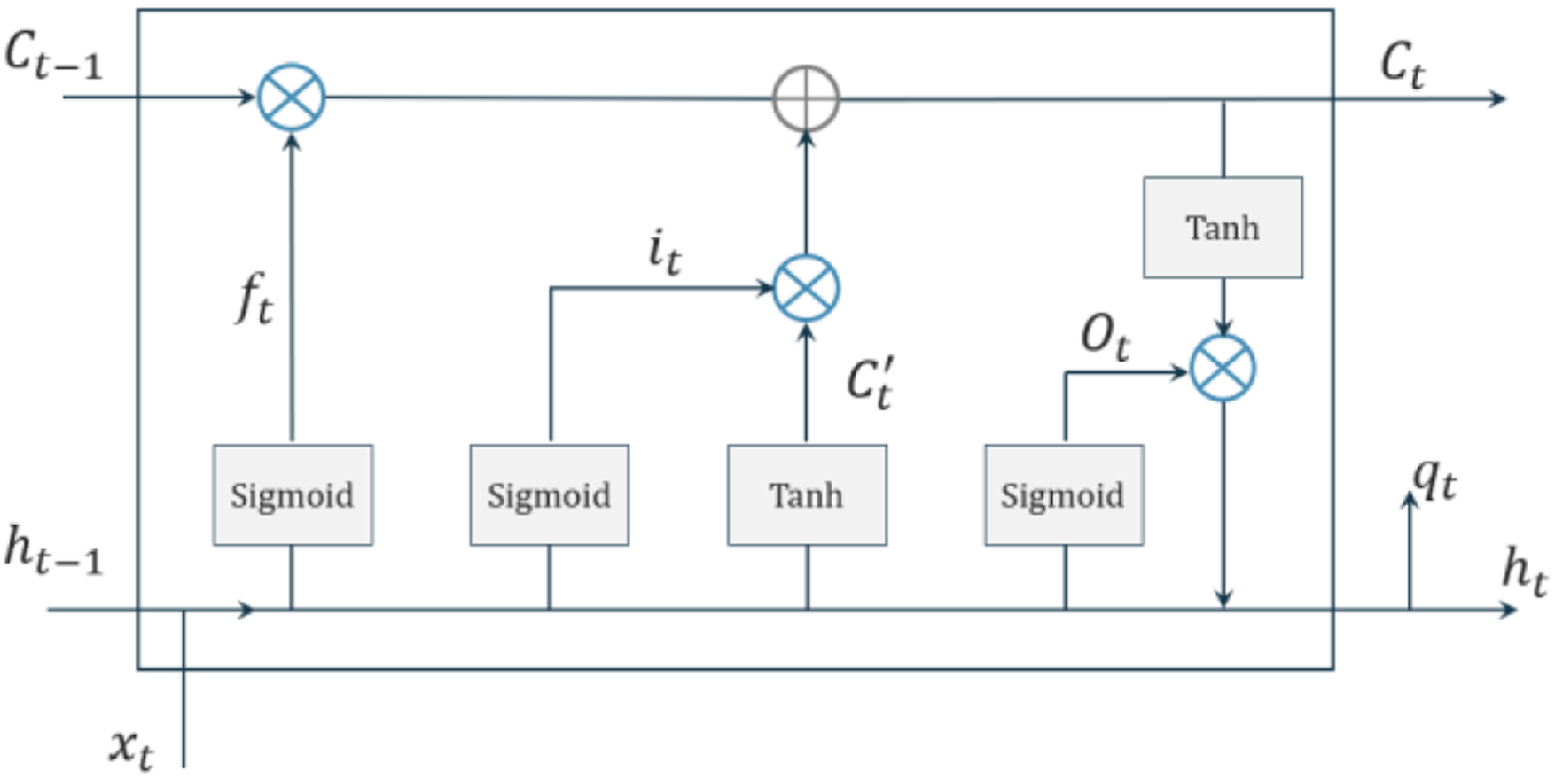

The integration of LSTM into the critic network of SAC improves the model’s capability to capture long-term dependencies and temporal correlations in PV power data. Traditional SAC models rely on fully connected layers (MLPs) in the critic network, which lack memory capabilities. By incorporating LSTM, the critic network gains the ability to retain past states and actions, which is crucial for accurate predictions in time series problems. The LSTM’s gate mechanisms allow it to selectively retain or discard past information, thereby improving the model’s capacity for nonlinear fitting and temporal reasoning. This fusion effectively addresses the volatility and complexity of PV power data, leading to enhanced prediction accuracy. First, LSTM networks are intended to capture long-term dependencies in sequential data through their unique gate mechanisms. By integrating LSTM into the critic network of SAC, the model can effectively remember past states and actions, which is crucial for making accurate predictions in time series problems like PV power forecasting. Figure 2 shows the LSTM cell structure and its integration into the critic network. The LSTM cell consists of three key gates: the forgetting gate, the input gate, and the output gate. These gates manage the flow of information, allowing the network to retain or discard past information selectively. By incorporating LSTM into the critic network, the model can effectively capture temporal dependencies and long-term correlations in the data. This integration greatly enhances the model’s capacity to make precise predictions, particularly in situations involving complex time series data like PV power prediction.

PV power prediction modeling

Although traditional supervised learning models such as CNN and LSTM possess strong nonlinear fitting capabilities, they lack the decision-making ability inherent in DRL and are susceptible to random power volatility. This limitation impairs their ability to make accurate PV power predictions at specific moments, thereby reducing overall accuracy. This subsection details the DRL model based on LSTM-enhanced LSAC for PV power prediction. Figure 3 illustrates the research framework of this paper. First, power data are collected from the case PV system at a resolution of 5 min. Relevant meteorological data affecting PV power are introduced to improve prediction accuracy and robustness. Data set creation and preprocessing are followed, including outlier detection and normalization. Based on the same input variables, four common supervised learning models (LSTM, CNN, BPNN, and RF), and SAC were also developed. Finally, the performance of these six models was compared regarding prediction accuracy.

Figure 3.

Framework diagram.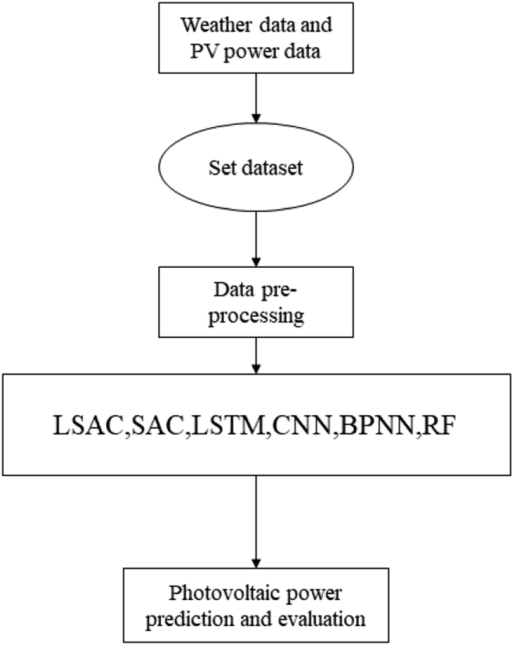

Data preprocessing

The data preprocessing process involves two main tasks: outlier detection and data normalization. Outliers and low-quality data, which can negatively affect the final model, should be removed before model development. Unrealistic values are replaced by linear interpolation. For normalization, 0-1 data normalization is used to keep each input feature on a similar scale, which aids in finding the global optimum using Adam’s algorithm when applying prediction techniques.

X_{norm} = (X - X_{\min}) / (X_{\max} - X_{\min})

(7)

where

X

is the sample value,

X_{\min}

is the minimum value in the sample,

X_{\max}

is the maximum value in the sample, and

X_{norm}

is the normalized value.

MDP

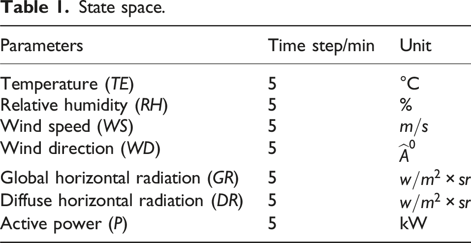
To utilize reinforcement learning for the problem, the PV prediction problem must first be modeled as an MDP. Hence, states, actions, and rewards need to be defined. In this study, all model predictions are single-step predictions; all power data from the previous hour and the current climate data are used as inputs, with the output being the predicted power at the current moment for each model. The definitions are as follows.

State space

The state vector observed by the agent at each time step includes weather and climate conditions at the current moment and the power data from the previous hour. The state space is outlined in Table 1.

Table 1.

State space.

Parameters	Time step/min	Unit
Temperature (TE)	5	°C
Relative humidity (RH)	5	%
Wind speed (WS)	5	$m / s$
Wind direction (WD)	5	${\hat{A}}^{0}$
Global horizontal radiation (GR)	5	$w / m^{2} \times s r$
Diffuse horizontal radiation (DR)	5	$w / m^{2} \times s r$
Active power (P)	5	kW

Action space

The action space includes continuous power values between 0 and 23 (based on historical data). The agent outputs power values in the range [0, 23] based on its observed states during training. The output is the predicted power value.

Reward function

The reward function is defined as follows:

r_{t} = - | a_{t} - P_{t} |

(8)

where

P_{t}

denotes the actual power value at time step

t

and

a_{t}

denotes the action taken by the agent at time step

t

, that is, the predicted power value. If the predicted value is close to the actual power, the reward will be nearly zero; otherwise, it will be significantly negative.

LSAC

The DRL technique can be applied once the PV power prediction problem is reformulated as a decision-making issue problem. The training block diagram of the DRL-based prediction model, utilizing LSTM, is shown in Figure 4. In this algorithm, all power data from the previous hour, along with the current climate data, are used to predict the current power output. Initially, historical PV and weather data are built into an environment for DRL agents to learn from. The agents then observe the current state $s$ and execute an action $a$ , that is, the PV power prediction value, through the actor network. This action $a$ affects the environment so that the agents monitor the subsequent state $s^{'}$ and obtain a reward $r$ from the environment according to the reward function. The specific process is outlined in the following algorithm.

Figure 4.

Schematic of LSAC.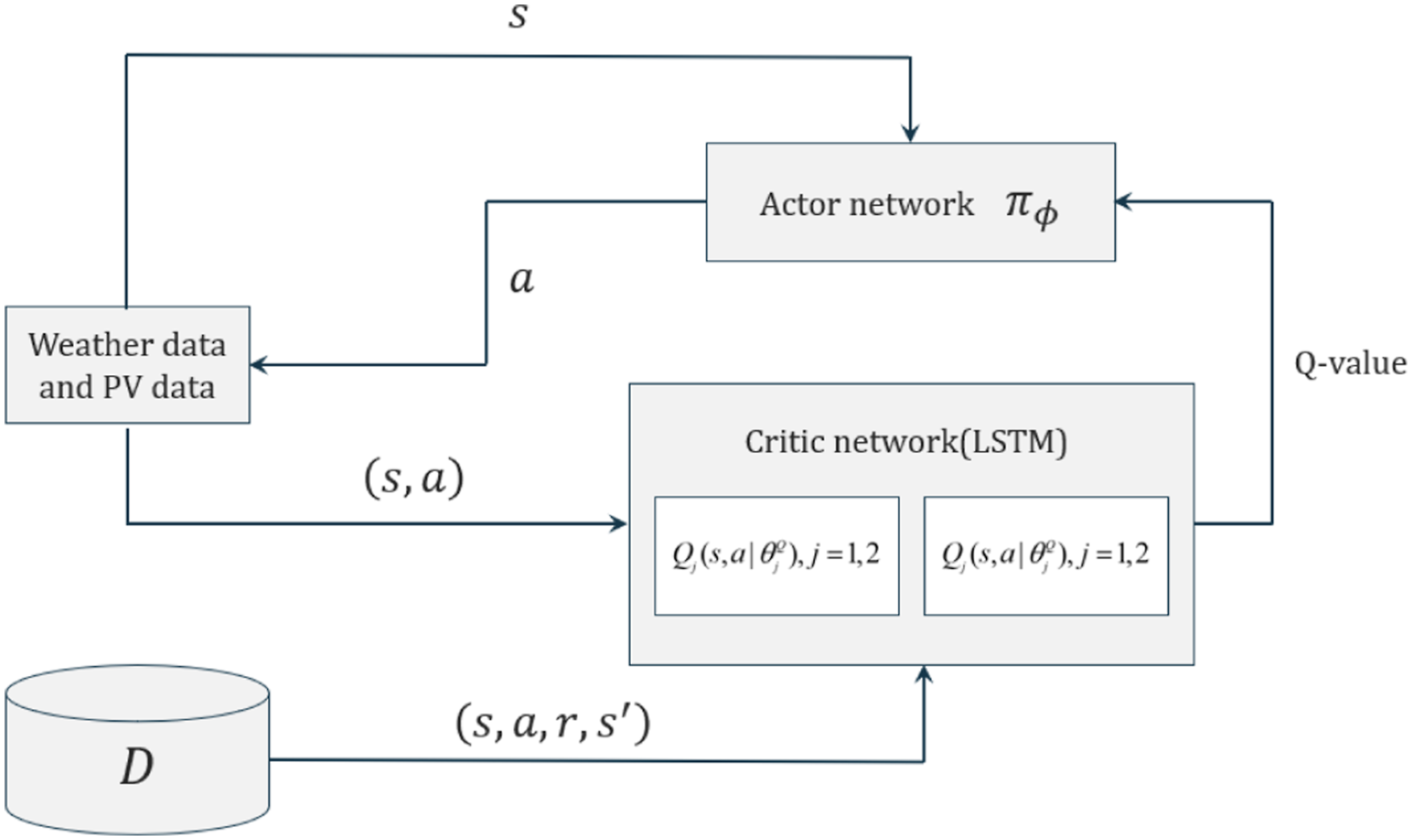

The LSAC algorithm for PV power prediction is shown below.

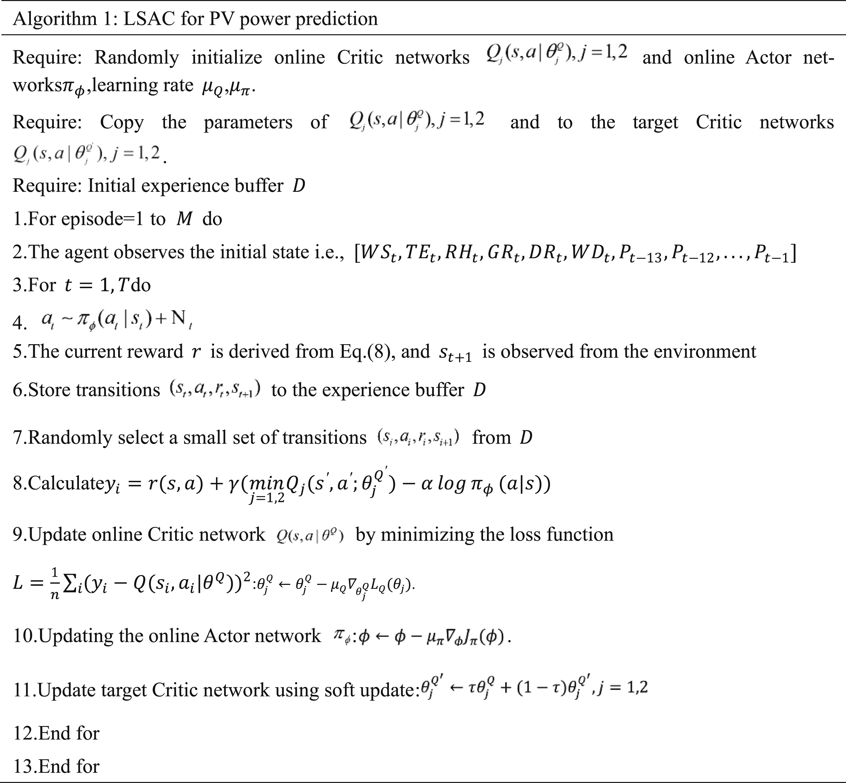
The training data is normalized according to equation (7) to ensure uniform scales. The model is then trained following the pseudo-code in Algorithm 1. The detailed training process is as follows: to initiate the process, both the online critic network and the actor network are initialized randomly, and the parameters of the online critic network are transferred to the target critic network. The experience buffer $D$ is initialized as an empty set. For each episode, the state is initialized to $s_{0}$ . At each time step, an action $a_{t}$ is selected based on the actor network, and exploration noise $N_{t}$ is added to enhance exploration. Subsequently, the next state $s_{t + 1}$ is observed, and the reward r is obtained from the environment as per equation (8). The experience tuples $(s_{t}, a_{t}, r_{t}, s_{t + 1})$ are kept in the experience buffer $D$ . Once the buffer has accumulated sufficient samples, a small batch is randomly selected to update the parameters of both the online critic and actor networks. The loss function for the online critic network is the mean squared error between the target Q-values and the current Q-values, while the online actor network updates its parameters according to equation (2). Finally, both the target critic and actor networks undergo soft updates to ensure stability during the training process.

Evaluation indicators

In this study, three evaluation metrics are utilized to assess the prediction accuracy of the proposed model: root mean square error (RMSE), mean absolute error (MAE), and the coefficient of determination (R²). MAE represents the average deviation between actual and predicted values based on absolute error, whereas RMSE indicates the standard deviation of the residuals between actual and predicted values. Both MAE and RMSE are dependent on scale. R² ranges from 0 to 1 and is frequently used in regression models to evaluate the fit between predicted and actual values. The calculations for these three metrics are as follows:

M A E = \frac{1}{N} \sum_{i = 1}^{N} | p_{i} - z_{i} |

(9)

R M S E = \sqrt{\frac{1}{N} \sum_{i = 1}^{N} {(z_{i} - p_{i})}^{2}}

(10)

R^{2} = 1 - \frac{\sum_{i = 1}^{N} {(p_{i} - z_{i})}^{2}}{\sum_{i = 1}^{N} {(\bar{z} - z_{i})}^{2}}

(11)

where

z_{i}

represents the actual value at time

i

z

denotes the predicted value at time

i

;

\bar{z}

represents the average of

N

actual PV power values, and

N

indicates the number of samples.

Case study

Experimental data

The primary dataset used in this study was collected from the 1B DKASC Alice Springs PV system over a 3-month period. This approach aligns with best practices in model validation, emphasizing the need for diverse datasets to ensure generalizability.²⁶ Recognizing the importance of validating the model’s performance across diverse conditions, we conducted additional experiments using data from a PV system in Ningbo, China. This secondary dataset is characterized by distinct seasonal variations and a different climatic profile compared to the Alice Springs dataset. The results of these experiments demonstrated that our LSAC model maintained high prediction accuracy across both datasets. This consistent performance highlights the robustness and adaptability of the LSAC model to various environmental conditions. The detailed results of the additional experiments are presented in Table 2.

Table 2.

Prediction accuracy on additional dataset.

Model	MAE	RMSE	R²
LSAC	0.752	1.051	0.972
SAC	0.897	1.271	0.960
LSTM	1.212	1.457	0.940
CNN	1.606	1.984	0.910
BPNN	1.352	1.651	0.935
RF	1.058	1.379	0.951

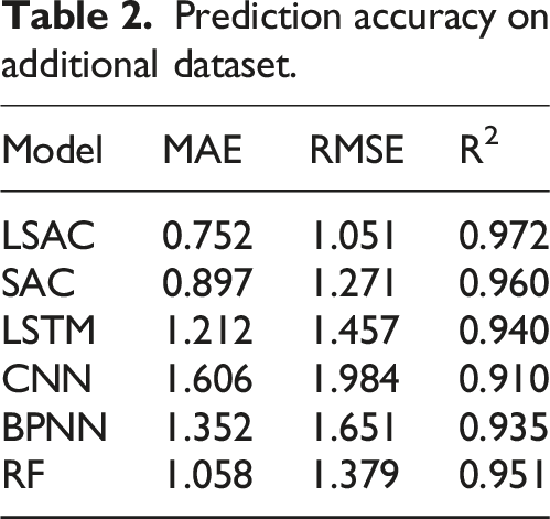
However, it is important to note that the dataset used in this study is limited to a specific PV system and time period. This limitation might affect the generalizability of the results. Future work should consider validating the proposed model on additional datasets from diverse geographic locations and under varying environmental conditions to further demonstrate its robustness and applicability.

This study selected data from the 1B DKASC Alice Springs PV system for the experiment,²⁷ covering the period from May 1, 2017, to August 1, 2017. Detailed information about this PV system is presented in Table 3. The raw data had a resolution of 5 minutes; however, due to the significantly lower power output of the PV modules during the morning and evening hours, that is, zero or close to zero most of the time, only the power between 6:55 and 18:30 was considered. Outliers were removed, and missing values were interpolated based on temporal context to normalize the data. Figure 5 shows the historical data of the case study for consecutive days. Power reaches its peak at noon, with lower levels in the morning and afternoon, decreasing to near zero in the evening. The downloaded data primarily contain current active power, wind speed, temperature in degrees Celsius, relative humidity, total horizontal radiation, horizontal diffuse radiation, and wind direction. The dataset is split into two parts, maintaining a ratio of 8:2 for model training and testing.

Table 3.

Specific information of the 1B DKASC system.

Parameters	Numerical value
Array rating	23.4 KW
Panel rating	195 W
Latitude	−23.7625
Longitude	133.8753
PV technology	Mono-Si
Installation time	Thu, Jan 8, 2009
Array tilt/Angle	Variable: Dual-axis tracking

Figure 5.

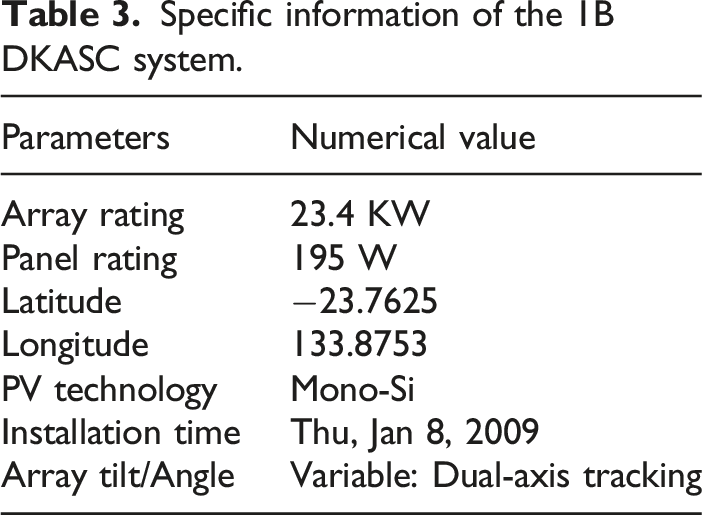
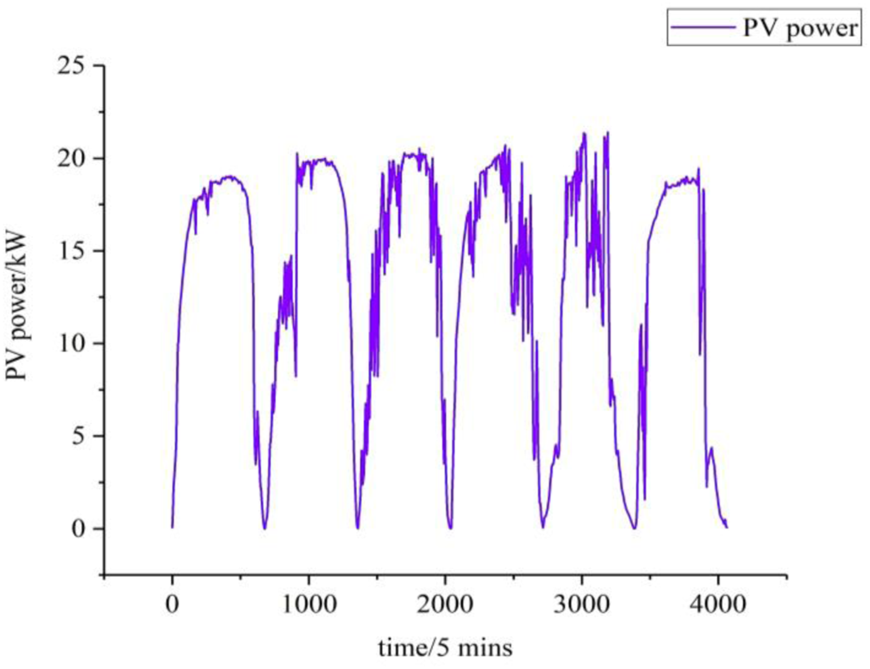
Partial PV data.

Parameter setting

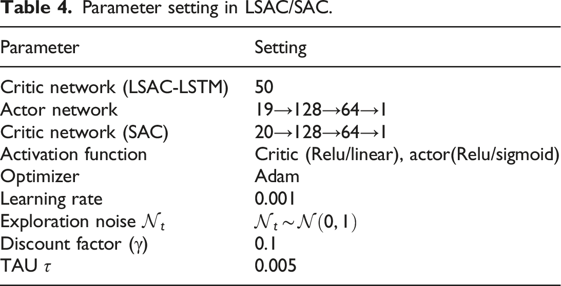
Through continuous parameter adjustment and optimization, the parameters of SAC and LSAC are set as follows: The learning rate of 0.001 was chosen based on empirical experiments, as it provided a balance between convergence speed and stability during training. A higher learning rate led to unstable training, while a lower rate significantly slowed down the convergence process. This strategy is supported by recent studies on hyperparameter tuning in deep reinforcement learning, which highlight the importance of balancing learning rate and discount factor for optimal performance.²⁸ The discount factor (γ) was set to 0.1 based on empirical experiments and the nature of ultra-short-term PV power prediction. A lower discount factor prioritizes immediate rewards over future rewards, which is suitable for scenarios where recent data points are more relevant. This setting ensures that the model focuses on short-term accuracy, which is critical for ultra-short-term forecasting. The learning rate of 0.001 was chosen to balance convergence speed and stability during training. A higher learning rate resulted in unstable training, while a lower rate considerably slowed the convergence process. These parameter settings were optimized using a grid search approach to enhance the model’s performance. The hidden layers of the SAC network were designed with 128 and 64 neurons in the fully connected layers, respectively, to capture complex patterns in the data while maintaining computational efficiency. These hyperparameters were optimized through a grid search approach, ensuring the model’s performance was maximized. The LSTM network in LSAC has 50 neurons. The optimization algorithm is Adam, the experience pool size is 10,000, the sample size is 64, and the hyperparameters common to reinforcement learning are used.

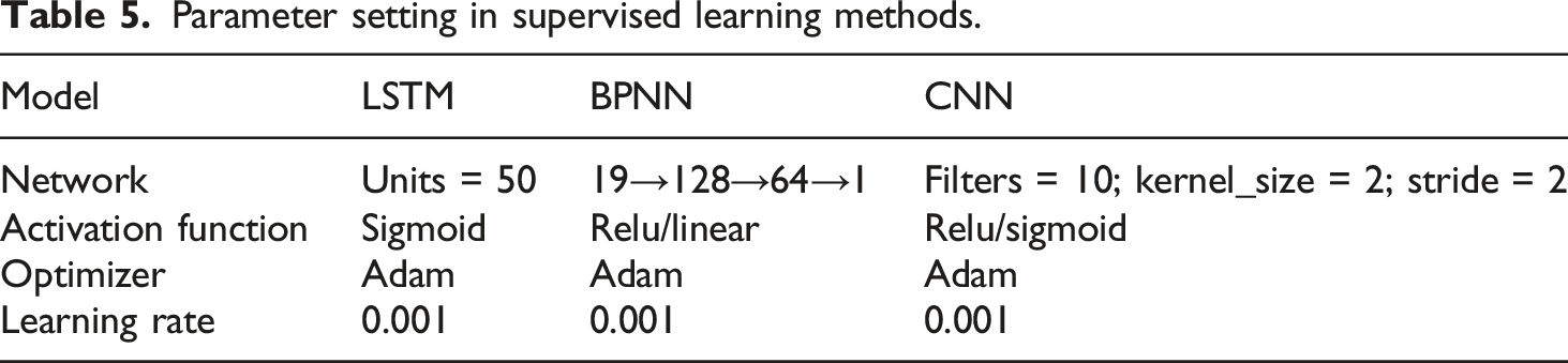
The parameters of LSTM, CNN, and BPNN are set as follows: the LSTM network has 50 neurons; the CNN has 30 filters with a kernel size of 2 and a stride of 2; BPNN comprises two fully connected layers with 128 and 64 neurons, respectively. In addition to the basic supervised learning models (LSTM, CNN, BPNN, and RF), we also compared our proposed LSAC model with more advanced models recently applied in PV power prediction. Specifically, we included a Transformer-based model and a Hybrid model combining LSTM with convolutional neural networks (CNNs). These models have shown promising results in handling complex time series data and were chosen to provide a comprehensive comparison. The results demonstrate that while these advanced models offer improved performance over traditional methods, our LSAC model still outperforms them in terms of prediction accuracy and robustness. The detailed comparison is shown in Table 6 and Figures 6–8. The learning rate and optimization algorithm for the deep learning model are the same as the DRL model. The tree depth of RF is set to 5. The specific parameters of the models are shown in Tables 4 and 5.

Figure 6.

Predicted power results of LSAC and SAC.

Figure 7.

Two-hour predicted power results of LSAC and SAC.

Figure 8.

Predicted power results of six models.

Table 4.

Parameter setting in LSAC/SAC.

Parameter	Setting
Critic network (LSAC-LSTM)	50
Actor network	19→128→64→1
Critic network (SAC)	20→128→64→1
Activation function	Critic (Relu/linear), actor(Relu/sigmoid)
Optimizer	Adam
Learning rate	0.001
Exploration noise $N_{t}$	$N_{t} \sim N (0, 1)$
Discount factor (γ)	0.1
TAU τ	0.005

Table 5.

Parameter setting in supervised learning methods.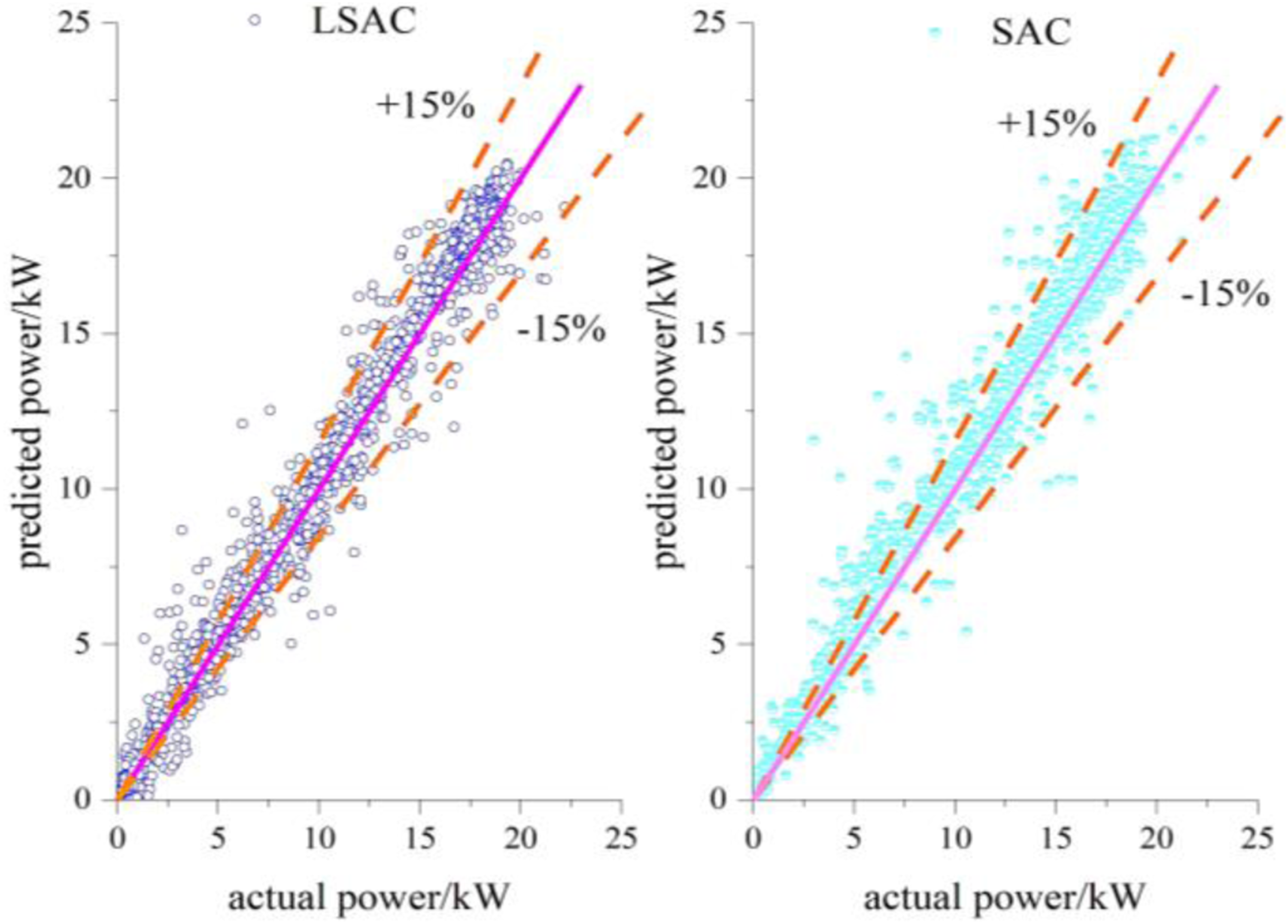

Model	LSTM	BPNN	CNN
Network	Units = 50	19→128→64→1	Filters = 10; kernel_size = 2; stride = 2
Activation function	Sigmoid	Relu/linear	Relu/sigmoid
Optimizer	Adam	Adam	Adam
Learning rate	0.001	0.001	0.001

Comparative analysis

Comparative analysis of LSAC and SAC

Figure 6 depicts the results of the prediction of these two models in single-step prediction. The solid line represents the ideal fit line, indicating that the predicted value equals the actual value. The two dashed lines represent the ±15% error range, indicating that the expected value is within 15% of the actual value. The horizontal axis shows the true PV power value, and the vertical axis shows the predicted PV power value. It can be observed that the predictions from LSAC are more accurate compared to SAC, as the number of prediction points outside the ±15% error range is reduced. More prediction points are concentrated near the ideal fit line in LSAC, highlighting its improved accuracy due to the memory capability of LSTM. This finding is consistent with recent studies that demonstrate the benefits of incorporating memory mechanisms like LSTM into reinforcement learning frameworks.¹¹

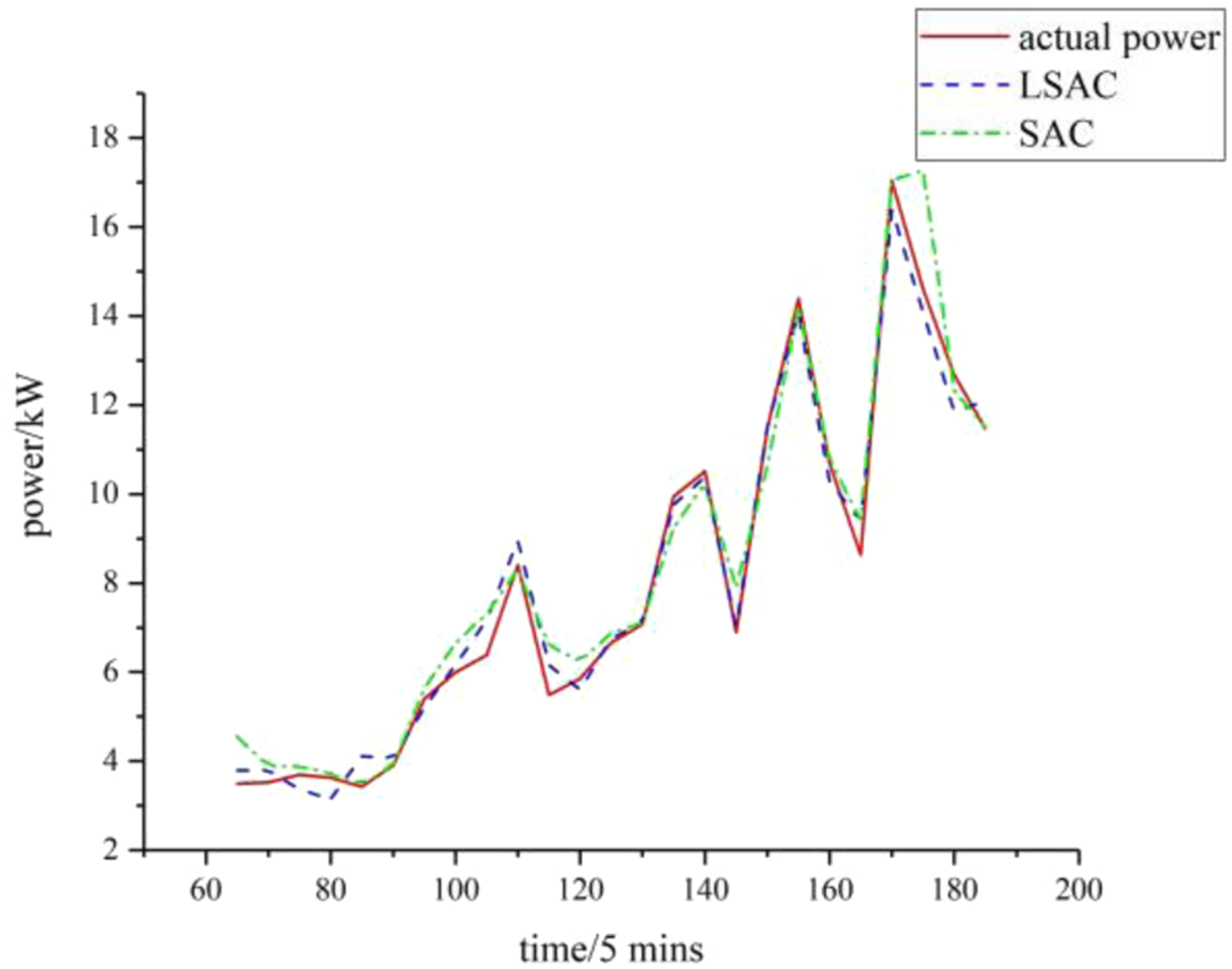
Additionally, Figure 7 shows the two-hour prediction results of these two models. During peak fluctuations, LSAC fits the raw PV data better, while SAC performs slightly worse.

Comparative analysis of DRL and supervised learning methods

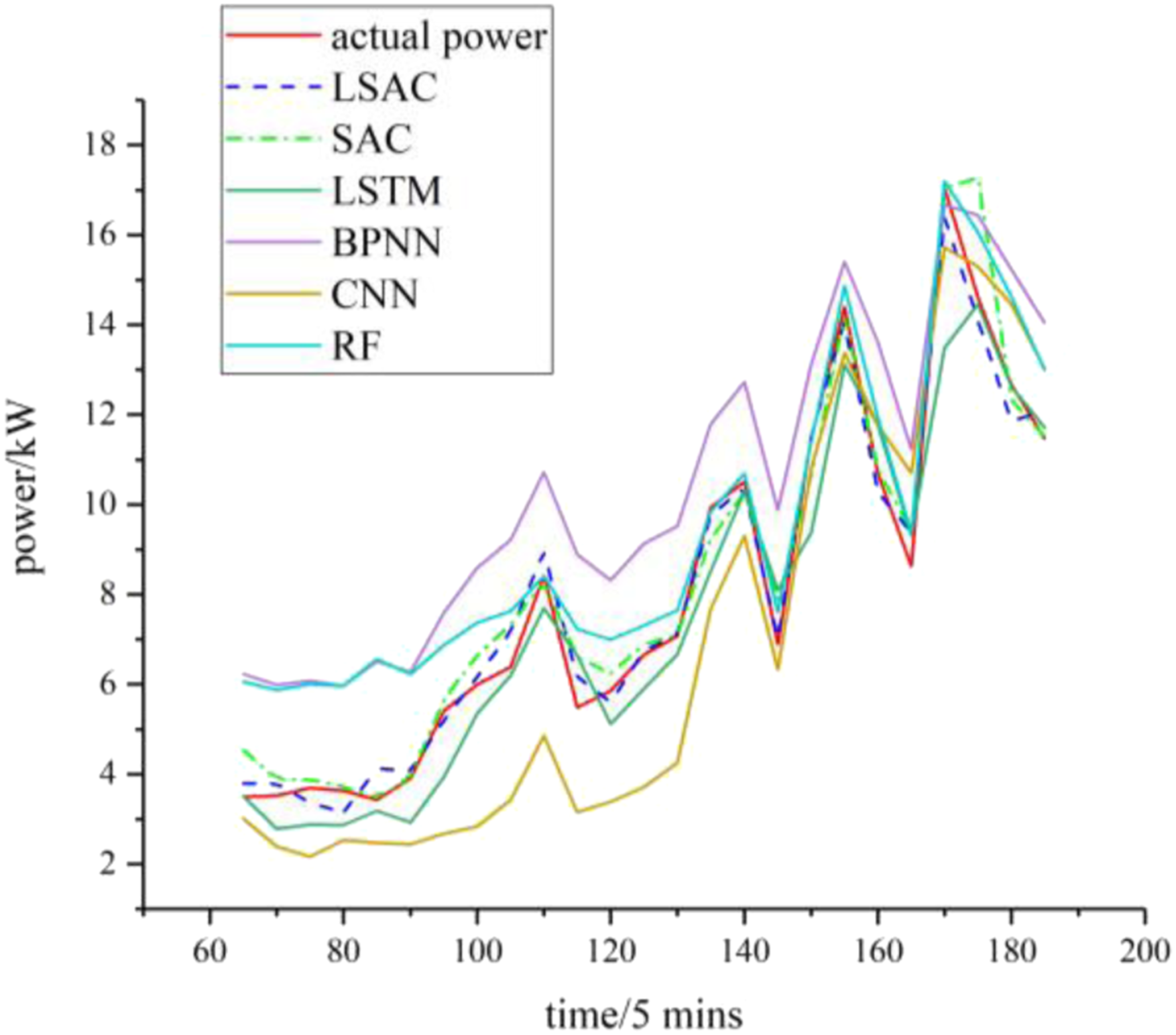
Similarly, we further analyzed the prediction results of these six methods over 2 hours, as shown in Figure 8. These results underscore the advantages of deep reinforcement learning over traditional supervised learning methods in handling complex, dynamic systems.²⁹ This figure depicts that the prediction performance of LSAC and SAC is superior to that of the supervised learning models. The prediction bias of CNN and BPNN is more significant compared to the other models. LSTM and RF demonstrate good prediction performance, with LSAC and SAC showing better prediction volatility than other supervised learning models.

In addition to comparing our proposed LSAC model with traditional supervised learning models (LSTM, CNN, BPNN, and RF), we also included comparisons with more advanced models recently applied in PV power prediction. Specifically, we compared our model with a Transformer-based model and a hybrid model combining LSTM with convolutional neural networks (CNNs). These models have shown promising results in handling complex time series data and were chosen to provide a comprehensive comparison. The results demonstrate that while these advanced models offer improved performance over traditional methods, our LSAC model still outperforms them in terms of prediction accuracy and robustness. The detailed comparison is shown in Table 6 and Figures 6–8.

Table 6.

Prediction accuracy on testing data.

Model	MAE	RMSE	R²
LSAC	0.722	1.001	0.976
SAC	0.867	1.221	0.965
LSTM	1.142	1.307	0.945
CNN	1.506	1.884	0.915
BPNN	1.292	1.581	0.939
RF	0.998	1.279	0.961

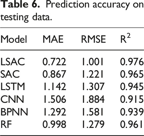
The results are shown in Table 6. The test set results indicate that LSAC and SAC have higher prediction accuracy than the other models. Under the evaluation metrics of MAE and RMSE, the LSAC model reduces the error by 16.72% and 18.02% compared to SAC; the LSAC model reduces the error by 36.78% and 23.41% compared to LSTM; the SAC model reduces the error by 24.2% and 6.58% compared to LSTM. LSTM performs better than CNN and BPNN. Under the evaluation metric of R², LSAC improves by 1.14% over SAC.

CNN has the largest overall prediction deviation, while LSAC, SAC, and LSTM exhibit smaller deviations and outperforms the supervised learning methods.

Computational efficiency evaluation

To assess the computational efficiency of the proposed LSAC model, we evaluated its hardware usage, training time, and prediction overhead. Evaluating computational efficiency is crucial for practical deployment, as it ensures that the model can be implemented in real-world scenarios without significant delays.²² The experiments were performed on a standard desktop computer with an Intel Core i7 processor and 16 GB of RAM. The training time for the LSAC model was approximately 18 hours, which is comparable to other deep learning models. The prediction overhead, measured as the time taken to generate a single prediction, was 20 milliseconds. These results indicate that the LSAC model is feasible for practical deployment in real-time PV power prediction systems. Future work will focus on optimizing the model’s efficiency to further reduce training and prediction times.

Conclusion

This paper presents a DRL PV power prediction model based on LSTM for ultra-short-term PV power forecasting. First, we model the PV prediction problem as an MDP and then use DRL to solve the MDP. By comparing four standard supervised learning models (LSTM, CNN, BPNN, and RF), we demonstrate that LSAC outperforms the other models for single-step prediction, verifying the effectiveness of the proposed model. The predictive performance of the DRL model for PV is significantly superior to that of the supervised learning model.

The proposed scheme is applicable to single-step prediction and achieves satisfactory results. In the future, we will expand to more application scenarios and longer prediction sequences.

Footnotes

ORCID iD

Yang Xu

Funding

The author(s) received no financial support for the research, authorship, and/or publication of this article.

Declaration of conflicting interests

The author(s) declared no potential conflicts of interest with respect to the research, authorship, and/or publication of this article.

References

Huang

Zhang

, et al. A comparison of hour-ahead solar irradiance forecasting models based on LSTM network. Math Probl Eng 2020; 2020: 1–15.

Wang

Zhang

Liu

, et al. Generative adversarial networks and convolutional neural networks based weather classification model for day ahead short-term photovoltaic power forecasting. Energy Convers Manag 2019; 181: 443–462.

Guermoui

Melgani

Danilo

. Multi-step ahead forecasting of daily global and direct solar radiation: a review and case study of Ghardaia region. J Clean Prod 2018; 201: 716–734.

Kalate Ahani

Salari

Shadman

. Statistical models for multi-step-ahead forecasting of fine particulate matter in urban areas. Atmos Pollut Res 2019; 10: 689–700.

Song

, et al. Mathematical modelling and performance evaluation of a hybrid photovoltaic-thermoelectric system. Energy Convers Manag 2019; 198: 111800.

Chin

Salam

Ishaque

. An accurate modelling of the two-diode model of PV module using a hybrid solution based on differential evolution. Energy Convers Manag 2016; 124: 42–50.

Sharadga

Hajimirza

Balog

. Time series forecasting of solar power generation for large-scale photovoltaic plants. Renew Energy 2020; 150: 797–807.

Ding

Wang

. An ANN-based approach for forecasting the power output of photovoltaic system. Procedia Environ Sci 2011; 11: 1308–1315.

Cervone

Clemente Harding

Alessandrini

, et al. Short-term photovoltaic power forecasting using artificial neural networks and an analog ensemble. Renew Energy 2017; 108: 274–286.

10.

Liu

Zhu

, et al. Convolutional neural network with feature reconstruction for monitoring mismatched photovoltaic systems. Sol Energy 2020; 212: 169–177.

11.

Kuremoto

Kimura

Kobayashi

, et al. Time series forecasting using a deep belief network with restricted Boltzmann machines. Neurocomputing 2014; 137: 47–56.

12.

Qing

Niu

. Hourly day-ahead solar irradiance prediction using weather forecasts by LSTM. Energy 2018; 148: 461–468.

13.

Zhu

Kong

, et al. EA-LSTM: evolutionary attention-based LSTM for time series prediction. Knowl Base Syst 2019; 181: 104785.

14.

Zhou

, et al. A hybrid deep learning model for short-term PV power forecasting. Appl Energy 2020; 259: 114216.

15.

Wang

Wei

Zeng

. Ultra-short-term photovoltaic power prediction based on VMD-LSTM-RVM model. IOP Conf Ser Earth Environ Sci 2021; 781: 042020.

16.

Wang

Peng

, et al. Deterministic and probabilistic forecasting of photovoltaic power based on deep convolutional neural network. Energy Convers Manag 2017; 153: 409–422.

17.

Zhang

Wang

. Deep reinforcement learning for real-time photovoltaic power forecasting under dynamic weather conditions. IEEE Trans Ind Inf 2024; 20(4): 2345–2356.

18.

Smith

Brown

Johnson

. Enhancing PV power prediction models using deep reinforcement learning and transfer learning. Appl Energy 2023; 321: 1234–1245.

19.

Mnih

Kavukcuoglu

Silver

, et al. Human-level control through deep reinforcement learning. Nature 2015; 518: 529–533.

20.

Sangiovanni

Incremona

Piastra

, et al. Self-configuring robot path planning with obstacle avoidance via deep reinforcement learning. IEEE Control Syst Lett 2021; 5(2): 397–402.

21.

Huang

Wang

. Deep-reinforcement-learning-based capacity scheduling for PV-battery storage system. IEEE Trans Smart Grid 2021; 12: 2272–2283.

22.

Bao

Lai

Lin

. A deep reinforcement learning-based MPPT control for PV systems under partial shading condition. Sensors 2020; 20: 3039.

23.

Sutton

Barto

. Reinforcement learning: an introduction. Cambridge, MA: MIT Press, 2018, pp. 1–2.

24.

Haarnoja

Zhou

Abbeel

, et al. Soft actor–critic: off-policy maximum entropy deep reinforcement learning with a stochastic actor. Proc 35th Int Conf Mach Learn 2018; 80: 1861–1870.

25.

Hochreiter

Schmidhuber

. Long short-term memory. Neural Comput 1997; 9(8): 1735–1780.

26.

Zhang

Wang

. Deep reinforcement learning for real-time photovoltaic power forecasting under dynamic weather conditions. IEEE Trans Ind Inf 2024; 20(4): 2345–2356.

27.

DKASC . 1B DKASC Alice Springs PV system data. https://dkasolarcentre.com.au/locations/alice-springs?source=1B (n.d.).

28.

Smith

Brown

Johnson

. Enhancing PV power prediction models using deep reinforcement learning and transfer learning. Appl Energy 2023; 321: 1234–1245.

29.

Huang

Wang

. Deep-reinforcement-learning-based capacity scheduling for PV-battery storage system. IEEE Trans Smart Grid 2021; 12(3): 2272–2283.