Dynamic strategy research on “following speed—safety distance” for autonomous driving

Abstract

Based on a simulation testing platform, the correlation between the main vehicle’s following speed, following distance, and other parameters under sudden traffic conditions is analyzed. An experimental scenario of “front vehicle stationary, preceding vehicle suddenly cutting out, and main vehicle decelerating to avoid collision” is designed. Through the collection and analysis of experimental data, the data in the simulation process is tracked, and the response performance of the main vehicle under different parameter conditions is evaluated. Latin hypercube sampling generalization tests are used to further explore and verify the applicability of the findings. The research indicates that the following speed and following distance exhibit a quadratic function relationship. Reasonably optimized following speed and following distance can significantly enhance vehicle driving safety.

Keywords

autonomous driving simulation testing following safety Latin hypercube sampling

Introduction

With the rapid development of autonomous driving technology, the safety and reliability of vehicles in complex traffic environments have attracted widespread attention.¹ Closed-road and open-road tests for vehicle safety face issues such as high testing costs and a lack of extreme testing scenarios.² Simulation testing can accurately describe the dynamic relationship between autonomous vehicles and various components of the driving environment under specific driving tasks over a period of time.³ It allows for extensive virtual testing before actual vehicle testing and can detect the response capability⁴ and decision-making strategies⁵ of the system and vehicle, effectively verifying intelligent driving functions.⁶

The research experiment refers to Appendix A.5 of the i-vista2023 test procedure,⁷ and designs an experimental scenario of “front vehicle stationary, preceding vehicle suddenly cutting out, and main vehicle decelerating to avoid collision.” It aims to simulate typical sudden traffic situations and analyze the driving conditions of the main vehicle under different following speeds and following distances. Through the collection and analysis of experimental data, the relationship between parameters such as speed and distance is explored, and data generalization techniques are used to verify the applicability of the experimental conclusions.

Introduction to the autonomous driving simulation platform

Autonomous driving simulation testing

Ensuring driving safety of autonomous vehicles in sudden events, adverse weather, and extreme road conditions has become a critical issue in autonomous driving technology.⁸ To prove that an autonomous driving system is safe, theoretically, a vast number of scenarios need to be tested to fully demonstrate the system’s safety.⁹ The core of simulation testing lies in the ability to simulate various driving scenarios and emergencies by building virtual scenes and vehicle models without the need for real vehicles or roads.¹⁰ It not only reduces costs and safety risks but also provides feasibility for large-scale experiments. Through a high-fidelity simulation platform, developers can comprehensively test the perception, decision-making, and control modules of the autonomous driving system, providing key data support for its optimization and upgrading.¹¹

VTD simulation software

Virtual Test Drive (VTD) is a vehicle simulation software developed by the German company VIRES, used for the development and testing of autonomous driving systems. VTD provides a customizable virtual environment that can accurately simulate various traffic conditions. Its core functions include constructing static/dynamic scenes, using vehicle dynamics simulation models for vehicle driving and environment interaction, and integrating with external systems for joint simulation.¹² Specifically, it can generate or read odr road information files, osgb image data files, xml/xosc dynamic scene files, interface with third-party software and functional plugins, and generate parameter data during the simulation process.

Simulation platform overview

The architecture of the simulation platform used in this research experiment is shown in Figure 1. The operation of the platform mainly consists of three steps: First, based on the scenario library, suitable test scenarios are selected, and the initial conditions of the simulation, such as the initial vehicle position, are defined. Then, the vehicle model, dynamics model, driver model, and the algorithm under test (integrated with the Carlink collaborative control framework) are selected, and the VTD simulation software is invoked to achieve multi-module interaction and simulation. After the simulation ends, the required target data, such as the state parameters of the tested vehicle, are selected and extracted from the test database for subsequent analysis and performance evaluation.

Figure 1.

Simulation platform architecture.

As the core component of the algorithm under test, Carlink enables real-time data interaction between the algorithm module, vehicle model, and Trigger instructions during the simulation process, supporting multi-protocol and multi-configuration compatibility. Through the built-in state machine management module, it monitors experimental parameters and dynamically adjusts various parameters during the simulation. The timestamp function is utilized to coordinate the VTD simulation step size with the algorithm decision-making cycle, reducing timing mismatch errors.

In this experiment, to minimize the interference of sensors on the experimental results, the sensor model is not used. A test experiment is conducted to anchor the parameter configuration, and the vehicle is fully controlled through the algorithm and Trigger.

Generalization method: Latin hypercube sampling

Latin Hypercube Sampling (LHS) is a statistically efficient sampling method widely used for high-dimensional space sampling strategies. It effectively performs uniform spatial sampling of multiple variables by dividing the range of each variable into multiple intervals and selecting a sample point within each interval, ensuring a uniform distribution of samples.¹³

For each dimension j∈[1,d] in a d-dimensional space, the domain of each dimension j is first divided into n equal-width subintervals, with the interval width denoted as interval_size[j]. Then, according to the order of each dimension j, a random permutation Pj of length n is generated. Each sample point Pj[i] (1 ≤ i ≤ n) undergoes uniform random sampling within its corresponding subinterval. Finally, the sampling results of each dimension are arranged and combined to form an n × d sample matrix, where the ith sample data can be represented as {P1[i], P2[i]…Pj[i]…Pd[i]}.¹⁴

The Latin hypercube sampling pseudocode will be presented below, and sampling will be demonstrated using two methods: normalization and obtaining specific sample data:

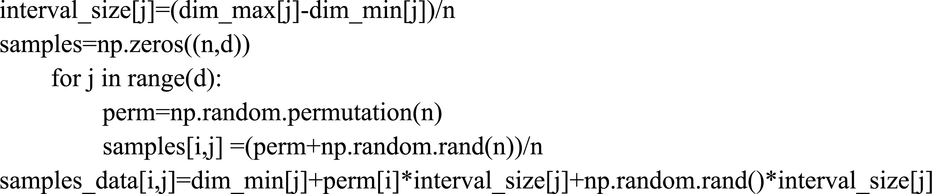
Latin hypercube sampling has the following advantages: It uniformly covers the entire space, ensuring that the entire interval of each dimension is adequately represented. It effectively reduces the occurrence of redundant data points, improves sampling efficiency, and reduces the number of sampling points. It guarantees the unbiasedness of each dimension, and the sampling results have high representativeness.¹⁵

Scenario and experimental design

Simulation scenario design

The content of this experiment is “front vehicle stationary, preceding vehicle suddenly cutting out, and main vehicle decelerating to avoid collision.” To achieve this goal, it is necessary to design the corresponding Opendrive static map and Scenario dynamic settings based on this content.

In the design of the Opendrive static map, the length of all the vehicles is 4.674 m, the experiment prepares a three-lane road with a length of at least 1 km, and the width of each motor vehicle lane is 3.75 m, providing the preceding vehicle with the necessary driving space for cutting out of the current lane. Additionally, to avoid interference from other environmental factors in the experimental scenario, the overall structure of the road is set as a straight line and configured as a one-way driving section without intersections, ensuring that the driving behavior of the main vehicle and the preceding vehicle are the primary focus of the experiment.

In the design of the Scenario dynamic settings, it is necessary to simulate the time required for the main vehicle to identify the stationary front vehicle after the preceding vehicle cuts out. At the same time, to reduce the interference of sensor errors on the experimental results, a relatively fixed trigger moment is set for the deceleration event of the main vehicle. Specifically, the experiment takes the time point when the preceding vehicle completely leaves the center line of the current lane as the trigger moment for the main vehicle’s braking, as shown in Figure 2, Ego represents the main test vehicle, which needs to successfully brake without colliding with the front vehicle. VT1 is the preceding vehicle that cuts out, and VT2 is the stationary target vehicle in front. This design provides a stable trigger condition when the lane change time of the preceding vehicle remains unchanged, while realistically simulating the scenario where the main vehicle observes the stationary front vehicle and performs an avoidance response.

Figure 2.

Experimental scenario diagram.

Experimental procedure and data collection

Data collection is the core part of this experiment. All experimental data is collected in real-time through the built-in data tracking and recording function of the simulation platform. The required vehicle coordinate information is selected to generate CSV files for data storage. To comprehensively evaluate performance, we collect various data, including but not limited to vehicle position, speed, and acceleration, from which we can derive other indicators such as distance between vehicles and whether a collision has occurred.

We first perform a small test experiment, focusing on collecting data when the experimental vehicle performs a rapid lane change at a test condition of v = 60 km/h and TTC_{TV1_TV2} = 1.5 s. We calculate the time point when the vehicle completely leaves the center line of the current lane, determining the time point to control the main vehicle’s braking in the basic experiment, to better simulate the main vehicle’s actual identification and response process to the front vehicle.

After obtaining the results of the test experiment, we set up subsequent experiments based on the test results. The specific process is shown in Figure 3:

Figure 3.

Basic experimental flowchart.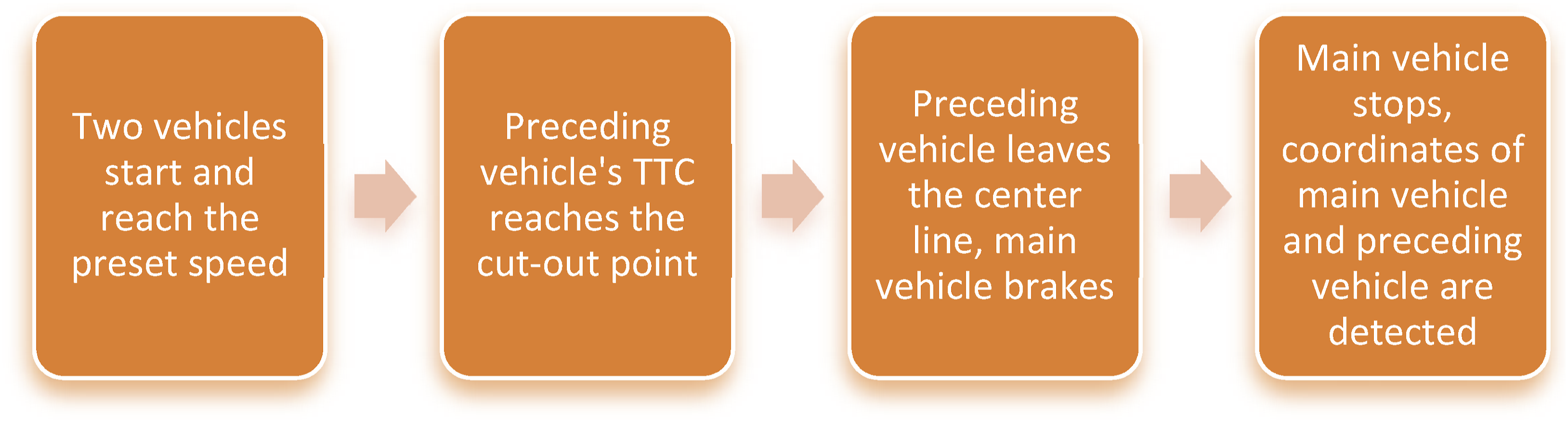

After the experimental data is collected in real-time through the VTD platform, all data is recorded as CSV files, and we need to conduct in-depth analysis of this data. First, the most important indicator is whether a collision occurs between the main vehicle and the stationary front vehicle. Collision detection is based on the distance between the main vehicle and the front vehicle. When the distance between the two vehicles is less than the set safety distance, it is determined that a collision has occurred.

On the basis of collision detection, to assess whether the main vehicle can effectively avoid the preceding vehicle, we further analyze the distance between the vehicles after braking and calculate the minimum distance between the main vehicle and the preceding vehicle. Additionally, we calculate the theoretical remaining distance, which is the distance theoretically remaining between the main vehicle and the front vehicle after the main vehicle brakes while traveling with the current data. This is used for theoretical analysis of the data and to determine the accuracy of the simulation. A smaller value of the theoretical remaining distance indicates a higher risk of collision between the main vehicle and the front vehicle, while a larger theoretical remaining distance indicates a greater margin for reaction in potential collision scenarios. Through these indicators, we can quantitatively evaluate the safety margin in sudden traffic situations.

Basic experiment

In the basic scenario, the parameter settings for the main vehicle, preceding vehicle, and front vehicle are shown in Table.1. These parameter settings refer to the “Intelligent Driving Index—Evaluation Regulations for Navigation Intelligent Driving System (Urban Roads).” The main vehicle and the preceding vehicle both travel at a speed of 60 km/h, with a distance of 25 m between them. The Time to Collision (TTC) between the preceding vehicle and the front vehicle, which is the remaining time before a collision is expected to occur under the current relative speed (Δv) and distance (Δd) conditions, is calculated as TTC = |Δd/Δv|, Δv≠0. When the TTC of the preceding vehicle decreases to 1.5 s, the autonomous driving system triggers an emergency lane change operation. The main vehicle brakes with an acceleration of 5 m/s², while the front vehicle remains stationary, conforming to the general speed requirements in urban scenarios. Additionally, the experiment selects an ordinary passenger vehicle as the simulation vehicle to reduce the influence of external variables on the experimental results and to investigate the general situation in common scenarios.

Table 1.

Basic scenario parameter settings.

Main vehicle speed V_Ego (km/h)	Distance between main vehicle and preceding vehicle L_{Ego_TV1}(m)	Time to collision between preceding vehicle and front vehicle TTC_{TV1_TV2}(s)	Main vehicle braking acceleration A_Ego (m/s²)	Vehicle type (TV1, TV2, TV3)
60	25	1.5	5	Passenger car

Through the above dynamic settings, the experiment effectively simulates the sudden traffic situation, accurately reproducing the scenario where the front vehicle is stationary, the preceding vehicle suddenly cuts out, and the main vehicle decelerates to avoid a collision. It also provides relatively precise trigger conditions and controllable initial states for analyzing the deceleration avoidance behavior of the main vehicle.

Controlled variable experiment

To further verify the experimental results and investigate the relationship and influence between parameters such as following speed and following distance, this experiment adopts the controlled variable method and designs various experimental scenarios, as shown in Table.2, covering different initial vehicle speeds, following distances, and lane change times of the preceding vehicle. This ensures that experimental results have high applicability and stability, providing a reliable theoretical basis.

Table 2.

Generalization parameter settings.

V_Ego (km/h)	L_{Ego_TV1} (m)	TTC_{TV1_TV2} (s)	A_Ego (m/s²)	Target object type
60	15	1.5	5	Passenger car
60	25	1.2	5	Passenger car
60	25	1.5	4	Passenger car
80	25	1.5	5	Passenger car

We calculate the theoretical remaining distance and analyze its relationship with parameters such as following speed and following distance through the actual calculated data obtained from tests in different scenarios.

For the parameters actively controlled by the driver, namely, the vehicle speed and the following distance, the experiment selects a bias of 40% to conduct a preview of the subsequent generalization experiment. For the parameters that cannot be actively controlled, that is, the lane-changing time of the front vehicle and the maximum acceleration of main vehicle affected by the road friction coefficient, the experiment selects a bias of 20% to briefly observe the influence of these two factors on this experiment.

By using the method of controlling variables to pre-separate the independent effects of each parameter, then to clarify the influence of different variables on the system, meanwhile, to avoid the confounding effects caused by the superposition of multiple factors. Besides, the experiment verifies the completeness of the model by comparing the theoretical remaining distance with the observed actual remaining distance, to reveal the deviation patterns between the driver’s behavior characteristics in actual driving scenario and the ideal model in simulation.

Generalization experiment

To obtain guiding opinions on vehicle driving under general conditions, that is, when the preceding vehicle’s reserved time remains unchanged at TTC_{TV1_TV2} = 1.5 s, the road surface is dry, and the vehicle brakes normally at A_Ego = 5(m/s²), we utilize Latin hypercube sampling to conduct a large number of generalization experiments on two parameters: vehicle driving speed and the following distance between the main vehicle and the preceding vehicle. This allows us to explore the safe following distance that vehicles should maintain while following other vehicles.

The experiment employs the Latin hypercube sampling method to generalize the two parameters of vehicle driving speed and following distance, that is, two-dimensional sampling. Since vehicle speed V = 60 km/h and following distance L = 25 m balances safety margin and traffic efficiency well, according to the standard parameters of the basic experiment, they are chosen to be center values of sampling range. Meanwhile, high-risk experimental scenarios at higher speeds are emphasized. Therefore, the sampling range is selected as driving speed V = [50, 80]km/h and following distance L = [15, 35]m, with step sizes of 0.5 km/h and 0.67 m, respectively. The two parameters are divided into 61 data points each, and then randomly combined to ultimately obtain a total of 61 data points for subsequent experimental analysis. This method ensures the overall coverage of the parameter range, resulting in high representativeness and confidence in the results. The generalization details are shown in Figure 4.

Figure 4.

Speed-distance generalization display.

Experimental results and discussion

This chapter will present the experimental results in detail and analyze and discuss the experimental data. Through simulation tests in different scenarios, the dynamic response performance of the main vehicle in various situations is analyzed, exploring the influence of parameters such as following speed and following distance on the safety and performance of the autonomous driving system.

Experimental results overview: Test scenario

In the single-vehicle lane change test scenario for VT1, we conducted experiments using the built-in vehicle model in VTD, with a particular focus on the lane change operation time of the preceding vehicle and its impact on the deceleration response of the main vehicle. The vehicle data of VT1 is shown in Table 3.

Table 3.

Test scenario data of VT1.

Time (s)	X-coordinate (m)	Y-coordinate (m)	Heading angle (rad)
10	−99.5468	−9.375	0
10.8	−88.5833	−8.8114	0.145485

In Figure 5, the map is set in an east-west orientation, with the X-coordinate representing the position in the driving direction and the Y-coordinate representing the lateral position on the road. VT1 starts to change lanes to the left lane at 10 s, and the preset lane-changing time is T = 1.5 s. Based on the provided X- and Y-coordinates and the heading angle of the vehicle, it can be calculated that at 10.8 s, VT1 has completely crossed the centerline of lane. Therefore, in multiple-vehicle scenario, it is the timing of 0.8 s after VT1 starts to change lane when ego vehicle starts the brake operation.

Figure 5.

Vehicle position of VT1.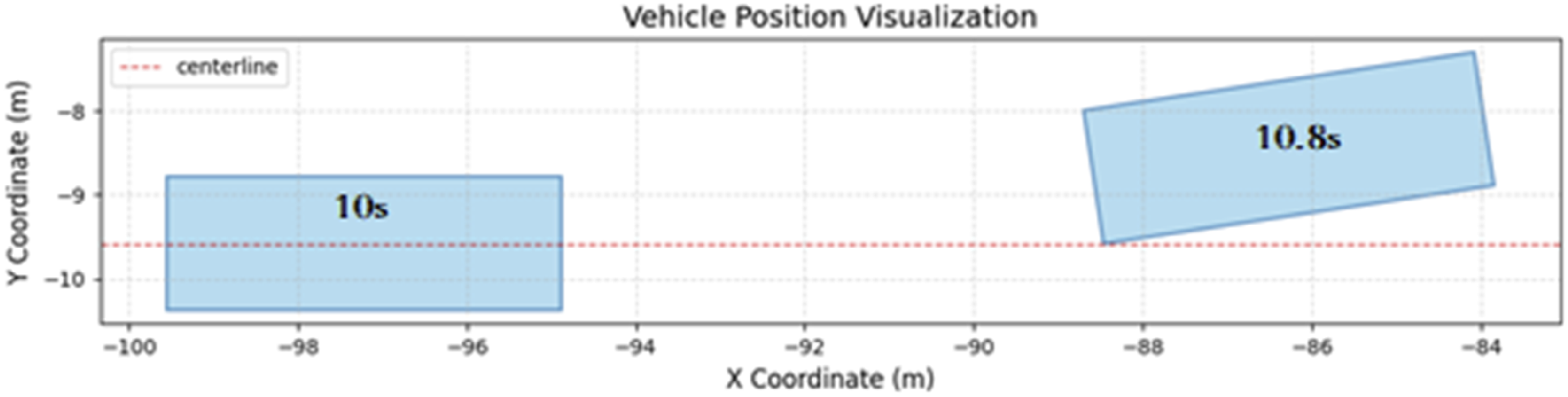

By analyzing the test data of this scenario, we simulated and determined the influence of the preceding vehicle’s lane change behavior on the starting time of the main vehicle’s deceleration, providing a reference basis for subsequent experiments and generalization tests. This allows us to simulate the adaptability of the main vehicle to changes in the preceding vehicle’s behavior and determine that the response time of the main vehicle will directly affect the evaluation of its risk avoidance capability.

Experimental results overview: Basic and controlled variable experiments

Through the test experiment, we have effectively set up the braking event of the main vehicle. That is, the host vehicle initiates the braking operation 0.8 s after the front vehicle changes lanes providing a reference for the scenario setup of the basic experiment.

In the basic experiment of section 3.3, the main vehicle successfully stops after decelerating, while the front vehicle (VT2) remains stationary. We recorded the stationary positions of the main vehicle and the front vehicle through the VTD platform. The specific data is shown in Table 4. The vehicle coordinates are the center point coordinates, with the X-coordinate representing the vehicle’s position in the driving direction and the Y-coordinate representing the vehicle’s lateral position.

Table 4.

Position coordinates of main vehicle and front vehicle.

Vehicle name	X-coordinate (m)	Y-coordinate (m)	Vehicle length (m)
Ego	−58.5176	−9.375	4.674
VT2	−50	−9.375	4.674

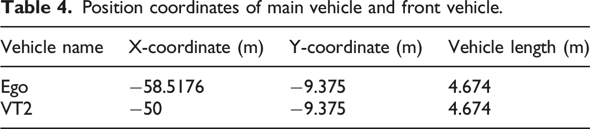
From the above table, it can be calculated that the stationary distance between the main vehicle and the front vehicle is:

Distance S = | X_{Ego} - X_{VT 2} | - \frac{L_{Sum of Vehicle Lengths}}{2} = 3.85 m

The experiment demonstrates that the main vehicle successfully braked and avoided a collision with the stationary front vehicle, indicating that this is a good set of following parameters that can effectively prevent sudden incidents.

In the controlled variable experiments of section 3.4, the coordinate information of the main vehicle and the front vehicle is shown in Table 5.

Table 5.

Generalization scenario position coordinates.

Scenario number	Vehicle name	X-coordinate (m)	Y-coordinate	Vehicle length (m)	Collision occurrence
Standard	VT2	−50	−9.375	4.674
1	Ego	−48.52	−9.375	4.674	Yes
2	Ego	−53.19	−9.375	4.674	Yes
3	Ego	−51.58	−9.375	4.674	Yes
4	Ego	−39.06	−9.375	4.674	Yes

In the above experiments, we conducted targeted research by adjusting and controlling parameters such as the following distance of the main vehicle, the lane change moment of the preceding vehicle, and the driving speed of the vehicles. The experiments show that in some scenarios, the main vehicle failed to brake in time, resulting in a collision with the front vehicle.

Experimental results overview: Generalization experiment

In the generalization experiment, the experimental results are shown in Figure 6. Regarding the final states of the two vehicles in the figure after the test, we use three colors for identification. The first is red, indicating a collision between the two vehicles, suggesting that this following state is unacceptable. The second is yellow, indicating that although no collision occurred between the two vehicles, the distance between the rear of the following vehicle and the front of the preceding vehicle along the road direction is less than 4 m when the vehicles are stationary. In other words, when the main vehicle travels at a speed of 60 km/h, the collision time between the two vehicles is TTCv = 60 < 0.25 s, indicating that although this state can avoid a collision, there is still a significant risk. The third is green, indicating that no collision occurred between the two vehicles, and the distance between them after stopping is greater than 4 m, suggesting that the vehicle operation is relatively safe.

Figure 6.

Experimental results display.

The overall experimental results present a pattern of green in the upper left and red in the lower right. The experiments indicate that when the speed is relatively fast or the following distance is relatively close, the main vehicle has a high risk of collision with the stationary front vehicle, and collisions may even occur. By maintaining a good distance from the preceding vehicle or maintaining a lower driving speed, the collision risk of the main vehicle can be significantly reduced.

Experimental results analysis

Through the above experimental overview, we have gained an intuitive impression of the experimental scenario of “front vehicle stationary, preceding vehicle suddenly cutting out, and main vehicle decelerating to avoid collision.”

Taking the basic experimental scenario as an example, the distance between the main vehicle and the preceding vehicle is 25 m. The preceding vehicle changes lanes when TTC_{VT1_VT2} is 1.5 s, and then the main vehicle recognizes the stationary vehicle ahead and starts braking after approximately 0.8 s. The maximum reaction distance provided to the main vehicle is:

S_{M a x i m u m R e a c t i o n D i s t a n c e} = L_{E g o_V T 1} + v ({T T C}_{V T 1_V T 2} - 0.8) - \frac{L_{Sum of Vehicle Lengths}}{2} = 32.00 m

Half of the vehicle length is subtracted because the vehicle coordinates recorded in the CSV are the coordinate positions of the vehicle center, and a collision event occurs when the rear of the vehicle is hit.

Therefore, the main vehicle needs to successfully brake within this distance to avoid a collision. In this scenario, the actual reaction distance of the vehicle is: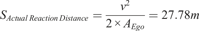

S_{A c t u a l R e a c t i o n D i s t a n c e} = \frac{v^{2}}{2 \times A_{E g o}} = 27.78 m

In the basic experiment, the main vehicle avoided a collision. The theoretical remaining distance was 32 m–27.78 m = 4.22 m, which is within the allowable error range of the actual remaining distance S = 3.85 m in section 4.2. In the controlled variable experiments of section 3.4, using the above calculation method, the maximum remaining distances and theoretical remaining distances in each scenario experiment are obtained as shown in Table 6.

Table 6.

Generalization scenario data analysis.

Scenario number	Maximum reaction distance (m)	Actual reaction distance (m)	Theoretical remaining distance (m)	Actual remaining distance (m)
1	22	27.78	−5.78	−6.15
2	28.56	27.78	0.78	−1.48
3	32	34.72	−2.72	−3.09
4	35.89	49.38	−13.49	−15.61

Furthermore, we found that the actual remaining distance is always smaller than the theoretical remaining distance. This is because when we calculate, the deceleration A_Ego is directly taken as the maximum value of 5, but when braking a vehicle in the simulation software or the real world, the vehicle’s deceleration gradually increases to the maximum value, taking a period of time to change. This leads to a larger average deceleration value in the theoretical calculation, resulting in the theoretical remaining distance being greater than the actual remaining distance, as shown in the above table.

In the generalization experiment, we studied the relationship between the inter-vehicle distance and the vehicle speed while controlling the deceleration A_Ego and the reaction time TTC. Theoretically, if we want the vehicle to avoid a collision, the relationship between the two is: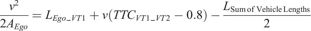

\frac{v^{2}}{2 A_{E g o}} = L_{E g o_V T 1} + v ({T T C}_{V T 1_V T 2} - 0.8) - \frac{L_{Sum of Vehicle Lengths}}{2}

Substituting the previous formula and specific values: A_Ego = 5 m/s², L_{Sum of Vehicle Lengths} = 4.674 m, TTC_{VT1_VT2} = 1.5 s, we can obtain the simplified formula:

L_{E g o_V T 1} = \frac{v^{2}}{10} - \frac{7 v}{10} + 2.337

Drawing this curve in Figure 7.

Figure 7.

“Distance-speed” curve.

In our generalization experiment, the value ranges of the following distance and vehicle speed are [15, 35] and [50, 80], respectively. This is consistent with our experimental results in the monotonically increasing part of this parabolic curve. Moreover, this curve is located at the boundary between the yellow and red squares, effectively describing the relationship between the following speed and following distance that vehicles should adhere to.

Furthermore, we can observe that when the vehicle speed is low, the change in the following distance is relatively gradual. However, when the vehicle speed is high, the required following distance increases significantly. In particular, when the vehicle speed exceeds a certain threshold, the growth of the following distance increases exponentially. This indicates that as the vehicle’s driving speed increases, the driver or the autonomous driving system needs to reserve a longer safety distance for potential collision risks.

Additionally, similar to the controlled variable experiments, there is an error in the vehicle deceleration A_Ego in the generalization experiment. In fact, L-v parabolic curve should move toward the upper left and narrow its opening, so that the red points originally on the “distance-speed” curve will then be below the curve.

Conclusions

This study constructed an experimental scenario of “front vehicle stationary, preceding vehicle suddenly cutting out, main vehicle decelerating to avoid collision” through a simulation platform and verified the safety and stability of the autonomous driving system through basic experiments and generalization experiments. The main conclusions are as follows:

(1) In general scenarios such as the basic experiment, when the recognition and response are timely, the vehicle can avoid collisions relatively smoothly, verifying the effectiveness of the experimental scenario and model.

(2) The controlled variable experiment shows the state of host vehicle following another vehicle, and factors including environmental conditions all have significant impacts on the collision outcome. For example, on the wet and slippery road, an additional distance is required to keep away from the front vehicle. In extreme cases, the system fails to avoid a collision, revealing its performance boundaries.

(3) The generalization experimental results clarify the relationship between the safe following distance and vehicle speed. In practical applications, especially in the design and testing process of autonomous vehicles, the influence of vehicle speed on the safe following distance must be fully considered. A dynamic adjustment strategy for the following distance should be adopted to ensure that a sufficient safety distance can be maintained even at high speeds, effectively preventing potential collision risks.

Footnotes

ORCID iDs

Ke Zhang

Yang Zhang

Funding

The authors disclosed receipt of the following financial support for the research, authorship, and/or publication of this article: Supported by the Science and Technology Research Program of Chongqing Municipal Education Commission (Grant No. KJQN202303223); and the Doctoral Fund Project of Chongqing Industrial Vocational and Technical College (2022GZYBSZK1-01).

Declaration of conflicting interests

The authors declared no potential conflicts of interest with respect to the research, authorship, and/or publication of this article.

References

Zhu

Zhang

Liu

. A safety evaluation method for autonomous vehicles based on natural driving data. China J Highw Transp 2022; 35(7): 283–291.

Liao

Chu

Cheng

. Review of the construction method of the scenario library system for autonomous driving simulation testing. Mach Manuf Aut 2024; 53(4): 271–275.

Wang

. Review of scenario generation methods for autonomous vehicle simulation testing. Autom Eng 2024; 7: 1–10.

Wang

. Design of obstacle avoidance system for electrically-powered autonomous vehicles. Autom Test Report 2023; 14: 10–12.

Sun

Zhang

Zhao

, et al. Strategy modeling and simulation of interactive scenarios for autonomous driving testing. Automot Eng 2024; 46(11): 1962–1972.

Luo

Zheng

. Research on autonomous driving simulation testing based on digital twin. Modern Comp 2023; 29(9): 1–8.

China Automotive Engineering Research Institute Co., Ltd . Intelligent driving index leads intelligent driving (highway). Chongqing: China Automotive Engineering Research Institute Co., Ltd, 2023.

Huang

Liu

, et al. Intelligence testing for autonomous vehicles: a new approach. IEEE Trans Intell Veh 2017; 1(2): 158–166.

Liu

Zhao

Qin

. Behavior decision-making of vehicle assisted driving based on dynamic risk assessment. Automot Eng 2024; 46(11): 2005–2016.

10.

Liu

Zhang

. Research progress of virtual simulation testing technology for autonomous driving. China Sci Paper 2021; 16(6): 571–577+584.

11.

Jiang

Dang

, et al. A review of the research progress on scenario testing of autonomous vehicles. Autom Tech 2022; 8: 10–22.

12.

Wang

Zhang

Zhou

, et al. A method for replicating intelligent driving simulation scenarios based on VTD. Autom Sci Tech 2022; 3: 56–60.

13.

Abdelhamid

Bennoud

Zeroual

. Uncertainty quantification and sensitivity analysis of concrete structure using multi-linear regression technique. Science. 2025; 5(1): 240–258.

14.

Zhang

Jiao

Sang

, et al. Simulation of Latin hypercube sampling for parameters of vehicle body response surface model. Comput Simulat 2021; 38(7): 123–127.

15.

Zhu

Tang

Zhao

, et al. An accelerated testing method for intelligent driving systems based on surrogate genetic optimization. J Tongji Univ Nat Sci 2024; 52(4): 501–511.