English text sentiment analysis model using LSTM algorithm

Abstract

Traditional English text sentiment analysis models have limitations in handling complex texts and long-term dependency relationships, leading to an impact on the accuracy and deep understanding of sentiment analysis. This article aims to solve the above problems by applying the LSTM (long short-term memory) algorithm. First, the data is cleaned and preprocessed, including regular expressions, word segmentation, stop word filtering, and stem extraction. Next, a sentiment lexicon is utilized to annotat. Word2Vec and TF-IDF are combined for feature vectorization, and the positional encoding is applied. An LSTM network structure is then constructed. After training optimization, the model achieves an accuracy of up to 90% on the test set, outperforming other models. The LSTM algorithm effectively solves the limitations of traditional models and achieves higher accuracy. In summary, the application of LSTM algorithm in English text sentiment analysis models can effectively address existing limitations and make them more accurate.

Keywords

sentiment analysis model long short-term memory English text data preprocessing model training and optimization

Introduction

With the explosive growth of social media and online content, a large amount of textual data needs to be analyzed and understood. Sentiment analysis can help businesses and organizations understand the public’s sentiment tendencies and make more informed decisions. Automated sentiment analysis of English texts becomes particularly critical. However, although traditional English text sentiment analysis models perform well on simple texts, their ability to handle English texts with complex structures and long-term dependencies is often limited. These limitations not only affect the accuracy of sentiment analysis, but also hinder the model’s understanding of the deep meaning of the text. Therefore, this article applies an English text sentiment analysis model based on LSTM algorithm to improve the accuracy and depth of sentiment analysis.

LSTM can handle long-term dependencies and improve the efficiency of feature extraction, thereby optimizing the processing of contextual information. In addition, training can be done on diverse datasets. In terms of research structure arrangement, this article first introduces the preprocessing process of data, then describes in detail the steps of using Word2Vec and TF-IDF methods for feature vectorization, and introduces positional encoding to enhance the model’s ability to capture contextual information. On this basis, this article constructs a network structure based on LSTM for sentiment analysis, and ensures that the model achieves optimal performance through multiple training and parameter optimization. Finally, the accuracy and generalization ability of the model can be evaluated by validation on different test sets.

Compared with the existing researches, this article innovatively combines LSTM network with Word2Vec, TF-IDF and positional encoding to construct an efficient English text sentiment analysis model, which provides a new research perspective and method for the field of sentiment analysis. The main contribution of this article is the construction of an LSTM network structure applied to English text sentiment analysis models. Experimental results have shown that this model performs better on the test set than various existing sentiment analysis models, significantly improving the accuracy and depth of sentiment analysis. In addition, this article also explores the application of positional encoding in sentiment analysis, providing a new perspective and methodological foundation for subsequent research. The research structure of this article is shown in Figure 1.

Figure 1.

Research structure of this article.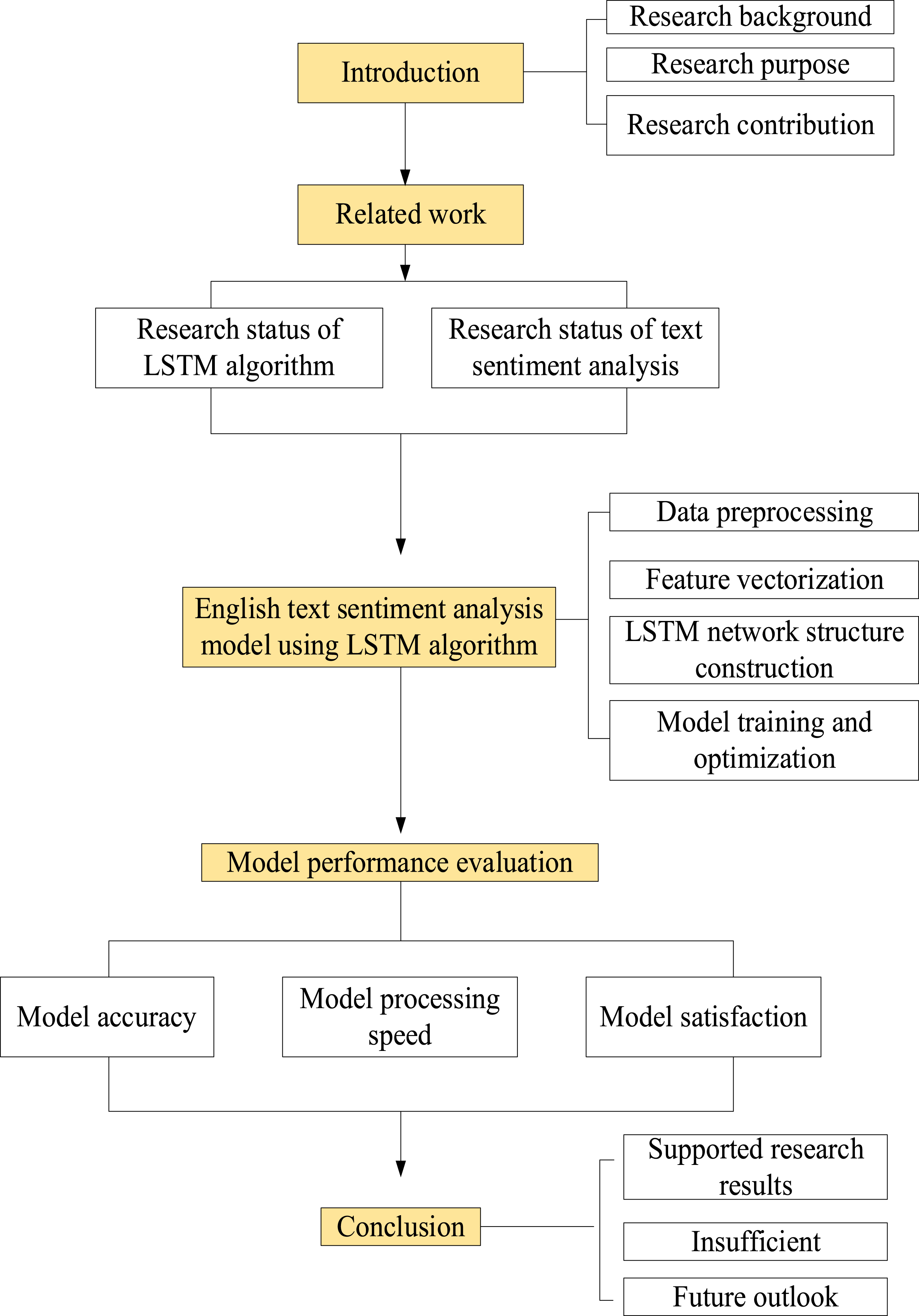

Related work

The amount of text data is huge, and sentiment analysis helps to understand public emotions, which is of great significance for decision-making in many fields.^1,2 Currently, many scholars are actively exploring advanced technologies for sentiment analysis.^3,4 Raza⁵ used machine learning techniques for sentiment analysis of scientific texts, mainly using three steps: data preprocessing, feature extraction, and model training to complete sentiment classification. However, there are shortcomings in the experimental evaluation of this study, as detailed performance indicators and comparative results were not provided. Yadav⁶ reviewed methods for sentiment analysis using deep learning architectures, studied various deep learning models, and described their structures and working principles. However, the study also did not provide detailed experimental settings and evaluation of performance. The application of Bonta⁷ in sentiment analysis uses dictionary-based methods. He investigated different dictionaries and emotional vocabulary resources and compared the performance of relevant methods. However, his research lacks an analysis of the advantages and disadvantages of relevant methods. D’Aniello⁸ proposed a reference model called KnowMIS-ABSA for applying sentiment analysis. This model is built based on preprocessing, feature extraction, and classifier training. However, he did not provide detailed model implementation and performance evaluation results. Hartmann⁹ evaluated the accuracy of different sentiment analysis methods and discussed the application of sentiment analysis in the field of marketing. He proposed a new sentiment analysis method and analyzed its effectiveness in consumer behavior prediction and market trend analysis. However, he did not provide specific method details and experimental results. The above literature elaborates on some research work in the field of sentiment analysis, covering different methods and techniques. However, these studies all have some shortcomings, so this article studies an English text sentiment analysis model using LSTM algorithm.

The LSTM algorithm is particularly adept at handling and predicting long-term dependency problems in time series data.^10,11 LSTM can also address the drawbacks of traditional neural networks by introducing gating mechanisms to enable models to learn when to forget old information and when to introduce new information.^12,13 Park¹⁴ studied using the LSTM algorithm to predict high turbidity in rivers. By constructing a model that can understand the characteristics of time series data, the accuracy of predicting sudden changes in river turbidity can be improved. This is significantly helpful for preventing environmental disasters and developing emergency measures. Accurately predicting the development of the epidemic on a global scale is crucial for the effective implementation of public health interventions and resource allocation. Kim¹⁵ used LSTM algorithm to analyze and learn time series data of the epidemic and predict the spread trend of COVID-19. Zhang¹⁶ studied the use of LSTM algorithm as a sequence to sequence data modeling method for monthly peak load forecasting in the power system 3 years ago. This method combines the spatial feature extraction ability of CNN and the time series analysis ability of LSTM, which greatly improves the accuracy of prediction. Antenna wetting has a significant impact on the transmission characteristics of microwave links, and Pu¹⁷ proposes an E-band microwave link wet antenna attenuation model based on LSTM algorithm. The use of LSTM algorithm to model and predict the attenuation effect of wet antennas under complex weather conditions has a positive impact on improving the reliability of microwave communication. ShanYou¹⁸ successfully developed a single instrument seismic intensity prediction model based on long short-term memory neural networks. This model can utilize the time series characteristics of short-term seismic parameters to efficiently and accurately predict the maximum seismic intensity, with good timeliness and low rates of missed and false alarms. In summary, the LSTM algorithm, as a powerful time series data analysis tool, has demonstrated its unique advantages in prediction tasks in multiple fields. These demonstrate its suitability for constructing sentiment analysis models for English texts.

Method

Data preprocessing

This article collects English text data from different channels and preprocesses it, as shown in Figure 2.

Figure 2.

Data preprocessing operation diagram.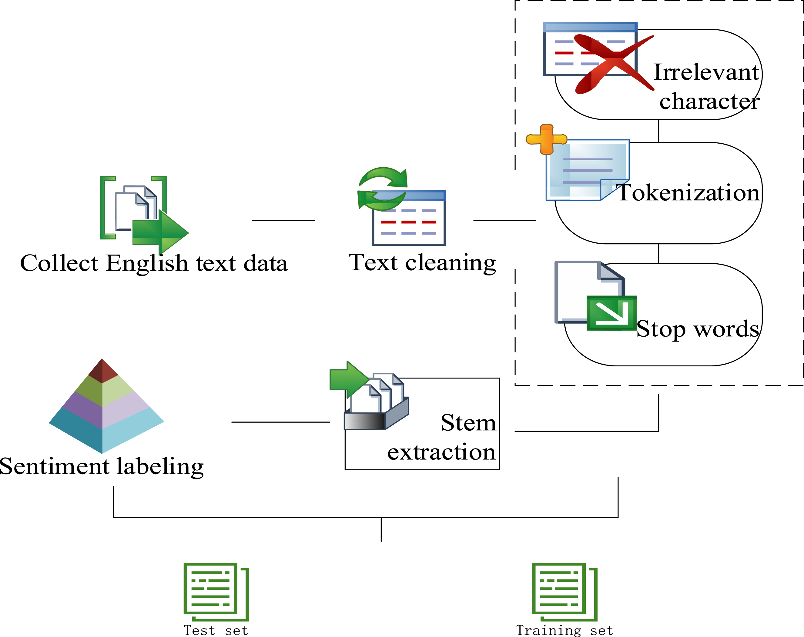

Figure 2 shows the text cleaning operation performed after data collection is completed, using the regular expression library in programming languages to efficiently remove irrelevant characters. The specific operations are: removing the label first, then punctuation, followed by numbers and lowercase. Then, the text can be segmented by using the word_tokenize function in the natural language processing library to decompose the text string into individual vocabulary units. In order to reduce the amount of words that the model needs to process, the list of stop words provided by the natural language processing library is used to filter and remove stop words (referring to words that frequently appear in the text but do not contribute significantly to sentiment analysis, such as articles: a, an, and the; pronouns: I, you, he, she, it, we, and they; auxiliary verbs: is, are, was, were, be, been, and being; prepositions: in, on, at, by, for, with, and about; conjunctions: and, or, but, if, and because; other common words: this, that, there, here, and some).

After filtering, the Porter stem extraction algorithm can be used to perform stem extraction processing, restoring words to their root form so that different forms of words can be recognized by the model as the same input.¹⁹ Through stem extraction, words like “running,” “ran,” and “runs” are simplified to the basic form “run.”

After completing the promotion process, it can be determined whether the emotional tendencies expressed in each paragraph of the text are positive, negative, or neutral, that is, by using a pre-defined sentiment dictionary (which contains a large number of words with sentiment polarity labels) to annotate the sentiment polarity of the text, the model can learn the emotional colors carried by different words.

The train_test_split function in the Scikit-learn library can be used to partition the preprocessed dataset into training and testing sets, ensuring that the dataset is randomly partitioned and has diversity and generalization. A ratio of 80% training and 20% testing for the training and testing sets is specified. The fixed random seed is 42 to ensure the reproducibility of the results.

Feature vectorization

Feature vectorization is a crucial step in sentiment analysis, which transforms natural language texts into numerical features that machine learning algorithms can process. This article adopts a two-stage approach for feature vectorization: first, pre-trained word embeddings are used, and then positional encoding is introduced to enhance the representation of contextual relationships. In text intensive data, pre-trained word embeddings can effectively capture the semantic information of vocabulary and improve the quality of feature vectors. In real-time monitoring environments, positional encoding can enhance the model’s ability to process time series data and improve prediction accuracy.

On the basis of large-scale corpus training, a pre-trained Word2Vec model is obtained to collect rich semantic information. Each word in the text can be mapped into a fixed size vector to capture the semantic relationship between words.^20,21 In this way, the model can infer the semantic similarity between words based on the distance in the vector space while recognizing the meaning of words.

To maintain consistent text sequence length, padding operations can be performed. The maximum length of the sequence is T. For sequences with a length less than T, zero vectors are used for padding:

{x_{i}}^{‘} = {\begin{cases} \begin{array}{l} x_{i} & i f i < n \end{array} \\ \begin{array}{l} 0 & i f i > n \end{array} \end{cases}

(1)

x_{i}

refers to the

i

th word.

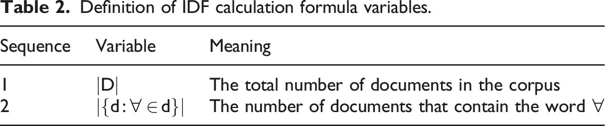
In order to further improve the expression ability of features, this article introduces a weighting mechanism based on TF-IDF, considering the frequency of words appearing in the entire dataset, and assigning lower weights to common but indistinguishable words. Assigning higher weights to keywords with high discrimination can reduce the interference of common words on the model’s judgment of emotions and improve the model’s sensitivity to key emotional words.^22,23

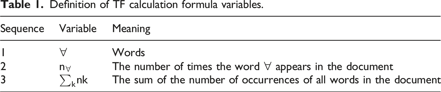
The calculation of TF in TF-IDF is:

TF (\forall) = \frac{n_{\forall}}{\sum_{k} nk}

(2)

The definition of variables in the calculation formula for TF is shown in Table 1.

The calculation of IDF in TF-IDF is:

IDF (\forall) = \log \frac{| D |}{| {d : \forall \in d} |}

(3)

Table 1.

Definition of TF calculation formula variables.

Sequence	Variable	Meaning
1	$\forall$	Words
2	$n_{\forall}$	The number of times the word $\forall$ appears in the document
3	$\sum_{k} nk$	The sum of the number of occurrences of all words in the document

The definition of IDF calculation formula variables is shown in Table 2.

Table 2.

Definition of IDF calculation formula variables.

Sequence	Variable	Meaning
1	$\| D \|$	The total number of documents in the corpus
2	$\| {d : \forall \in d} \|$	The number of documents that contain the word $\forall$

On the basis of word embedding and TF-IDF weighting, attention can be paid to the positional information of words in sentences. By designing a positional encoding strategy, each word can be assigned a positional vector, which enables the model to better capture long-distance dependencies, namely, the relationship between preceding and following words in the text. Positional encoding assigns each word an information vector reflecting its position in the sentence, which enhances the model’s ability to understand the text order. Among them, positional encoding generated by sine and cosine is popular for its ability to capture periodic patterns and is often used in combination with word embedding in pre-trained models to improve the model’s performance on sequence data processing tasks such as sentiment analysis. Comparing different strategies, it is found that sine and cosine encoding is often better than simple position index coding, which can capture long-distance dependencies more effectively, thus improving the overall effect of the model. The positional encoding is added directly to the word vector generated by Word2Vec to form the final word representation. When positional encoding is combined with TF-IDF, TF-IDF is used as the weight and multiplied with the word vector.

Three words can be used to demonstrate the specific operation of feature vectorization, as shown in Table 3.

Table 3.

Specific operations of feature vectorization.

Word	Word2Vec vector	TF-IDF weight
Happy	[0.25, −0.12, 0.34, ...]	0.098
Sad	[−0.32, 0.15, −0.21, ...]	0.075
Joy	[0.41, −0.08, 0.29, ...]	0.102

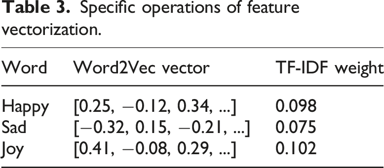
Table 3 lists three emotional words “happy,” “sad,” and “joy,” each of which was transformed into corresponding word vectors through a pre-trained Word2Vec model. This vectorization processing helps the model capture the semantic features of vocabulary. Meanwhile, Table 3 also provides the TF-IDF weights for each word. This weight combines word frequency and inverse document frequency to emphasize the importance of important vocabulary and weaken the interference of common vocabulary. The TF-IDF weight of “Happy” is 0.098, while “joy” is 0.102, indicating that “joy” is slightly more important in distinguishing emotions in documents than “Happy.”

LSTM network architecture construction

LSTM effectively solves the long-term dependency problem through its gating mechanism and cell state design, providing a more stable gradient flow than traditional RNN, thus enabling the learning of complex dependency relationships across multiple time steps. Compared to Transformers, LSTM may have advantages in handling specific types of long-term dependencies, but Transformers are typically superior in computational efficiency and performance for certain tasks. Both have their own strengths in the field of sequence processing.

A recursive neural network based on LSTM units can be designed within the English text sentiment analysis model to handle and predict long-term dependency problems in sequence data. The specific architecture is shown in Figure 3. In Figure 3, the parameters of the LSTM network include the size of the input layer, hidden layer, and output layer. The first step is to initialize them.^24,25 Next, this article selects a multi-layer structure containing multiple LSTM layers to capture complex structures and deep semantic information in text data. The LSTM model encounters challenges such as high computational resource requirements, sequence length limitations, and contextual information attenuation when processing long texts. The complexity of specific emotional expressions in sentiment analysis, including emotional mixing, emotional inflection, implicit emotional expression, emotional intensity, and context dependence, further increases the difficulty of sentiment analysis tasks. Each LSTM layer is composed of multiple LSTM units, each containing a forget gate, input gate, and output gate, which control the transmission and memory of information flow.

Figure 3.

LSTM network structure.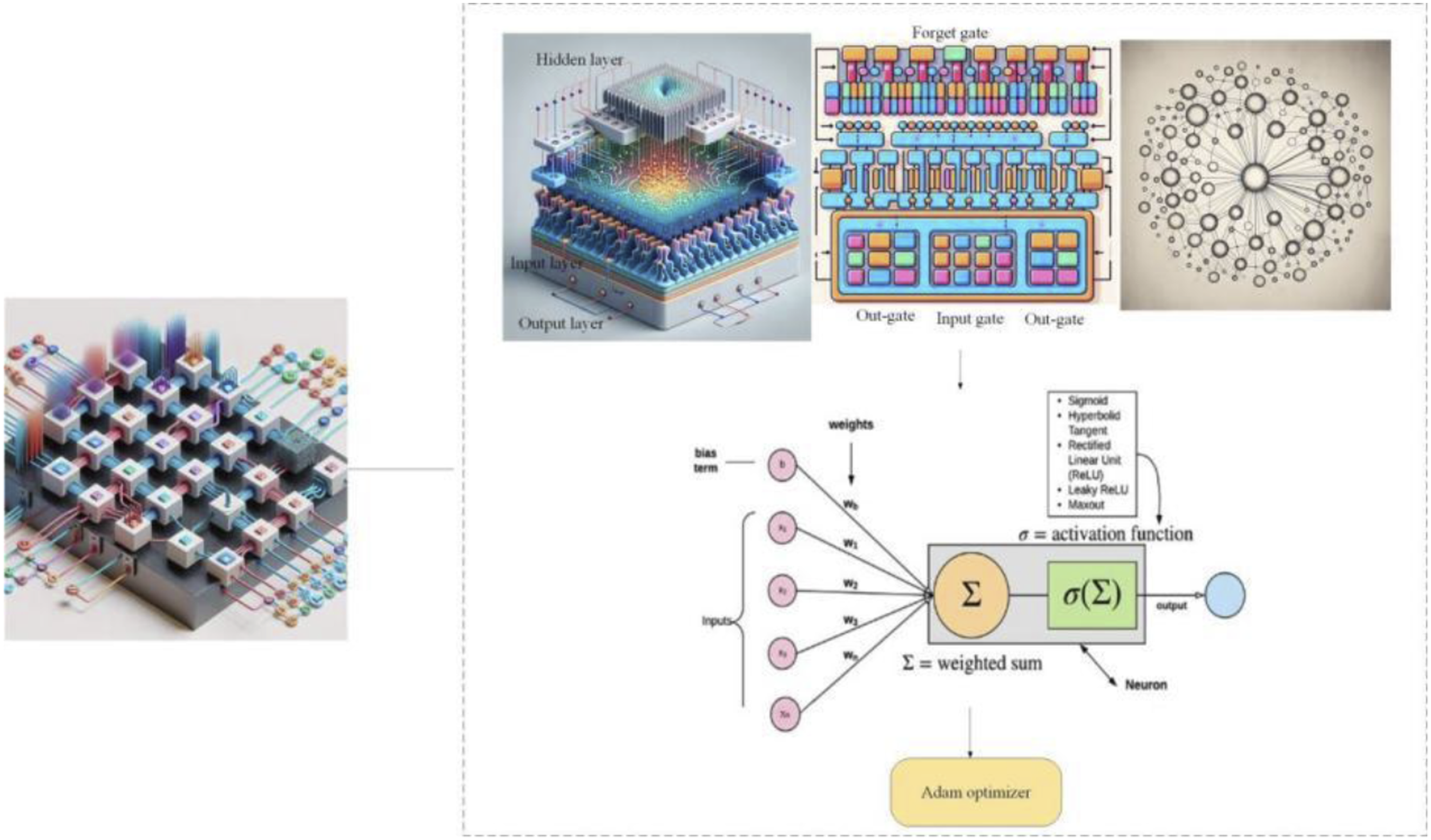

The gating states of forget gate ( $f_{t}$ ), input gate ( $i_{t}$ ), and output gate ( $o_{t}$ ) are calculated as follows:

{\begin{cases} f_{t} = σ (W_{x_{f}} x_{t} + W_{h_{f}} h_{t - 1} + W_{c_{f}} c_{t - 1} + b_{f} \\ i_{t} = σ (W_{x_{i}} x_{t} + W_{h_{i}} h_{t - 1} + W_{c_{i}} c_{t - 1} + b_{i} \\ o_{t} = σ (W_{x_{o}} x_{t} + W_{h_{o}} h_{t - 1} + W_{c_{o}} c_{t - 1} + b_{o} \end{cases}

(4)

The variable definition of the gate control state calculation formula is shown in Table 4.

Table 4.

Definition of calculation formula variables for gate control states.

Sequence	Variable	Meaning
1	$t$	Time step
2	$W$	Weight
3	$b$	Bias parameters
4	$σ$	Sigmoid function
5	$h_{t}$	The hidden state of the current moment
6	$c_{t}$	The state of the unit at the current moment
7	$h_{t - 1}$	The hidden state of the previous moment

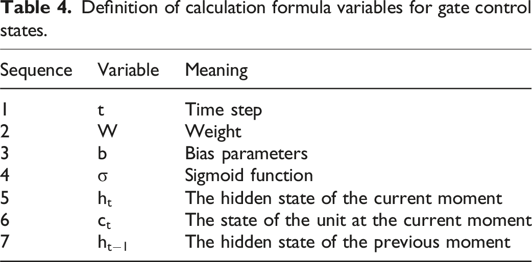
For each time step $t$ , the LSTM unit receives the hidden state and input from the previous time step, and outputs the hidden state and unit state at the current time step. $W$ refers to the weight, $b$ refers to the bias parameter, $σ$ refers to the sigmoid function, $h_{t}$ and $c_{t}$ refer to the hidden state and unit state at the current time. $h_{t - 1}$ refers to the hidden state of the previous moment.

The $h_{t}$ sum of $c_{t}$ in the calculation is as follows:

{\begin{cases} {\bar{c}}_{t} = \tanh (W_{x_{c}} x_{t} + W_{h_{c}} h_{t - 1} + b_{c}) \\ c_{t} = f_{t} ⨀ c_{t - 1} + i_{t} ⨀ {\bar{c}}_{t} \\ h_{t} = o_{t} ⨀ \tanh (c_{t}) \end{cases}

(5)

{\bar{c}}_{t}

represents the candidate unit status at the current time, while

⨀

refers to element wise multiplication.

In the LSTM network, the input for each time step is a high-dimensional feature vector generated during the feature vectorization process, which contains the word embedding and position encoding information obtained in the preprocessing step. Each unit in the LSTM layer can calculate a new hidden state and unit state based on the current input and previous hidden state. This allows the network to remember and utilize the information from previous steps, effectively handling long-distance dependencies.²⁶

To avoid overfitting, this article introduces Dropout layers between LSTM layers. The Dropout layer randomly discards some connections of neurons during the training process, reducing the model’s over sensitivity to training data and increasing the model’s generalization ability.^27,28 Then, from the output of the last LSTM layer, multiple fully connected layers (also known as dense layers) can be connected to map the high-dimensional output of the LSTM layer to the final emotional classification result. The activation function of the fully connected layer uses ReLU (Rectified Linear Unit)^29,30 and the softmax activation function to allow the output layer to convert the output of the fully connected layer into a probability distribution. These probabilities directly correspond to each emotional category.

In the process of designing LSTM networks, the optimal number of hidden layer units and learning rate can be selected through cross validation. To determine the optimal number of hidden layer units, a parameter range between 10 and 1000 is first tried. Next, a 5-fold cross validation is used to evaluate the performance of models with different numbers of hidden layer units. Finally, the optimal number of hidden layer units is determined to be 350, with a learning rate of 0.01. The optimal parameter combination for Adam optimizer is β1 = 0.9 and β2 = 0.999. Meanwhile, the Adam optimizer was used to adjust the network weights and accelerate the gradient descent process through momentum, reducing oscillations and making the training more stable. As it combines the advantages of momentum and adaptive learning rate, effectively accelerating network training and improving model performance.

Model training and optimization

Random gradient descent is used as the basic optimization algorithm for model optimization, and an early stopping mechanism is introduced during the training process to monitor performance indicators on the validation set. Once it is found that the performance of the model no longer improves after multiple consecutive epochs, the training process can automatically stop. This can avoid overfitting of the model on training data, while retaining the model’s generalization ability on unseen data.

In addition to random gradient descent, L2 regularization technique is also used, which adds a weight decay term to the loss function to limit the size of model parameters and reduce the complexity of the model. The selection of regularization parameters can be determined through grid search and cross validation, ensuring that the model maintains high prediction accuracy while minimizing the risk of overfitting.

During the model training process, a learning rate decay strategy can be implemented. As training progresses, the learning rate can be gradually reduced, which helps the model adjust parameters more finely in the later stages of training, avoiding excessive jumps in the parameter space, and thus improving the stability and final performance of the model. To further optimize model performance, batch normalization technology can be introduced. Each batch of data can be standardized to reduce internal covariate bias. This can make model training more stable, while allowing for higher learning rates and accelerating training speed. The batch size in the training process is 64; the number of iterations is 30; the learning rate is 0.001.

After the model training is completed, hyperparameter tuning is performed, and grid search and cross validation are used to find the optimal hyperparameter group, so that the model achieves the best performance on the test set.

Model performance evaluation

Model accuracy

The existing English text sentiment analysis models include rule-based sentiment analysis model (M1), pre-trained language model (M2), aspect-based sentiment analysis model (M3), and multimodal analysis model (M4). The publicly available English text sentiment analysis dataset Twitter sentiment analysis dataset (the Twitter sentiment analysis dataset is a widely used dataset primarily used for sentiment analysis tasks, and this dataset contains a large number of tweets labeled with corresponding emotional tags such as positive, negative, and neutral) can be used. The dataset consists of 10,000 text samples, with positive and negative emotions accounting for half each. The dataset can be divided, with 80% used as the training set and 20% used as the testing set. The training set contains 8000 samples, and the test set contains 2000 samples. The accuracy of the model can be evaluated on the test set, which is the proportion of samples correctly predicted by the model on the test set. The confusion matrix of the computable model includes the number of true positives (TP), false positives (FP), true negatives (TN), and false negatives (FN). For data preprocessing on the training set, rule-based sentiment analysis model (M1), pre-trained language model (M2), aspect-based sentiment analysis model (M3), multimodal analysis model (M4), and English text analysis model (M5) using LSTM algorithm can be trained using the training set. During the training process, the performance of the model on the validation set can be monitored to avoid overfitting. The trained model can be evaluated using the test set, and the calculation accuracy can be recorded as the evaluation indicator. The results are shown in Table 5.

Table 5.

Predicted quantities of each model.

Model	Accuracy (%)	TP	FP	TN	FN
M1	80	1580	420	1610	390
M2	85	1700	300	1680	320
M3	83	1660	340	1650	350
M4	87	1740	260	1720	280
M5	90	1820	180	1780	220

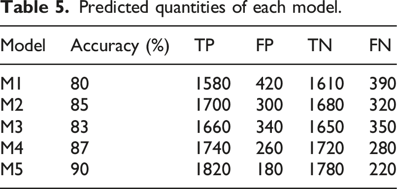
TP and TN in Table 5 represent the number of positive and negative emotion samples correctly predicted by the model. FP and FN are the number of positive and negative emotion samples that the model incorrectly predicted. It can see that the M5 model has the highest number of true and true negative cases among all models, with 1820 and 1780, respectively. This indicates that it performs well in predicting both positive and negative emotions. Meanwhile, the M5 model has the least number of false positive and false negative cases, with 180 and 220, respectively, which further demonstrates its excellent predictive ability.

The accuracy of the model can be calculated based on the data in Table 5,³¹ as shown in Figure 4. The accuracy formula is:

Accuracy = \frac{TP + TN}{TP + FP + TN + FN}

(6)

Figure 4.

Prediction accuracy of each model.

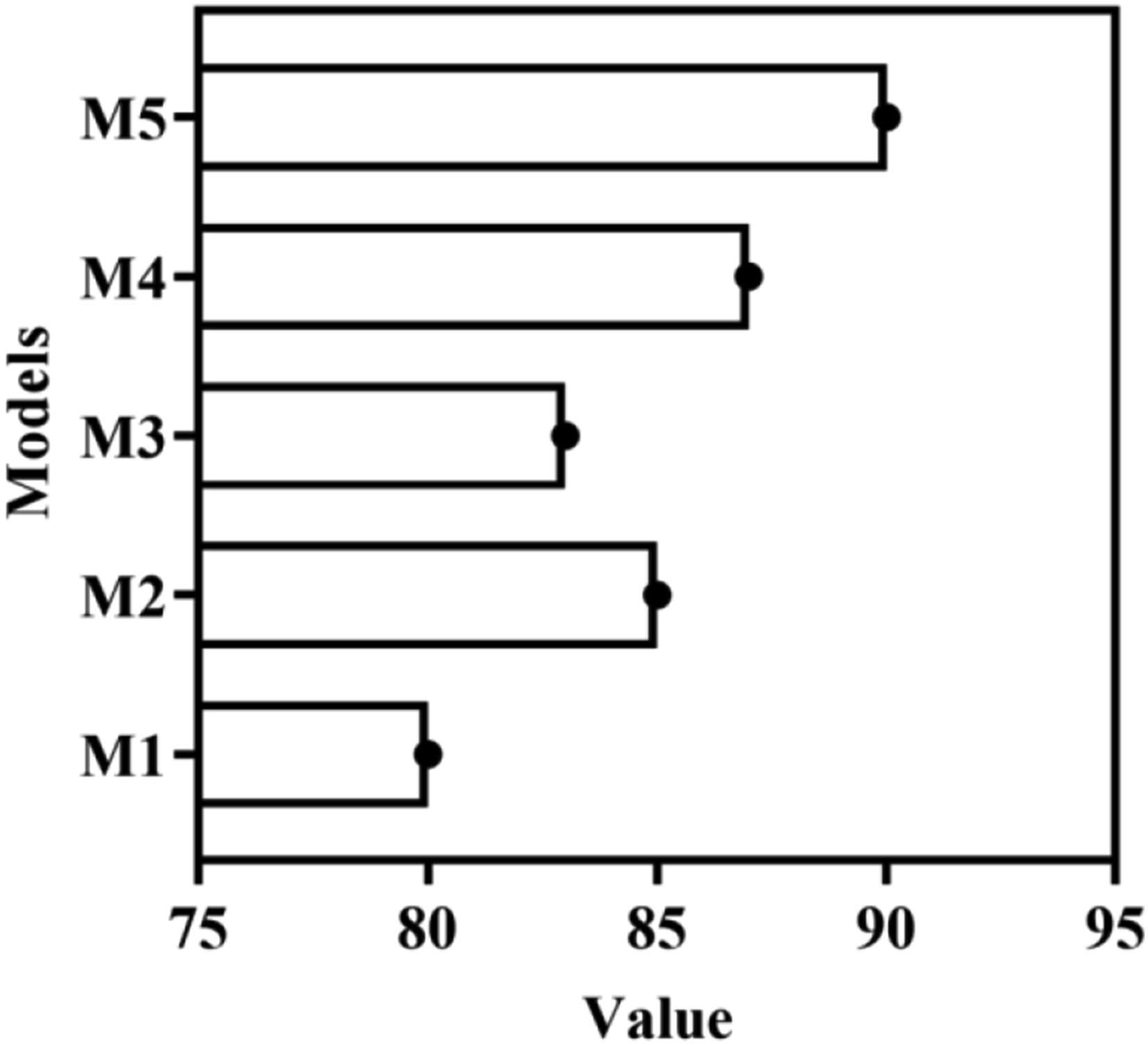
From the accuracy shown in Figure 4, M5 performs the best, with an accuracy of up to 90%, far exceeding other models and 3% points higher than the second ranked M4 model (with an accuracy of 87%). This indicates that the model using LSTM algorithm has excellent performance in handling English text sentiment analysis tasks.

The M5 model performs the best in predicting positive emotions, due to the context capture ability of LSTM, which can recognize texts containing multiple positive emotion expressions. The M5 model also performs well in predicting negative emotions, indicating that LSTM can effectively identify the expression patterns of negative emotions. Although Table 5 does not specifically list neutral emotions, it can be inferred that the M2 and M4 models may perform better in predicting neutral emotions, as pre-trained language models and multimodal models can capture more detailed information and help distinguish neutral emotions. Due to the use of a large amount of pre-training data and multimodal information, M2 and M4 are able to capture a wider range of emotional expressions, thereby improving prediction accuracy. M1 relies on manually formulated rules, making it difficult to handle complex and varied emotional expressions, resulting in relatively low accuracy. M1 can combine other algorithms to develop new rules to improve prediction.

In summary, the English text analysis model (M5) of the LSTM algorithm performs better than other types of models on the Twitter sentiment analysis dataset, both in terms of accuracy and the number of incorrectly predicted samples.

Model processing speed

To verify the processing speed of the model, the above 5 models were run in the same hardware and software environment to ensure the fairness of the experimental results. The specific configuration is to use a single NVIDIA Tesla V100 GPU (Graphics Processing Unit), the CPU (Central Processing Unit) is Intel Xeon E5-2680 v4@2.40GHz, and the memory is 64 GB. The time spent by each model in the three stages of data set preprocessing, feature vectorization, and emotion classification can be recorded, as shown in Figure 5. For the convenience of experiments, C1 can be used instead of data set preprocessing, C2 instead of feature vectorization, and C3 represents emotion classification.

Figure 5.

Processing time of the model.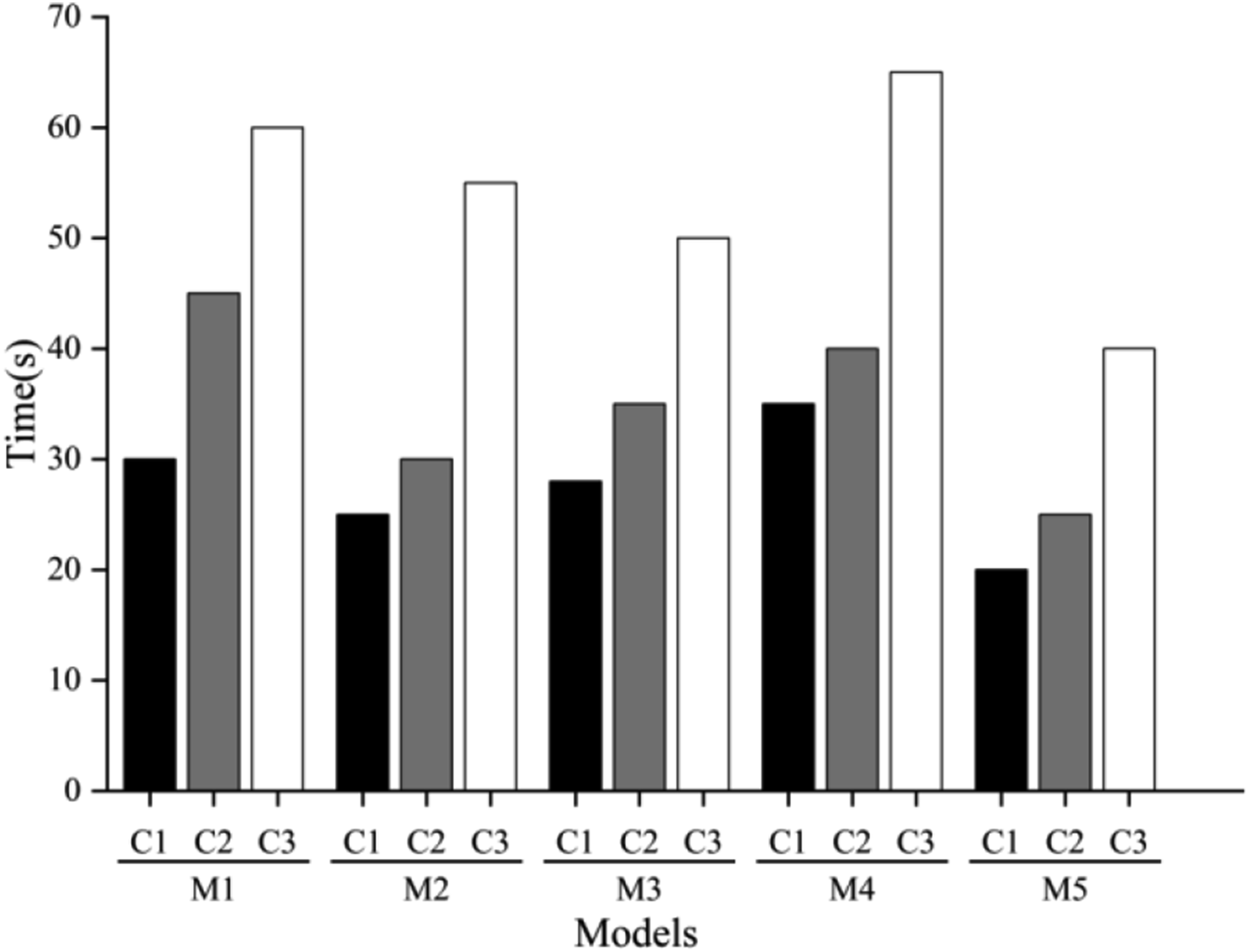

Figure 5 compares the processing time of five different models in the three stages of dataset preprocessing, feature vectorization, and sentiment classification. It is evident that all models take the longest time in the emotion classification stage.

Among them, M1 takes 30 s in the dataset preprocessing stage, 45 s in the feature vectorization stage, and 60 s in the sentiment classification stage. In contrast, M2 has a faster processing speed, taking only 25 s, 30 s, and 55 s, respectively. The processing time of M3 is 28 s, 35 s, and 50 s in three stages, while M4 requires 35 seconds, 40 s, and 65 s. Finally, M5 performs the best among all models, requiring only 20 s for dataset preprocessing, 25 s for feature vectorization, and 40 s for sentiment classification. By comparing these data, it was found that M5 has significantly better processing speed than other models, indicating its high efficiency in English text analysis.

The total processing time of each model can be calculated based on the data in Figure 5, as shown in Table 6.

Table 6.

Total processing time of each model.

Model	Total processing time (s)	Total processing time (min)	Total processing time (h)
M1	135	2.25	0.0375
M2	110	1.83	0.0305
M3	113	1.88	0.0313
M4	140	2.33	0.0388
M5	85	1.42	0.0237

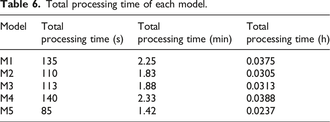
Table 6 shows that the total processing time of M1 is 135 seconds, which is equivalent to 2.25 min or 0.0375 h. The processing speed of M2 is slightly faster, with a total processing time of 110 s, which is 1.83 min or 0.0305 h. The total processing time of M3 is 113 s, which translates to 1.88 minutes or 0.0313 h. The processing time of M4 is the longest, reaching 140 s, corresponding to 2.33 min or 0.0388 h. Among all models, M5 has the fastest processing speed, taking only 85 s, which is 1.42 min or 0.0237 h. These data indicate that M5 has a significant time advantage in processing English text sentiment analysis tasks, which is particularly important for scenarios that require fast processing of large amounts of text data.

M5 is significantly faster than other models in terms of processing speed, which is reflected not only in the processing time of individual stages, but also in the total processing time. This indicates that M5 has a significant time advantage in handling English text sentiment analysis tasks. M2 and M3 (aspect-based sentiment analysis models) also perform well in processing speed, but there is still a gap compared to M5. M1 and M4 are relatively slow in processing speed, and especially M4 takes the longest time in the emotion classification stage.

Model satisfaction

In order to evaluate the satisfaction of different models, this article designs a user survey experiment. The experiment invited 50 professionals with experience in English text analysis to participate. Each participant is required to rate the satisfaction of the following five models (M1 to M5) on a scale of 1 to 10, with 1 indicating very dissatisfied and 10 indicating very satisfied. The satisfaction survey scoring criteria define usability, accuracy, processing speed, and clarity of output results. The data analysis method includes collecting rating data, calculating the average score and standard deviation of each dimension, and evaluating the performance and rating stability of each model through average score comparison. Before the experiment, each participant can be provided with a brief introduction and usage guide for five models. Each participant is required to independently use each model to conduct sentiment analysis on a set of English texts containing 100 sentences. The text content covers positive, negative, and neutral emotions to simulate real-life application scenarios. Then, satisfaction ratings can be given for the usability, accuracy, processing speed, and clarity of the output results of each model. This article collects rating data from all participants and calculates the average score, as shown in Table 7.

Table 7.

Ease of use, accuracy, processing speed, and clarity score of output results of the model.

Model	Ease of use	$Accuracy$	Processing speed	Output clarity
M1	6.8	7.2	6.5	6.9
M2	7	7.5	7.2	7.3
M3	6.9	7.3	7	7.1
M4	7.1	7.4	7.3	7.2
M5	8.5	9	8.8	9.2

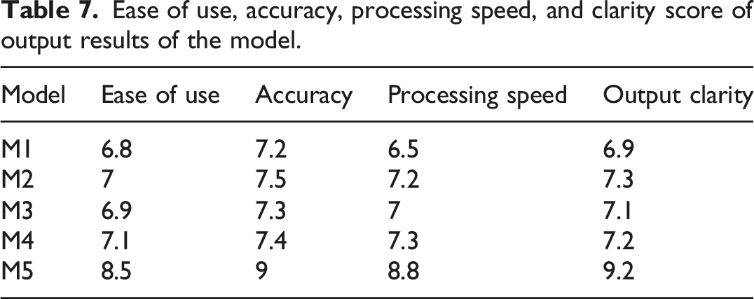
According to the data in Table 7, M1 scored only 6.8, 7.2, 6.5, and 6.9 in terms of usability, accuracy, processing speed, and clarity of output results, indicating significant shortcomings in user experience and performance. Although M2, M3, and M4 each have their own advantages, overall they are still inferior to M5. M5 achieved high scores of 8.5, 9.0, 8.8, and 9.2 in these four aspects, far exceeding other models.

According to the data in Table 7, the overall satisfaction average score for each model can be calculated, as shown in Figure 6.

Figure 6.

Overall satisfaction score of the model.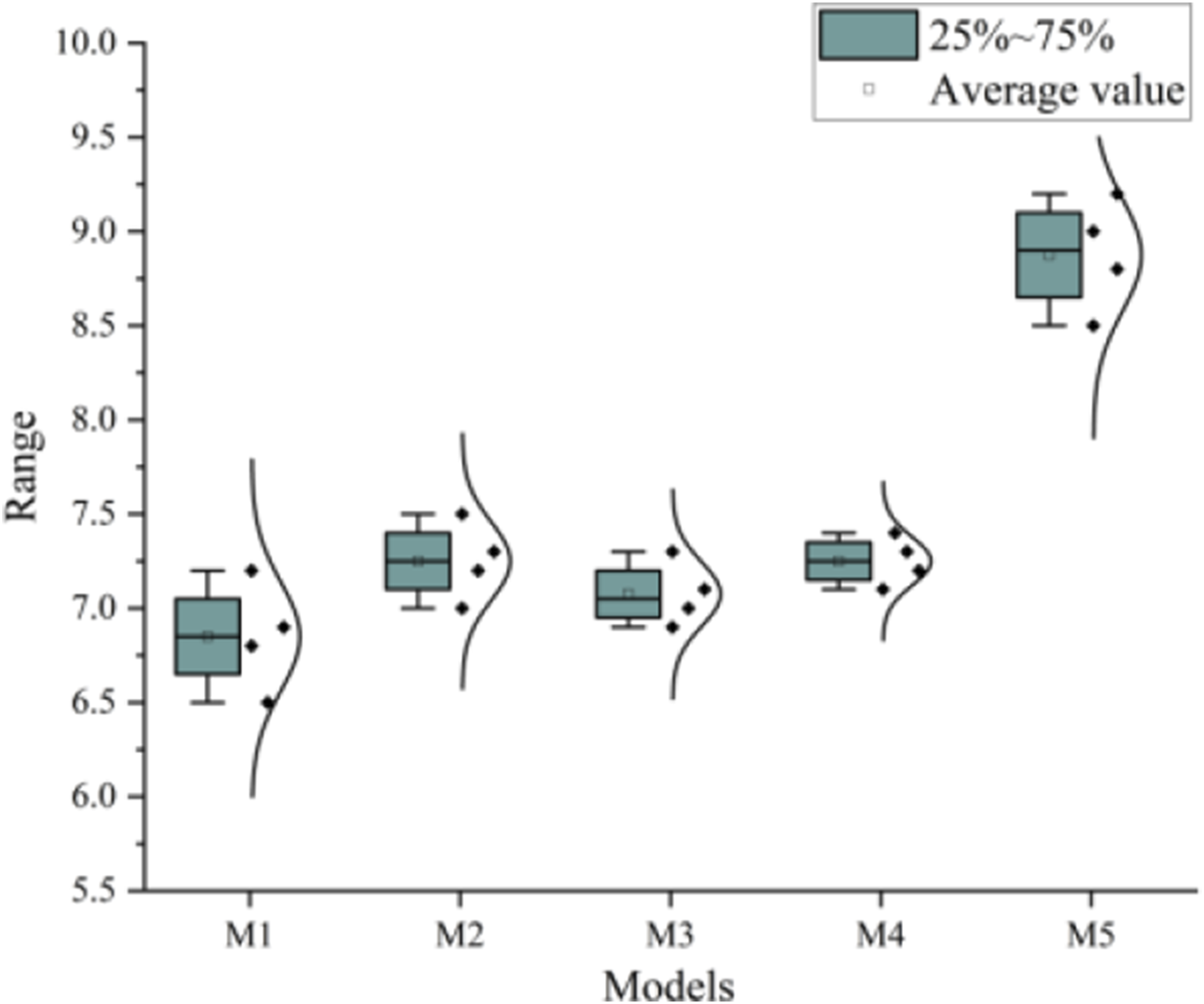

In Figure 6, M5 still has the highest average satisfaction score, which fully demonstrates the superiority of LSTM algorithm in handling English text sentiment analysis tasks and provides strong empirical support for improving user satisfaction of sentiment analysis models.

Conclusions

This article mainly aims to significantly improve the performance of English text sentiment analysis by applying the LSTM algorithm, especially in dealing with complex texts and long-term dependency relationships. By carefully designing preprocessing steps, combining Word2Vec and TF-IDF technologies for feature extraction, and introducing positional encoding, models applying LSTM algorithm can gain a deeper understanding of the emotional color of language. The experimental results show that the accuracy of the model is much higher than other benchmark models on different test sets. In terms of processing speed, the LSTM model has the shortest processing time in the three stages of dataset preprocessing, feature vectorization, and sentiment classification. However, there is still room for further improvement in research. The performance of the model in handling extreme emotions or satirical statements still needs to be optimized. Additionally, there are still issues that need to be addressed, including improving the accuracy of extreme emotion recognition, handling ironic statements, capturing subtle emotional differences, and optimizing model efficiency. The next research plan includes applying attention mechanisms, combining sentiment lexicons and semantic analysis, exploring new models, conducting cross-domain sentiment analysis, and model interpretability research. Future work can explore more complex deep learning models to further enhance the ability to capture subtle differences in text emotions.

Footnotes

Funding

The author received no financial support for the research, authorship, and/or publication of this article.

Declaration of conflicting interests

The author declared no potential conflicts of interest with respect to the research, authorship, and/or publication of this article.

References

Cen

Zhang

Zheng

. Sentiment analysis using deep learning approach. J Artif Intell 2020; 2(1): 17–27.

Hung

Alias

. Beyond sentiment analysis: a review of recent trends in text based sentiment analysis and emotion detection. J Adv Comput Intell Intell Inf 2023; 27(1): 84–95.

Marlina

Tri Basuki

Mohd

, et al. Sentiment analysis on natural skincare products. J Data Sci 2022; 2022(12): 1–17.

Rice

Zorn

. Corpus-based dictionaries for sentiment analysis of specialized vocabularies. Political Sci Res Methods 2021; 9(1): 20–35.

Raza

Faizan

Hamza

, et al. Scientific text sentiment analysis using machine learning techniques. Int J Adv Comput Sci Appl 2019; 10(12): 157–165.

Yadav

Vishwakarma

. Sentiment analysis using deep learning architectures: a review. Artif Intell Rev 2020; 53(6): 4335–4385.

Bonta

Kumaresh

Janardhan

. A comprehensive study on lexicon based approaches for sentiment analysis. Asian Journal of Computer Science and Technology 2019; 8(S2): 1–6.

D’Aniello

Gaeta

La Rocca

. KnowMIS-ABSA: an overview and a reference model for applications of sentiment analysis and aspect-based sentiment analysis. Artif Intell Rev 2022; 55(7): 5543–5574.

Hartmann

Heitmann

Siebert

, et al. More than a feeling: accuracy and application of sentiment analysis. Int J Res Market 2023; 40(1): 75–87.

10.

Deng

Zhao

, et al. A novel hybrid short-term load forecasting method of smart grid using MLR and LSTM neural network. IEEE Trans Ind Inf 2020; 17(4): 2443–2452.

11.

Ruwali

Kumar

AJS

Prakash

, et al. Implementation of hybrid deep learning model (LSTM-CNN) for ionospheric TEC forecasting using GPS data. IEEE Geosci Remote Sens Lett 2020; 18(6): 1004–1008.

12.

Rahimzad

Moghaddam Nia

Zolfonoon

, et al. Performance comparison of an LSTM-based deep learning model versus conventional machine learning algorithms for streamflow forecasting. Water Resour Manag 2021; 35(12): 4167–4187.

13.

Tripathi

. Sentiment analysis of Nepali covid19 tweets using nb svm and lstm. J Artif Intell 2021; 3(03): 151–168.

14.

Park

Lee

. Prediction of high turbidity in rivers using LSTM algorithm. J Korean Soc Water Wastewater 2020; 34(1): 35–43.

15.

Kim

Lee

, et al. The prediction of COVID-19 using LSTM algorithms. International Journal of Networked and Distributed Computing 2021; 9(1): 19–24.

16.

Zhang

Chau

Chow

, et al. A novel sequence to sequence data modelling based CNN-LSTM algorithm for three years ahead monthly peak load forecasting. IEEE Trans Power Syst 2023; 39(1): 1932–1947.

17.

Liu

. Wet antenna attenuation model of E-band microwave links based on the LSTM Algorithm. IEEE Antennas Wirel Propag Lett 2020; 19(9): 1586–1590.

18.

ShanYou

Wang

, et al. Prediction of instrumental intensity for a single station using a LSTM neural network. Chin J Geophys 2024; 67(2): 587–599.

19.

Kulkarni

Mundhe

. An application of porters stemming algorithm for text mining in healthcare. Int J Manag IT Eng (IJMIE) 2019; 7(11): 223–228.

20.

Johnson

Murty

Navakanth

. A detailed review on word embedding techniques with emphasis on word2vec. Multimed Tool Appl 2024; 83(13): 37979–38007.

21.

Satish

, et al. Parallelizing word2vec in shared and distributed memory. IEEE Trans Parallel Distr Syst 2019; 30(9): 2090–2100.

22.

Lee

Kim

. A study on Korean language processing using TF-IDF. J Inf Syst 2019; 28(3): 105–121.

23.

Umadevi

. Document comparison based on tf-idf metric. International Research Journal of Engineering and Technology (IRJET) 2020; 7(02): 1546–1550.

24.

, et al. A review of recurrent neural networks: LSTM cells and network architectures. Neural Comput 2019; 31(7): 1235–1270.

25.

Mao

. Deep-convolution-based LSTM network for remaining useful life prediction. IEEE Trans Ind Inf 2020; 17(3): 1658–1667.

26.

Turkoglu

Hanbay

Sengur

. Multi-model LSTM-based convolutional neural networks for detection of apple diseases and pests. J Ambient Intell Hum Comput 2022; 13(7): 3335–3345.

27.

Kehm

Larsen

Sommersel

. Student dropout from universities in Europe: a review of empirical literature. Hungarian Educational Research Journal 2019; 9(2): 147–164.

28.

Nicoletti

. Revisiting the Tinto’s theoretical dropout model. High Educ Stud 2019; 9(3): 52–64.

29.

Vershynin

. Memory capacity of neural networks with threshold and rectified linear unit activations. SIAM Journal on Mathematics of Data Science 2020; 2(4): 1004–1033.

30.

Zhao

Zhong

, et al. Deep residual networks with adaptively parametric rectifier linear units for fault diagnosis. IEEE Trans Ind Electron 2020; 68(3): 2587–2597.

31.

Cartis

Gould

Toint

. Universal regularization methods: varying the power, the smoothness and the accuracy. SIAM J Optim 2019; 29(1): 595–615.

Model	Ease of use	$Accuracy$	Processing speed	Output clarity
M1	6.8	7.2	6.5	6.9
M2	7	7.5	7.2	7.3
M3	6.9	7.3	7	7.1
M4	7.1	7.4	7.3	7.2
M5	8.5	9	8.8	9.2

Model	Ease of use	$Accuracy$	Processing speed	Output clarity
M1	6.8	7.2	6.5	6.9
M2	7	7.5	7.2	7.3
M3	6.9	7.3	7	7.1
M4	7.1	7.4	7.3	7.2
M5	8.5	9	8.8	9.2

Model	Ease of use	$Accuracy$	Processing speed	Output clarity
M1	6.8	7.2	6.5	6.9
M2	7	7.5	7.2	7.3
M3	6.9	7.3	7	7.1
M4	7.1	7.4	7.3	7.2
M5	8.5	9	8.8	9.2