Implementation of instrument recognition based on audio signals using convolutional neural networks

Abstract

The significance of instrument recognition based on audio signals lies in its broad potential across diverse fields such as music education, intelligent technology, and even medical diagnosis. In this study, we focus on tackling the challenges posed by the OpenMIC-2018 (Open Museum Identification Challenge-2018) dataset. Leveraging the powerful nonlinear modeling capabilities of convolutional neural networks (CNNs), the research aims to address common interference factors in instrument recognition, such as background noise, pitch variations, and volume fluctuations during performances. By effectively mitigating these challenges, this approach enhances the accuracy and precision of instrument recognition, offering valuable contributions to both academic research and practical applications. Firstly, FFT (fast Fourier transform) is used to extract MFCC (Mel-frequency cepstral coefficient), chroma, time-domain, and spectral energy from each audio frame. Initial CNN models with 10 different hyperparameters are trained, and the prediction results are merged with the original features. Then, one-dimensional convolutional layers are used for spectral feature convolution operations, and pooling layers are used for downsampling. ReLU (rectified linear unit) is used as the activation function and nonlinearity is applied. Dropout layers are added between convolutional layers and a portion of neurons are randomly set to zero. Next, the learning rate is adjusted based on cross-validation. For multi-label classification tasks, a binary cross-entropy loss is used and parameters are updated through backpropagation algorithm. Finally, a secondary CNN model is used. The merged features are input and the prediction results are obtained. The research results indicate that the innovative method used achieves an average accuracy of 0.92 on OpenMIC-2018, with an accuracy of 0.97 for accordion, flute, and organ, realizing relatively precise instrument recognition.

Keywords

instrument recognition audio signal convolutional neural network fast Fourier transform Mel-frequency cepstral coefficient

Introduction

Instrument recognition is an essential research direction in audio signal processing, with broad application prospects. This technology can help music educators better teach the performance skills of different instruments,¹ and can also be applied in intelligent music synthesis,² information retrieval,³ and medical diagnosis.⁴ However, in practical applications, instrument performance is often affected by environmental factors,^5,6 and factors such as background noise, pitch variation, and volume may affect the signal characteristics of the instrument, thereby reducing recognition stability.^7,8 How to effectively address these factors and improve the accuracy of instrument recognition has become one of the important research topics.

In the past, the main focus was on utilizing various feature extraction methods and classifiers to achieve instrument recognition. Among them, methods based on spectral features are more common.^9,10 By extracting spectral features of audio signals, including power spectral density¹¹ and spectral envelope,¹² classifiers are used to classify different instruments. By mapping audio data to matrix format, Solanki Arun et al.¹³ estimated any number of instruments from audio signals with variable length. Testing was conducted on 16 musical instruments, and Prabavathy et al.¹⁴ fused SVM (support vector machine) and KNN (k-nearest neighbors) to achieve instrument classification. Using only the MFCC of audio data as features, Mahanta Saranga Kingkor et al.¹⁵ successfully classified musical instruments based on ANN (artificial neural network). After training on the FMA dataset, Chillara Snigdha et al.¹⁶ found that the model had high accuracy when only providing spectrograms. Existing methods are usually sensitive to interference factors such as background noise and volume changes, resulting in poor recognition performance in complex environments.^17,18 Some time-domain feature-based methods attempt to achieve instrument recognition by analyzing the time-domain waveform characteristics of audio signals, but they are also subject to severe interference.^19,20 At present, there are still certain limitations and challenges in the practical application of instrument recognition methods.

Some researches have begun to explore improving CNN for instrument recognition. CNN is gradually becoming a popular research topic in instrument recognition due to its excellent feature learning and pattern recognition capabilities.^21,22 Compared to traditional feature extraction methods,^23,24 it has stronger nonlinear modeling ability²⁵ and can better adapt to the environmental interference of different instruments.²⁶ The instrument recognition method using this model has achieved outstanding results when using large-scale datasets and optimizing network structures.^27,28 Sarkar Rajib et al.²⁹ proposed a CNN built around VGGNet (visual geometry group network) to effectively improve instrument recognition performance. By introducing components of residual networks and squeeze excitation networks, Kim et al.³⁰ extended SampleCNN to a more advanced version to distinguish the acoustic characteristics of different instruments. For small sample scenarios lacking labeled datasets, Yagya Raj et al.³¹ trained a one-dimensional CNN-based music sentiment classifier using raw waveform input, with an accuracy of 88.6%. Remzi³² compared the performance of DenseNet, ResNet, and CNN algorithms and found that the CNN model achieved the highest accuracy (99.3%). Joshi et al.³³ demonstrated in their experiment that in instrument classification tasks, the CNN model using Mel spectrograms was superior to using MFCC. However, even the best DCNN (dynamic convolutional neural network) model currently available³⁴ still has a recognition rate of only around 0.85 for the OpenMIC-2018 dataset.³⁵ This article takes the OpenMIC-2018 dataset as a starting point and attempts to further achieve higher accuracy.

This article focuses on using convolutional neural networks (CNN) for instrument recognition and analysis based on audio signals. The audio signals are transformed into frequency-domain signals through fast Fourier transform (FFT), and spectral features are extracted using Mel-frequency cepstral coefficient (MFCC), incorporating processes such as framing, windowing, Fourier transform, Mel filter bank filtering, logarithmic operation, and discrete cosine transform. Both time-domain and frequency-domain features are captured simultaneously. The data is divided into training and validation sets, and multiple CNN models are trained using different hyperparameters. The feature representation is further enhanced by stacking prediction results, followed by secondary training with CNN models.

The CNN models demonstrate high precision in recognizing 20 musical instruments, with an average recognition precision of 0.90 and an overall recognition accuracy of 0.92. The evaluation metrics are strong, with an average AUC of 0.96, an average MAE of 0.005, and a Cohen’s Kappa of 0.85. Additionally, the model achieves impressive results in Top-3, Top-5, and Top-10 accuracy, with scores of 0.88, 0.90, and 0.92, respectively. This research innovatively addresses the challenges of low recognition accuracy and sensitivity to interference in instrument recognition, leading to notable improvements in performance.

Dataset description

OpenMIC-2018 is an open music dataset aimed at promoting research on multi-instrument recognition in the field of music information retrieval (MIR). Its construction combines the advantages of the free music archive (FMA) dataset and AudioSet. FMA is a free music collection that includes the music in various genres and eras. AudioSet is a large and diverse audio event dataset that includes millions of labeled 10-second audio clips. By combining these two datasets, OpenMIC-2018 contains 20,000 audio clips, each labeled with the presence of 20 different instrument categories. More than 2000 researchers have conducted crowdsourcing annotation on fragments, further improving the quality of annotation.

The statistics of the number of annotations for each instrument category are shown in Figure 1. Among them, 20 instruments include accordion, banjo, bass, cello, clarinet, cymbals, drums, flute, guitar, mallet percussion, mandolin, organ, piano, saxophone, synthesizer, trombone, trumpet, ukulele, violin, and voice (the voice here refers to human voice).

Figure 1.

Label distribution of 20 instruments in OpenMIC-2018.

Feature extraction

In the study of instrument recognition, different categories of instruments possess unique acoustic characteristics. Utilizing FFT for spectrum analysis converts audio signals into frequency-domain representations. By using methods such as MFCC, chromaticity characteristics, time, and spectral energy, the differences in frequency, pitch, and amplitude of the instrument are effectively captured. For brass and string instruments, spectral features may exhibit prominent frequency peaks and harmonic structures, whereas woodwind instruments often display more complex frequency distributions and tonal variations. Detailed analysis and extraction of acoustic characteristics for each instrument category can improve the accuracy and robustness of the model in identifying specific instruments, meeting the requirements of practical application scenarios.

Spectral analysis is performed on each audio frame using FFT to convert time-domain signals into frequency-domain signals. By calculating the amplitude and phase information of each frequency component, the representation of the audio signal in the frequency domain is obtained. For an audio frame $x [n]$ with length $N$ , its FFT transformation is represented as:

X (k) = \sum_{n = 0}^{N - 1} x [n] \cdot e^{- j 2 π n k / N}

(1)

Among them, $X (k)$ is the spectral component with a frequency of $f_{k} = \frac{k}{N} f_{s}$ . $f_{s}$ is the sampling rate. $n$ is the sample index in the time-domain. $k$ is the frequency index in the frequency domain. Next, MFCC is used to describe the spectral characteristics of audio signals, which is a feature representation method based on human auditory perception characteristics. It can effectively capture the frequency changes of audio signals and has a good fitting effect on human auditory perception. The calculation steps are as follows:

(a) Framing: audio signals are split into several fixed-length audio frames.

(b) Windowing: a Hanning window is applied to each audio frame to reduce spectrum leakage.

(d) Mel filter bank filtering: the spectrogram is filtered through a set of Mel filters to obtain the Mel spectrogram.

(e) Logarithmic operation: the logarithm of the Mel spectrogram is taken to obtain the logarithmic Mel spectrogram.

(f) Discrete cosine transform: a discrete cosine transform is performed on a logarithmic Mel spectrogram to obtain the MFCC coefficients.

The calculation formula is expressed as:

M F C C_{i} = \sum_{j = 1}^{M} \log (\sum_{k = 1}^{N} | X (k) |^{2} H_{m} (k) \cos [\frac{π i}{M} (k - 0.5)])

(2)

Here,

H_{m} (k)

is the frequency response of the

m

-th Mel filter;

M

represents the number of MFCC coefficients;

N

represents the number of FFT points;

i

represents the MFCC coefficient index.

Chroma features are extracted to describe the pitch information of audio signals. Chroma feature is a method of describing the pitch characteristics of music and sound. The audio signals are mapped to the scale space of music, and the changes in pitch of audio signals are captured. The calculation of chroma features is represented as:

C_{i} = \sum_{k = 1}^{N} | X (k) |^{2} G_{i} (k)

(3)

Among them, $G_{i} (k)$ represents the frequency response of the $i$ -th chroma channel, and $i$ represents the chroma channel index. Additionally, time-domain and frequency-domain features are extracted to describe the time-domain and frequency-domain characteristics of audio signals. The time-domain features mainly include the time-domain energy of the audio signal, and the frequency-domain features mainly include the spectral energy of the audio signal. Their calculation is as follows:

E_{t} = \sum_{n = 1}^{N} | x (n) |^{2}

(4)

E_{f} = \sum_{f = 1}^{F} | X (f) |^{2}

(5)

Here, $x (n)$ represents the discrete sampling value of the audio signal in the time-domain, where $n$ represents the index of the sampling points. $X (f)$ represents the spectral representation of audio signals in the frequency domain, where $f$ represents the frequency. To intuitively showcase the characteristics of audio signals, the article provides the visual representation shown in Figure 2, offering an in-depth analysis of the intrinsic structure of a single audio sample. Figure 2 shows the results of feature extraction on a single sample.

Figure 2.

Audio signal feature extraction in a single sample. (a) MFCC; (b) chroma; (c) audio signal; and (d) frequency-domain energy.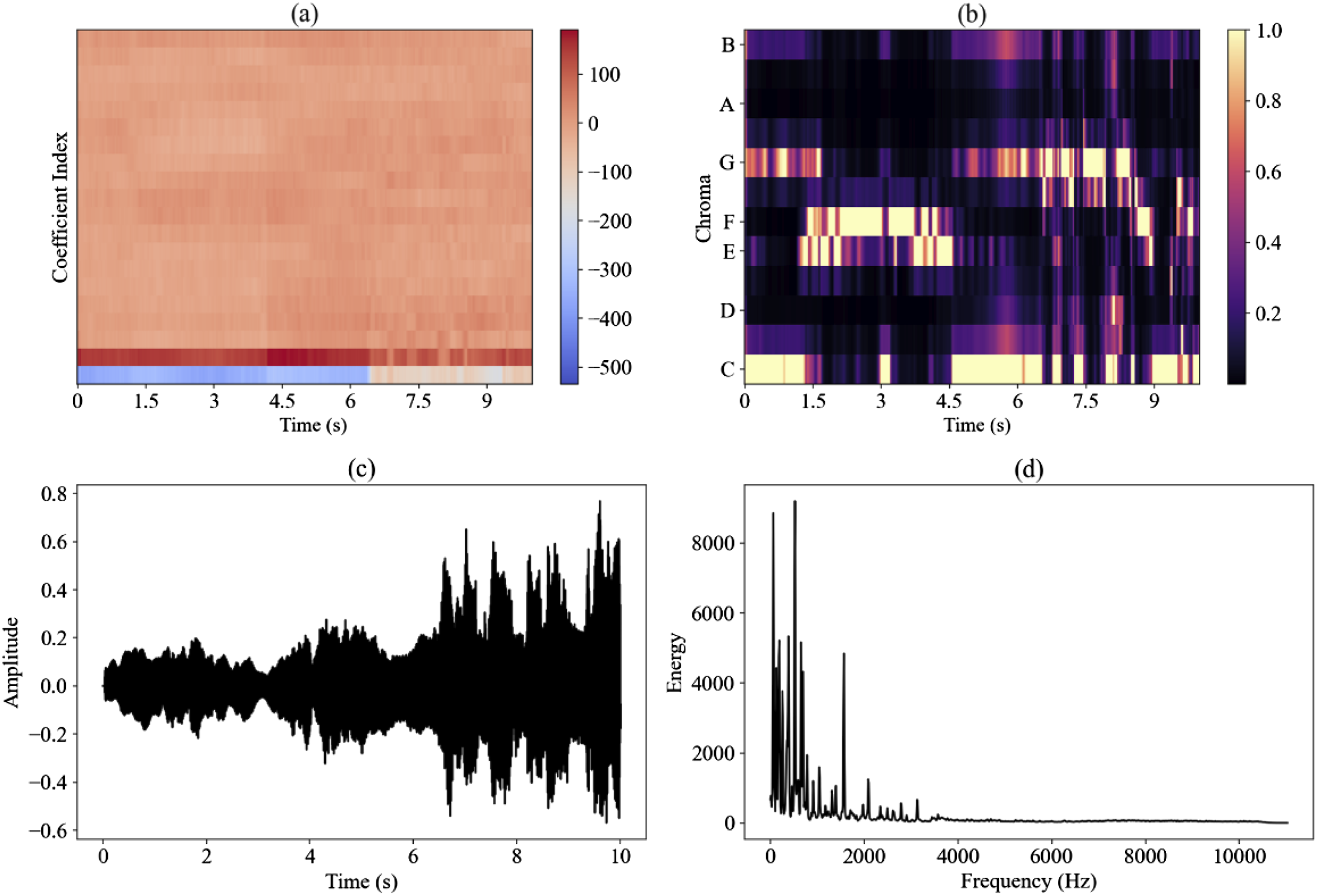

In the Mel-frequency cepstral coefficients shown in Figure 2(a), the horizontal axis represents time (in seconds) and the vertical axis represents the MFCC coefficient index. The data is an MFCC coefficient matrix, where each element represents the MFCC value of the audio signal at a specific time point, reflecting the spectral characteristics of the audio signal. Figure 2(b) shows the chroma features obtained by calculation, where the horizontal axis represents time (in seconds) and the vertical axis represents pitch index. The data is represented as a chroma feature matrix, where each element represents the pitch intensity of the audio signal at a specific time point. Figure 2(c) shows the audio signal, with the horizontal axis representing time (in seconds) and the vertical axis representing the amplitude of the audio signal. The data is the variation of the amplitude of an audio signal over time. Figure 2(d) shows the frequency-domain energy, with the horizontal axis representing frequency (in hertz) and the vertical axis representing energy values. The data is a vector of the frequency-domain energy spectrum, where each element represents the energy of the audio signal at a specific frequency.

In addition to traditional MFCC and chroma features, this article also attempts to extract more types of audio features such as pitch, harmony, spectral centroid, spectral rolloff, and zero crossing rate to enrich the feature set. FFT is used to perform spectrum analysis on each audio frame, transforming the audio signals into frequency-domain representations and further extracting amplitude and phase information of frequency components. MFCC is adopted to describe the spectral characteristics of the audio signals, capturing frequency variations through Mel-filter bank filtering, logarithmic operations, and discrete cosine transformation. Chroma features capture variations in musical pitch, and spectral and temporal energy describe the temporal and frequency-domain characteristics of the audio signals. The application of these expanded features enhances the model’s understanding and analysis capabilities of audio signal features, facilitating more precise instrument recognition and analysis.

The spectral centroid is the centroid position of a spectrum, reflecting the average frequency and describing the pitch of sound. Spectral rolloff is the frequency point below which 85% of the total energy of the spectrum is located, often used to measure high-frequency content and clarity of the spectrum. Zero crossing rate is the number of times a signal waveform crosses the zero axis on the time axis, reflecting the signal’s rate of change and frequency components.

This article analyzes the contribution of each feature to instrument recognition accuracy through statistical methods, information gain, and SHAP feature importance assessment tools. The importance of extracting features is evaluated to eliminate redundant or irrelevant features, and key features that distinguish different instruments are identified. This optimization improves the quality and efficiency of the model’s input features. Feature selection ensures that the model focuses on capturing the most discriminative audio features, thereby improving the stability of instrument recognition.

Feature stacking and fusion

Using CNN to process variable-length audio inputs involves preprocessing different-length audio segments dynamically to ensure uniform input format. In model design, applying one-dimensional convolutional layers and global pooling layers replaces fixed-size pooling operations, accepting variable-length inputs and generating fixed-length feature representations. Incrementally increasing convolutional kernel sizes and strides helps effectively capture local and global features within audio segments.

To improve the accuracy of instrument recognition, this article innovatively adopts feature stacking and fusion methods, and Figure 3 shows the overall process.

Figure 3.

Process of feature stacking.

Features are extracted from the raw data and the set is divided into a training set and a validation set. Initial CNN models are trained with different hyperparameters on the training set. A basic model with multiple different parameter settings (learning rate, convolutional kernel size, and number of convolutional layers) is established to increase model diversity and generalization ability. After each initial CNN model is trained, prediction results are generated on the validation set, which are merged with the original features as new features. The original feature expression ability is enriched based on stacking methods. These features are input into a secondary CNN model for training, further exploring feature correlations to better capture instrument features in audio signals. Table 1 shows the parameters and accuracy results of initial CNN constructed in this article for the instrument accordion.

Table 1.

Parameters and accuracy results of the initial CNN model.

Initial CNN model	Learning rate	Kernel size	Convolutional layers	Accuracy (%)
Model 1	0.001	3 × 3	2	85.2
Model 2	0.0005	5 × 5	3	77.6
Model 3	0.001	7 × 7	4	88.3
Model 4	0.0007	3 × 3	3	76.5
Model 5	0.001	5 × 5	4	80.4
Model 6	0.0006	7 × 7	2	86.8
Model 7	0.0008	3 × 3	4	77.9
Model 8	0.001	5 × 5	2	88.1
Model 9	0.0005	7 × 7	3	76.7
Model 10	0.0009	3 × 3	2	77.3

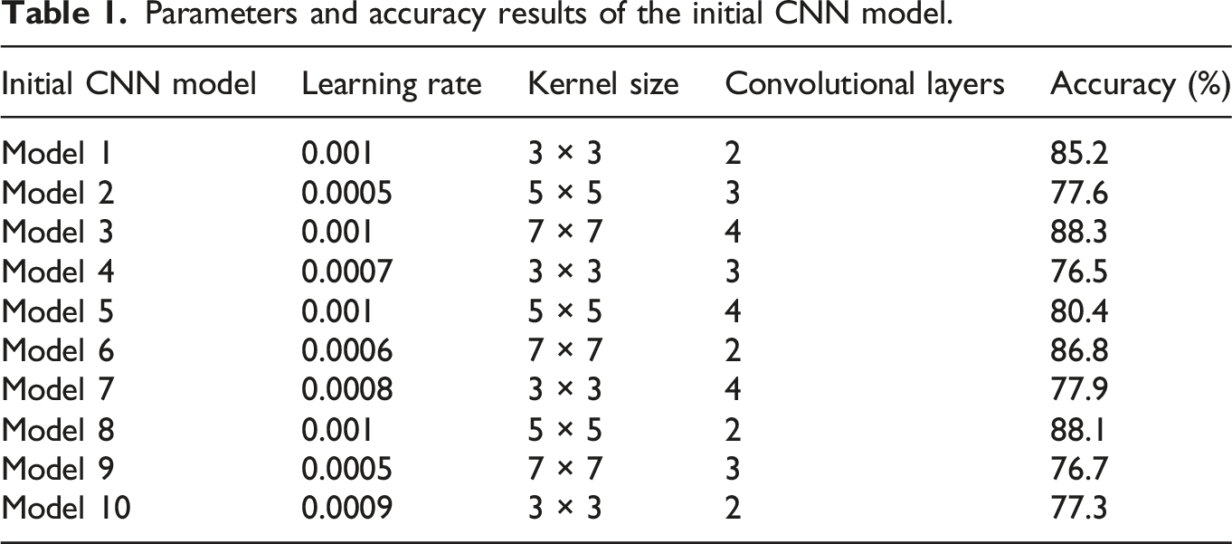
The model design covers different learning rate settings from 0.0005 to 0.001, as well as various convolution kernel sizes, including 3 × 3, 5 × 5, and 7 × 7. In addition, the number of convolutional layers varies from 2 to 4, exploring the impact of different network depths on recognition performance. Although the learning rates of models 2 and 10 are 0.0005 and 0.0009, respectively, and both use a 3 × 3 kernel size, their accuracies reach 77.6% and 77.3%, respectively, indicating a complex interaction between model depth and learning rate. For models 3 and 8, both achieve an accuracy of over 88%. Model 3 uses a larger 7 × 7 kernel and 4 convolutional layers, achieving the highest accuracy of 88.3%. Model 8 achieves an accuracy of 88.1% using a smaller 5 × 5 kernel and only 2 convolutional layers. This indicates that under specific conditions, increasing the model depth appropriately or using larger convolution kernels can significantly improve the effectiveness of instrument recognition.

To further optimize the learning rate adjustment during the training process, the article applies cosine annealing and step learning rate strategies. The cosine annealing strategy periodically lowers the learning rate during training, helping the model to better jump between local optima and improving overall performance. The learning rate decreases gradually according to the cosine function’s period, enabling the model to converge more robustly in the later stages of training. On the other hand, the step learning rate strategy reduces the learning rate by a fixed proportion every certain number of epochs during training, allowing the model to adapt to different learning rate requirements at various training stages, effectively addressing the learning rate adjustment issue. Combining these two learning rate scheduling strategies further improves the model’s performance on the OpenMIC-2018 dataset, significantly enhancing the model’s training stability.

Table 1 shows the accuracy of initial CNN recognition for instrument accordion in 10 different model parameter combinations. The same applies to other musical instruments. The accuracy calculation results of 10 initial models are stacked into 20 instrument features. The average and standard deviation of accuracy for recognizing different musical instruments (with 10 model parameters) are shown in Figure 4.

Figure 4.

Average and standard deviation of accuracy for recognizing different musical instruments using 10 types of initial CNN.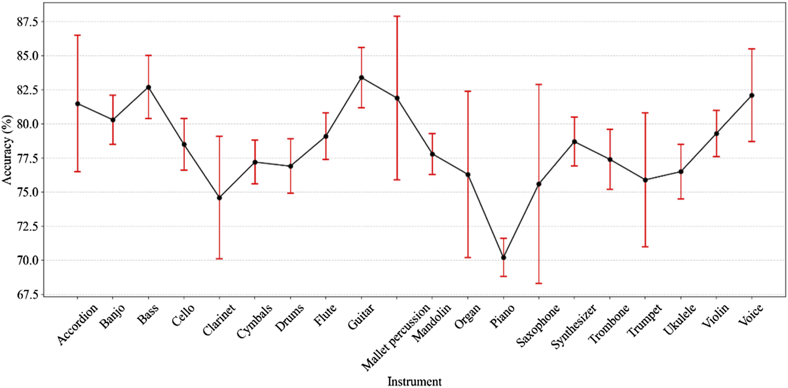

According to Figure 4, the average accuracy of 10 types of initial CNN for recognizing different instruments ranges from 0.70 to 0.84. Meanwhile, there is a significant fluctuation in accuracy calculation for some instruments under different parameters (the standard deviation calculation results are marked with red error lines). The CNN model needs to be further optimized based on the characteristics of audio data.

Model construction, training, and optimization

This article presents an innovative improvement of convolutional neural network (CNN) based on audio signals in instrument recognition. In this article, feature stacking and fusion methods are applied to train initial CNN models with different hyperparameters, and the predictions of these models are combined with the original features to enrich feature representation and improve recognition accuracy. In terms of model structure, one-dimensional convolutional layers are applied to the spectral features of audio signals, and downsampling is performed through pooling layers to reduce feature dimensionality and improve computational efficiency. ReLU activation function is applied between convolutional layers to enhance the nonlinear expression ability of the model, and dropout layers are added to prevent overfitting, thereby improving the stability and robustness of the model. An attention mechanism is applied to the model to dynamically adjust the weights of different time scales in audio signals. Through this attention mechanism, the model can automatically focus on more important segments within the audio signals, thereby effectively capturing the characteristics of different musical instruments.

CNN is used as the main model framework, and one-dimensional convolutional layers are used to convolve the spectral features of audio signals. The spectral characteristics of the input audio signal are represented as $X$ , and the convolution operation is represented as:

Y [i] = \sum_{j = 0}^{k - 1} X [i + j] \cdot W [j] + b

(6)

Here, $Y$ represents the convolutional feature; $W$ represents a convolutional kernel; $b$ represents the bias term; $k$ is the size of the convolutional kernel. An attention mechanism is applied to dynamically adjust the weights of different time scales. Through attention mechanism, the model can automatically focus on the more important parts of the audio signal, thus more effectively capturing the features of different instruments. After convolution and pooling operations, the attention layer is used to calculate the weights for each time period. These weights are dynamically adjusted based on the context of the audio signal, ensuring that the model pays higher attention to key time points. Pooling layers are used for downsampling operations to reduce feature dimensions and improve computational efficiency.

Z [i] = \max (Y [i \times s : (i + 1) \times s])

(7)

Among them, $Z$ is the pooled feature, and $s$ is the pooled window size. To enhance the model’s expressive power, ReLU is applied as the activation function after the convolutional layer to introduce nonlinear factors. The negative part is set to zero while retaining the positive part. Dropout layers are added between convolutional layers to prevent model overfitting, and model complexity is reduced by randomly zeroing a portion of neurons.

To adjust the model learning rate, a 10-fold cross-validation method is adopted, and multiple training and validation are conducted on different subsets of the training data. The process is shown in Figure 5.

Figure 5.

Adjustment of the learning rate of the model.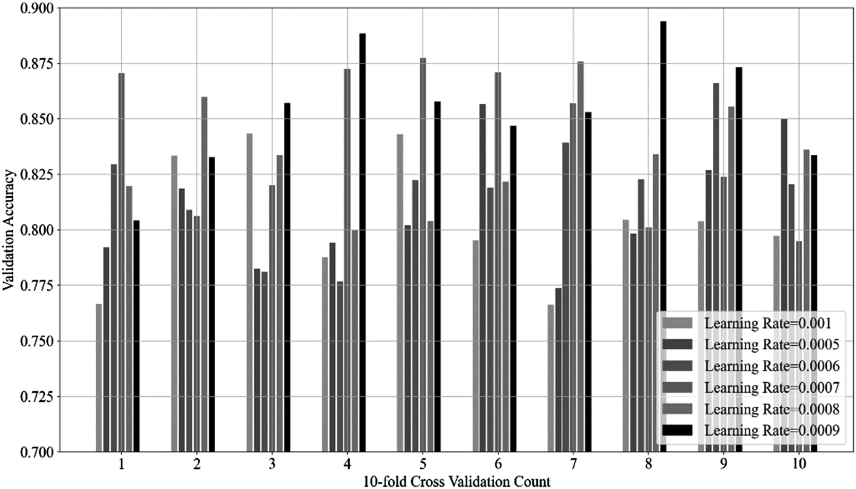

Figure 5 shows the model’s performance across different learning rates in each fold of cross-validation. The accuracy fluctuates with changes in the learning rate. In the first fold, the highest accuracy of 0.87 is achieved with a learning rate of 0.0007, while other learning rates yield slightly lower performance. Similarly, in the fourth fold, a learning rate of 0.0009 results in the highest accuracy of 0.89, the best among all tested learning rates in that fold. However, the optimal learning rate varies across folds; in the fifth fold, the best learning rate is 0.0007, with an accuracy of 0.88. For specific data splits, there is an optimal learning rate that maximizes model performance. After analyzing the average performance of all folds, it is found that learning rates of 0.0007 and 0.0009 typically provide higher accuracy, indicating that they are better choices for the entire dataset.

For multi-label classification tasks, this article uses a binary cross-entropy loss function:

L (y, \hat{y}) = - \frac{1}{N} \sum_{i = 1}^{N} \sum_{j = 1}^{M} [y_{i j} \log ({\hat{y}}_{i j}) + (1 - y_{i j}) \log (1 - {\hat{y}}_{i j})]

(8)

Here, $y_{i j}$ represents the true label and ${\hat{y}}_{i j}$ represents the predicted value of the model. $N$ represents the number of samples, and $M$ represents the number of labels. The gradient of the loss function on the model parameters is computed, the parameters are adjusted in the opposite direction of the gradient, so that the predicted results of the model gradually approach the true situation. The update rule is expressed as:

θ_{t + 1} = θ_{t} - η \nabla_{θ} L (θ)

(9)

Among them, $θ$ is the model parameter; $\nabla$ is the learning rate; $L (θ)$ is the loss function. By introducing Dropout layers between convolutional layers, a portion of neurons are randomly zeroed, thereby reducing the complexity of the neural network: ${\hat{y}}_{i j} = γ \cdot y_{i j} \cdot r$ . Here $r$ is a random variable that follows a Bernoulli distribution, and $γ$ is the retention rate. Simultaneously, to accelerate model training and enhance performance, this article utilizes the RMSprop optimization algorithm. RMSprop dynamically adjusts the learning rate for each parameter by applying an exponentially weighted moving average to the squared gradients of each parameter. This approach maintains stable gradient updates during training, preventing instability caused by excessively large or small learning rates. By continuously adjusting the initial learning rate and decay factor of RMSprop, the optimal parameter settings for the model’s performance on the OpenMIC-2018 dataset are identified. Finally, a secondary CNN model is used to train the merged features and obtain the final prediction result. Figure 6 shows the the overall process.

Figure 6.

Training process of CNN model.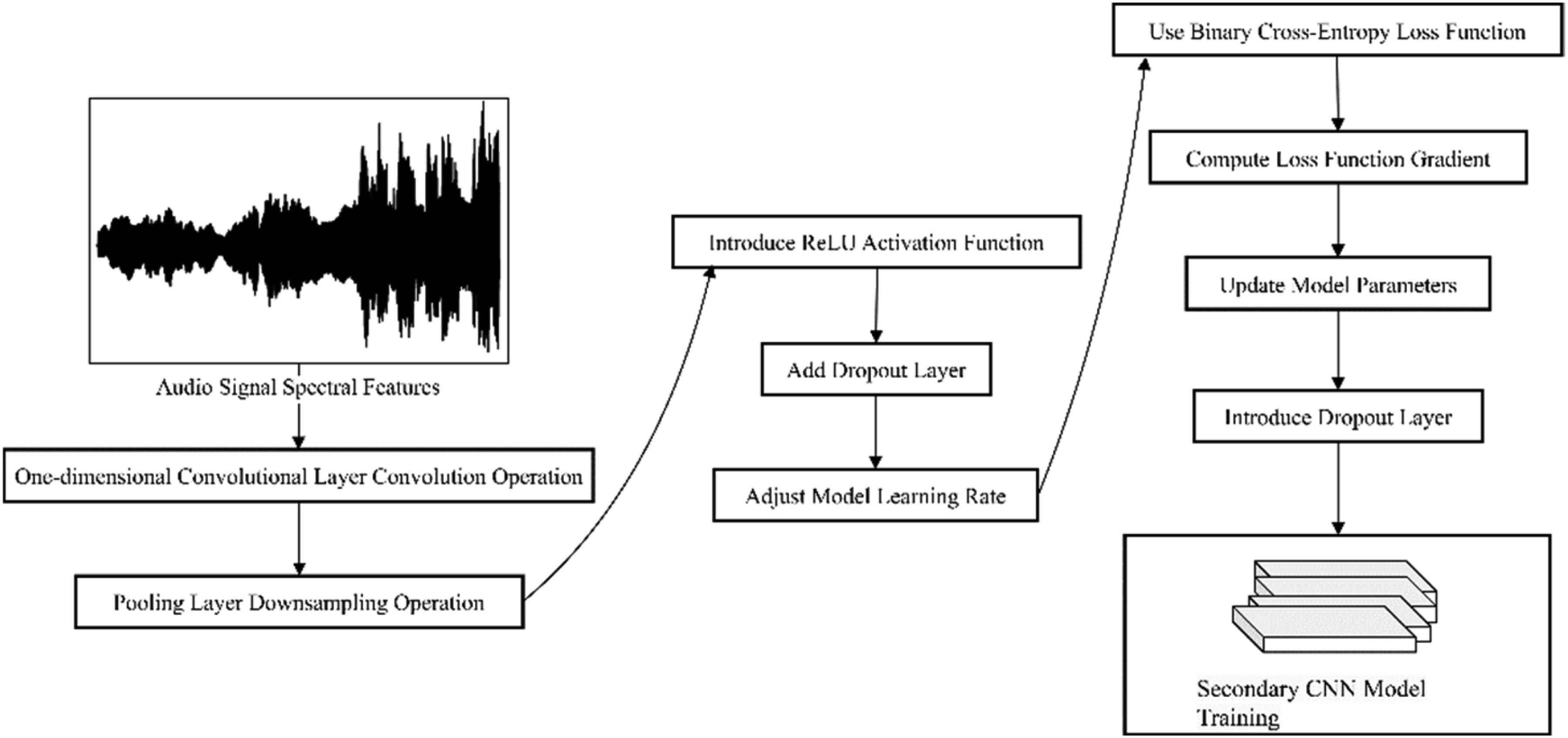

To prevent model overfitting and improve generalization, this article applies an Early Stopping strategy. During training, if the performance on the validation set does not improve after a certain number of iterations, the training process is terminated early. This helps avoid overfitting to the training data, resulting in better performance in practical applications.

Results of model recognition

In the experimental setup, the challenging OpenMIC-2018 dataset is used for musical instrument audio sample analysis. Audio signals are transformed using fast Fourier transform (FFT) and features are extracted, including Mel-frequency cepstral coefficient (MFCC), chroma, time-domain features, and spectral energy. Model training involves 10 CNN models with different hyperparameters. Feature fusion combines prediction results with original features, using 1D convolutional layers and pooling layers for processing. The ReLU activation function is used, and dropout layers are added between convolutional layers to reduce overfitting. Learning rate adjustments are based on cross-validation. For the multi-label classification task, binary cross-entropy loss is used, with parameters updated through backpropagation. Further training is conducted using a secondary CNN model. Parameter configuration includes 1D convolutional layers, ReLU activation function, dropout layers, and binary cross-entropy loss. Evaluation metrics cover average precision, AUC, mean absolute error (MAE), and Cohen’s Kappa. Feature importance is assessed using statistical methods, information gain, and SHAP tools. Feature stacking and fusion involve combining prediction results from multiple models as new feature inputs for the secondary CNN model.

For instrument recognition tasks, based on precision, the performance of CNN models in recognizing multiple instruments is reflected, that is, the proportion of audio predicted to be a certain instrument that truly is the instrument. Meanwhile, the accuracy of the model for each category is calculated, as shown in Figure 7.

Figure 7.

Precision and accuracy of CNN in recognizing 20 musical instruments.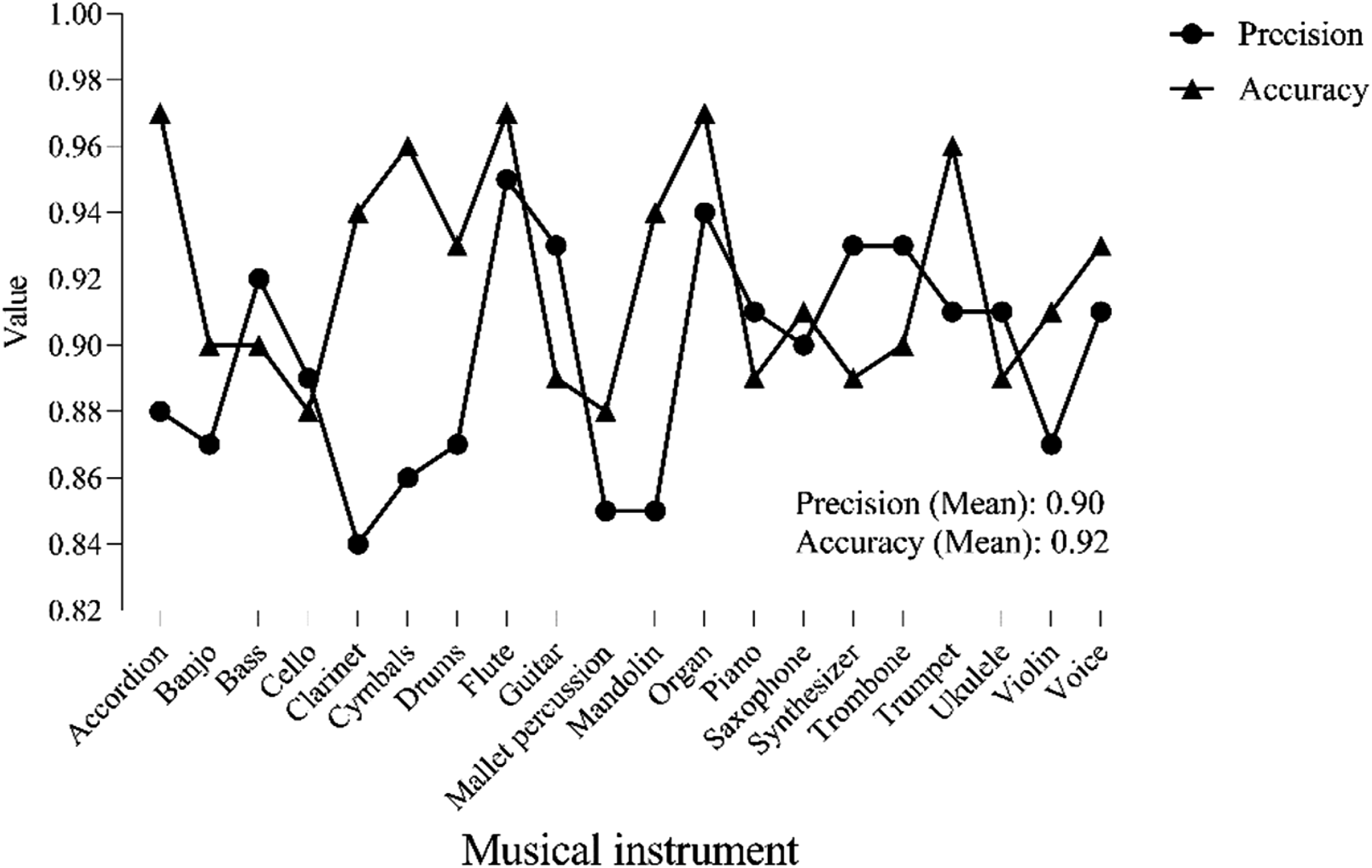

As shown in Figure 7, the highest precision of CNN for recognizing 20 musical instruments is flute (0.95), and the lowest is clarinet (0.84), with an average precision of is 0.90. The instruments with the highest recognition accuracy are accordion, flute, and organ (all 0.97), while the lowest are cello and mallet percussion (all 0.88), with an average accuracy of 0.92. For a single instrument, the CNN model under the improved scheme in this article achieves relatively precise recognition performance. True Skill Statistics (TSS) is further used to consider the sensitivity and specificity of CNN models, and the difference between true positive and true negative rates is calculated to evaluate performance. At the same time, based on Matthews correlation coefficient (MCC), the overall performance of the model is evaluated under imbalanced samples of different categories, taking into account true positive, true negative, false positive, and false negative. The MCC integrates recall and F1 score in its calculation process: MCC considers TP and FN, indirectly reflecting the model’s ability to recall positives. Although MCC does not directly compute the F1 score, it provides a comprehensive assessment similar to the F1 score by integrating TP, TN, FP, and FN, as the F1 score is also based on these metrics. Figure 8 shows the results.

Figure 8.

TSS and MCC of CNN in recognizing 20 musical instruments.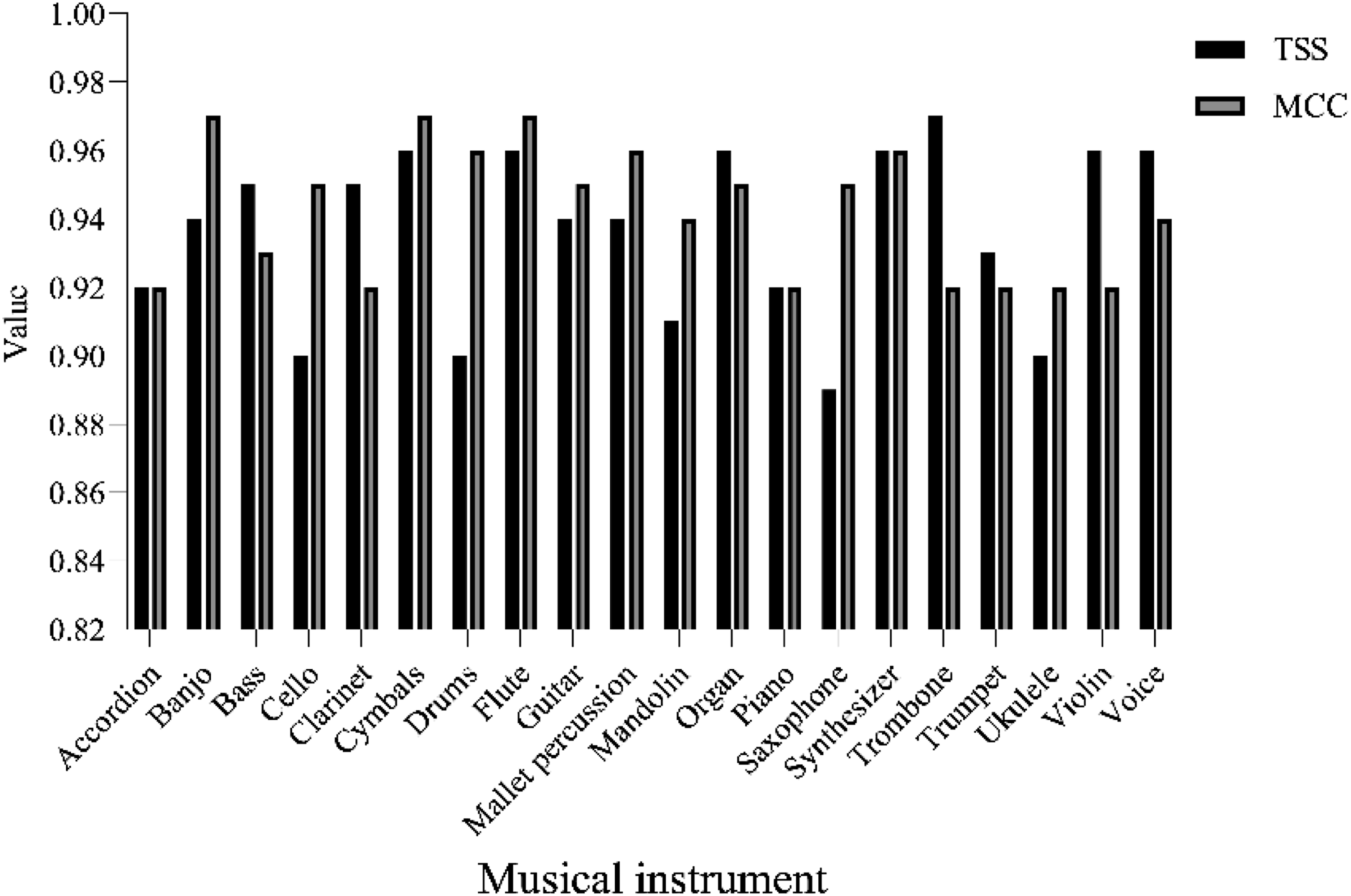

According to the TSS and MCC data shown in Figure 8, the CNN model shows a relatively high level of recognition performance for 20 musical instruments as a whole. The TSS and MCC values of most instrument categories are close to or exceed 0.90, and the model achieves good performance in sensitivity and specificity. Taking the instrument cymbals as an example, its TSS is 0.96 and MCC is 0.97. The model has high sensitivity and specificity in recognizing cymbals, and overall shows high performance under the comprehensive consideration of true positive, true negative, false positive, and false negative.

By conducting an in-depth analysis of the misclassified samples, the limitations of the model under specific conditions can be observed. From the TSS and MCC metrics shown in Figure 8, it is evident that despite the high accuracy in recognizing most instruments, the performance for instruments like “Saxophone” and “Ukulele” is somewhat lacking. This reflects the model’s shortcomings in handling instruments with similar acoustic features. This issue arises from the uneven distribution of samples in the training dataset or the failure to fully capture the unique attributes of these instruments during feature extraction. To address this problem, the article increases the number of training samples for “Saxophone” and “Ukulele,” particularly those with complex background noise and timbral variations, to enhance the model’s understanding and differentiation of these instruments’ unique sounds. On the algorithmic level, attention mechanisms and more complex convolutional layer structures are applied to improve the model’s sensitivity to subtle audio features.

The data shown in Figure 8 demonstrates the effectiveness and robustness of the CNN model in audio signal instrument recognition tasks. The model proposed in this article is further compared with FCNN (fully connected neural network), random forest (RF), and LightGBM (light gradient boosting machine), and the performance of the classifiers is evaluated by plotting the relationship between true positive rate and false positive rate. FCNN is a neural network where each neuron is connected to every neuron in the next layer, suitable for general pattern recognition tasks; RF is an ensemble learning method that uses multiple decision trees to improve prediction accuracy and control overfitting; LightGBM is a fast and efficient gradient boosting framework that uses tree-based learning algorithms, optimized for performance and scalability. Both ROC (receiver operating characteristic) and corresponding AUC (area under curve) values are displayed as shown in Figure 9.

Figure 9.

ROC and AUC of each model in recognizing 20 musical instruments. (a) CNN; (b) FCNN; (c) RF; and (d) LightGBM.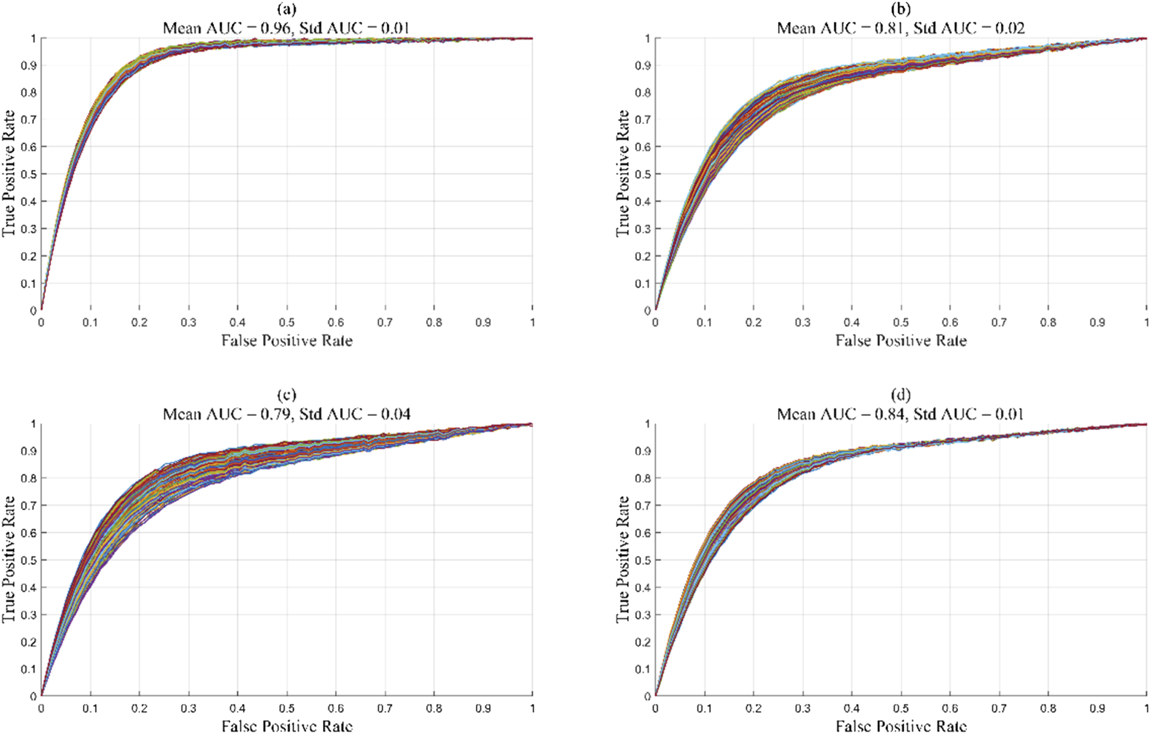

Figure 9(a) and (d) show the ROC curves and corresponding AUC average and standard deviation calculations for binary recognition of 20 musical instruments using four types of models. It can be observed that with the adopted feature stacking method, the CNN model achieves better classification performance compared to other models. Its ROC curve is closer to the upper left corner, and the difference between the curves is small, indicating that the model is relatively stable in the recognition of different instruments. The CNN model achieves a mean AUC of 0.96 (standard deviation/Std = 0.01), 0.81 (Std = 0.02) of FCNN, 0.79 (Std = 0.04) of RF, and 0.84 (Std = 0.01) for LightGBM in recognizing 20 instruments.

The CNN model performs well in audio signal instrument recognition tasks because it can effectively capture the spectral and temporal features of audio signals, and has local feature learning and translation invariance. In contrast, FCNN lacks sufficient extraction of nonlinear features; RF cannot fully utilize the timing information of audio signals; LightGBM has weak recognition ability for spectral features, resulting in poor performance. Based on mean absolute error (MAE), the accuracy of each model in predicting instrument attributes is evaluated, and Table 2 shows the results.

Table 2.

MAE of prediction of 20 types of musical instruments by various models.

Musical instrument	CNN	FCNN	RF	LightGBM
Accordion	0.006	0.01	0.026	0.007
Banjo	0.005	0.009	0.023	0.007
Bass	0.005	0.012	0.024	0.014
Cello	0.005	0.011	0.014	0.006
Clarinet	0.005	0.012	0.013	0.012
Cymbals	0.005	0.012	0.013	0.014
Drums	0.006	0.012	0.013	0.01
Flute	0.007	0.014	0.006	0.008
Guitar	0.004	0.014	0.024	0.007
Mallet percussion	0.003	0.008	0.013	0.006
Mandolin	0.003	0.013	0.01	0.01
Organ	0.006	0.013	0.015	0.009
Piano	0.004	0.008	0.009	0.009
Saxophone	0.006	0.008	0.013	0.012
Synthesizer	0.004	0.01	0.017	0.006
Trombone	0.004	0.015	0.015	0.008
Trumpet	0.007	0.01	0.007	0.012
Ukulele	0.003	0.014	0.008	0.006
Violin	0.007	0.012	0.008	0.007
Voice	0.004	0.015	0.023	0.013
Mean	0.005	0.012	0.015	0.009

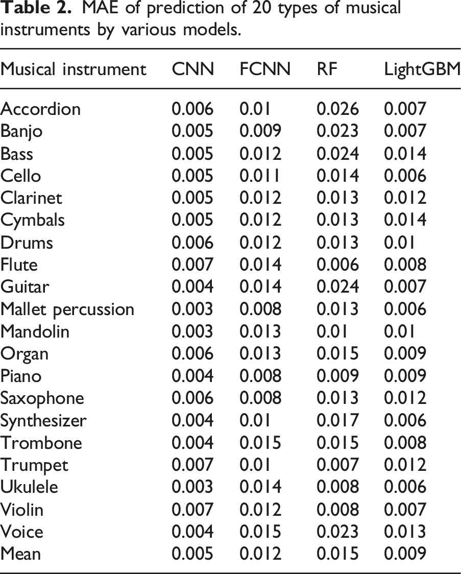
Delving into the model’s sensitivity to different audio features is key to understanding its recognition performance. As shown in Table 2, the CNN model demonstrates exceptional accuracy in predicting instrument attributes, with an average MAE of only 0.005, significantly outperforming fully connected neural networks (FCNN), random forests (RF), and LightGBM models. The results indicate that the CNN model has a keen perception of the spectral and time-domain characteristics of audio signals, achieving recognition accuracy as low as 0.006 to 0.007 MAE for instruments with complex timbral structures such as accordion, flute, and organ, showcasing its high sensitivity to subtle tonal differences. The CNN model also performs excellently on percussive instruments and small plucked instruments like mallet percussion and ukulele, with MAE as low as 0.003, indicating its capability to capture features of both sustained tones and short syllables and rhythmic patterns effectively. In contrast, other models like FCNN, RF, and LightGBM exhibit MAE ranging from 0.008 to 0.024 when handling these instruments, highlighting their limitations in extracting transient and rhythmic information. The article provides valuable insights for future research. On one hand, enhancing the CNN model’s ability to recognize instruments with similar timbres, such as saxophone and clarinet, can further improve its generalization performance. On the other hand, exploring how to enable non-CNN models (like LightGBM) to utilize the time series information of audio more effectively is a worthwhile research direction.

Further evaluation is conducted on the bias and stability of each model in instrument prediction, using mean square error (MSE) and root mean square error (RMSE) as indicators. Table 3 shows the results.

Table 3.

RMSE and MSE of prediction of 20 types of musical instruments by various models.

Evaluation indicators		CNN	FCNN	RF	LightGBM
MSE	Mean	0.005	0.017	0.018	0.008
MSE	Std	0.0005	0.001	0.0007	0.0004
RMSE	Mean	0.072	0.128	0.131	0.088
RMSE	Std	0.001	0.0021	0.012	0.0009

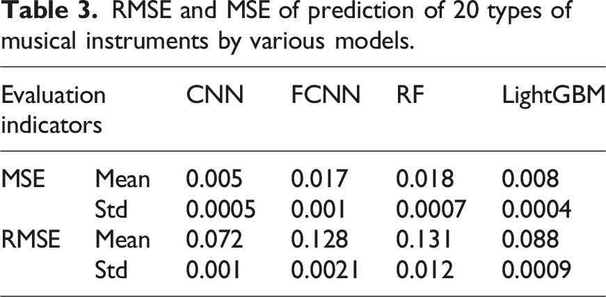
According to Table 3, the CNN model achieves the best prediction accuracy in both MSE and RMSE indicators, with mean values of 0.005 and 0.072, respectively, and relatively small standard deviations, indicating high model stability. The mean values of FCNN and LightGBM models are slightly higher under various indicators, and the standard deviation is relatively large, indicating that the stability of the prediction results is relatively poor. The RF model performs the worst in the RMSE index, with a mean of 0.131 and a standard deviation of 0.012, indicating significant prediction errors. The CNN model has higher accuracy and stability in predicting instrument attributes compared to other models, making it suitable for this task application scenario.

Evaluation results indicate that the CNN model effectively overcomes background noise, volume changes, and other interference factors when processing audio signals, demonstrating robust accuracy. However, the model may still encounter recognition errors when dealing with subtle timbral differences of certain instruments or extreme noise environments. Future research could focus on enhancing the model’s adaptability to complex audio environments by incorporating more diverse training data, covering a wider range of noise types and volume levels, to improve the model’s generalization performance and more precisely capture the nuanced variations in instrument timbre.

Although the Inception module and Transformer model perform well in tasks such as image recognition and natural language processing, their application in audio signal processing is still not very mature. Therefore, this article does not compare the model with them, but rather focuses on comparing it with traditional machine learning models such as FCNN, RF, and LightGBM to more intuitively demonstrate the advantages of convolutional neural networks in multi-label classification tasks. Regarding the performance of the model in multi-label classification problems, this article compares the model with FCNN, RF, and LightGBM, and calculates Cohen’s Kappa, Top-3 accuracy, Top-5 accuracy, and Top-10 accuracy, respectively. The results are shown in Figure 10.

Figure 10.

Performance of each model in multi-label classification.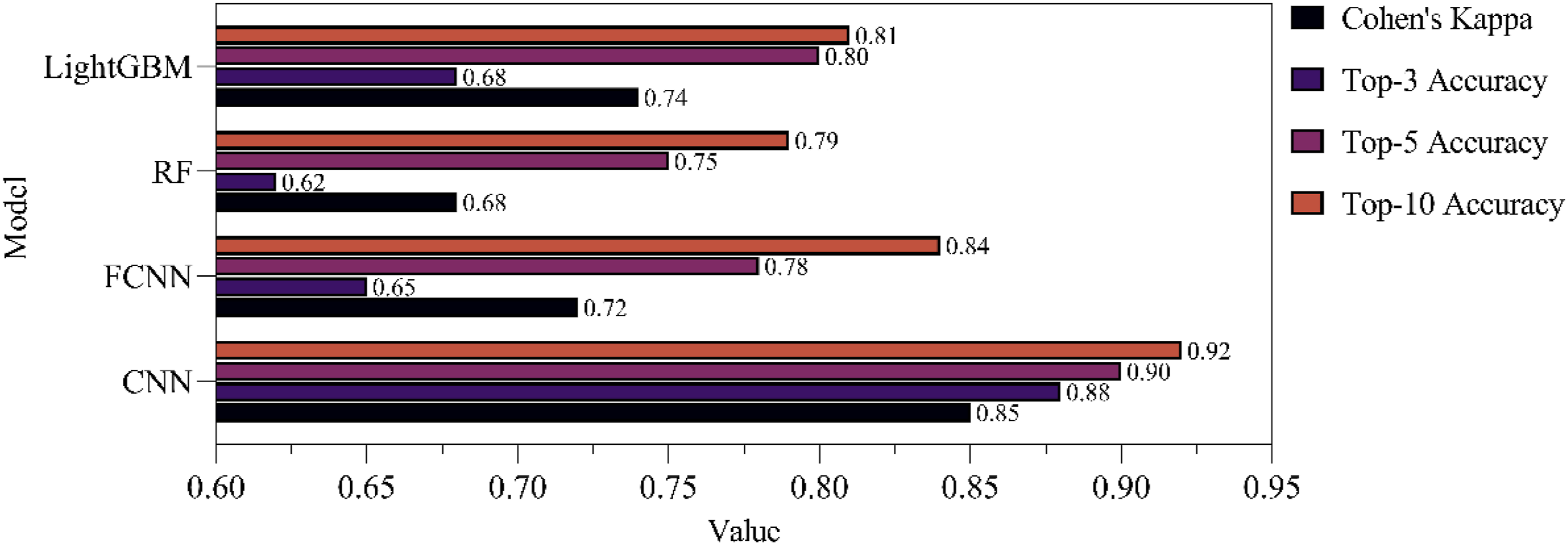

Figure 10 displays the performance comparison of the CNN model with feature stacking introduced in this article with FCNN, RF, and LightGBM in multi-label classification problems. The CNN model achieves 0.85 on Cohen’s Kappa evaluation indicator, which is significantly better than the other three models. It has better consistency in multi-label classification tasks. In addition, the model performs well in terms of Top-3, Top-5, and Top-10 accuracy, reaching 0.88, 0.90, and 0.92, respectively. In contrast, the performance of other models is relatively low. The CNN model can achieve more accurate recognition and classification in multi-label classification of musical instruments based on audio signals.

To further validate the performance of the model proposed in this article in real-time application scenarios, real-time recognition experiments are conducted to evaluate its performance in response time and computational resource consumption. The results of comparing the model in this article with FCNN, RF, and LightGBM are shown in Table 4.

Table 4.

Performance comparison of models in real-time recognition experiment.

Model	Average recognition time (seconds)	Average computational resource consumption (units)
Model in this article	0.05	1.2
FCNN	0.15	3.5
RF	0.20	4.0
LightGBM	0.18	3.8

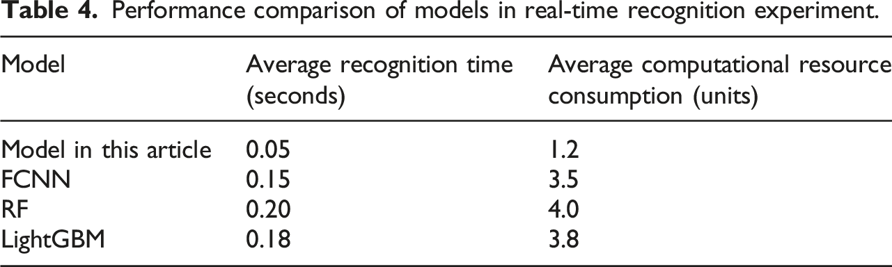
This article validates the performance of the model in real-world applications through real-time recognition experiments. The results show that the average recognition time of the model in this article is 0.05 seconds, consuming 1.2 units of computational resources, which is significantly better than FCNN, RF, and LightGBM models. The average recognition time of FCNN is 0.15 s, consuming 3.5 units. The RF execution time is 0.20 s, consuming 4.0 units. The running time of LightGBM is 0.18 s, and it consumes 3.8 units. These findings indicate that the model proposed in this article not only performs well in recognition speed, but also in computational resource efficiency, making it highly suitable for practical applications in real-time instrument recognition.

Conclusion

This article successfully utilizes CNN to achieve instrument recognition and analysis based on audio signals. Using FFT for spectral analysis and MFCC to describe spectral features, combined with time-domain and frequency-domain feature extraction methods, background noise and other interference factors can be effectively addressed in instrument performance. By training multiple CNN models and performing feature fusion and training in secondary CNN models, high instrument recognition accuracy is achieved, with an average precision of 0.90 and an overall recognition accuracy of 0.92. The evaluation results show that the method performs well on indicators such as AUC, MAE, and Cohen’s Kappa, with good stability and consistency. However, this article has also realized that there are still certain recognition errors in complex environments, and there is still room for improvement in the recognition of certain instruments. In future research, algorithms can continue to be optimized and more advanced deep learning techniques and data augmentation methods can be applied to improve the robustness and generalization ability of the model, further improving instrument recognition based on audio signals. In noisy public places, quiet recording studios, and outdoor environments, variations in instrument volume and background noise can significantly affect recognition performance. Future testing should include different background noise levels, volumes, and environmental conditions to ensure performance under various real-world conditions. This can help comprehensively understand the model’s stability and reliability in practical applications and provide support for future improvements.

Footnotes

Funding

The author received no financial support for the research, authorship, and/or publication of this article.

Declaration of Conflicting Interests

The author declared no potential conflicts of interest with respect to the research, authorship, and/or publication of this article.

References

Hendrik

Tuomas

, et al. Deep learning for audio signal processing. IEEE Journal of Selected Topics in Signal Processing 2019; 13(2): 206–219.

Siphocly

NNJ

El-Horbaty El-Sayed

Salem Abdel-Badeeh

. Top 10 artificial intelligence algorithms in computer music composition. International Journal of Computing and Digital Systems 2021; 10(01): 373–394.

Tang

Francisco

, et al. Deep cross-modal correlation learning for audio and lyrics in music retrieval. ACM Trans Multimed Comput Commun Appl 2019; 15(1): 1–16.

Gabriel

S-L

Juan-Carlos

G-H

Roberto

R-R

. Automatic Parkinson disease detection at early stages as a pre-diagnosis tool by using classifiers and a small set of vocal features. Biocybern Biomed Eng 2020; 40(1): 505–516.

Tan

Yong

Shi-Xiong

, et al. Audio-visual speech separation and dereverberation with a two-stage multimodal network. IEEE J Sel Top Signal Process 2020; 14(3): 542–553.

Fen

Liu

Yuejin

, et al. Feature extraction and classification of heart sound using 1D convolutional neural networks. EURASIP J Appl Signal Process 2019; 2019(1): 1–11.

Qinghe

Penghui

Yang

, et al. Spectrum interference-based two-level data augmentation method in deep learning for automatic modulation classification. Neural Comput Appl 2021; 33(13): 7723–7745.

Jessica

R-T

Cordova

EDM

. Analysis of speech separation methods based on deep learning. Res Comput Sci 2019; 148(9): 21–29.

Birajdar Gajanan

Patil Mukesh

. Speech/music classification using visual and spectral chromagram features. J Ambient Intell Humaniz Comput 2020; 11(1): 329–347.

10.

Xin

Zhang

. Music genre classification based on auditory image, spectral and acoustic features. Multimed Syst 2022; 28(3): 779–791.

11.

Anusha

Valiveti

Kumar

. Feature extraction algorithms to improve the speech emotion recognition rate. Int J Speech Technol 2020; 23(1): 45–55.

12.

Renato

Ricardo

Pedro

. Audio features for music emotion recognition: a survey. IEEE Trans Affect Comput 2020; 14(1): 68–88.

13.

Arun

Pandey

. Music instrument recognition using deep convolutional neural networks. Int J Inf Technol 2022; 14(3): 1659–1668.

14.

Prabavathy

Rathikarani

Dhanalakshmi

. Classification of musical instruments using SVM and KNN. Int J Innovative Technol Explor Eng 2020; 9(7): 1186–1190.

15.

Saranga Kingkor

Rahman

KAFU

Partha

. Deep neural network for musical instrument recognition using mfccs. Comput Sist 2021; 25(2): 351–360.

16.

Snigdha

Kavitha

Neginhal

, et al. Music genre classification using machine learning algorithms: a comparison. Int Res J Eng Technol 2019; 6(5): 851–858.

17.

Remi

Geoffroy

. An analysis of the effect of data augmentation methods: experiments for a musical genre classification task. Trans Int Soc Music Inf Retr 2019; 2(1): 97–110.

18.

Makarand

Amod

Parag

. Melodic pattern recognition in Indian classical music for Raga identification. Int J Inf Technol 2021; 13(1): 251–258.

19.

Rongfeng

Qin

. Audio recognition of Chinese traditional instruments based on machine learning. Cognitive Computation and Systems 2022; 4(2): 108–115.

20.

Kai

. Specifying the perceptual relevance of onset transients for musical instrument identification. J Acoust Soc Am 2019; 145(2): 1078–1087.

21.

Chai Xiu

Lee Choo

Lai

. Classifying musical instrument using spatiotemporal features with deep neural networks. Sensors & Transducers 2023; 263(4): 119–130.

22.

Sangeetha

Nalini

. Recognition of musical instrument using deep learning techniques. Int J Inf Retr Res (IJIRR) 2021; 11(4): 41–60.

23.

Tang

Chen

. Combining CNN and broad learning for music classification. IEICE Trans Info Syst 2020; 103(3): 695–701.

24.

Prabavathy

Rathikarani

Dhanalakshmi

. Classification of musical instruments sound using Pre-trained model with machine learning techniques. Asian Journal of Electrical Sciences 2020; 9(1): 45–48.

25.

Serhat

Serdar

Zekeriya

. Music emotion recognition using convolutional long short term memory deep neural networks. Eng Sci Technol Int J 2021; 24(3): 760–767.

26.

Jiangyan

Lin

Ashutosh

. An automatic instrument recognition approach based on deep convolutional neural network. Recent Advances in Electrical & Electronic Engineering (Formerly Recent Patents on Electrical & Electronic Engineering) 2021; 14(6): 660–670.

27.

Zhang

. Extraction and recognition of music melody features using a deep neural network. J vibroeng 2023; 25(4): 769–777.

28.

Lekshmi

Rajan

. Multiple predominant instruments recognition in polyphonic music using Spectro/Modgd-gram fusion. Circ Syst Signal Process 2023; 42(6): 3464–3484.

29.

Rajib

Choudhury

Dutta

, et al. Recognition of emotion in music based on deep convolutional neural network. Multimed Tool Appl 2020; 79(1): 765–783.

30.

Kim

Lee

Nam

. Comparison and analysis of SampleCNN architectures for audio classification. IEEE J Sel Top Signal Process 2019; 13(2): 285–297.

31.

Yagya Raj

Joonwhoan

. Deep learning-based late fusion of multimodal information for emotion classification of music video. Multimed Tool Appl 2021; 80(2): 2887–2905.

32.

Remzi

GUI

. Classification of instrument sounds with image classification algorithms. International Journal of 3D Printing Technologies and Digital Industry 2023; 7(3): 513–519.

33.

Joshi

Pareek

Ambatkar

. Comparative study of Mfcc and Mel spectrogram for Raga classification using CNN. Indian J Sci Technol 2023; 16(11): 816–822.

34.

Florian

Khaled

Gerhard

. Dynamic convolutional neural networks as efficient pre-trained audio models. In: IEEE/ACM transactions on audio, speech, and language processing, 24 October, 2023. DOI: 10.1109/TASLP.2024.3376984.

35.

Humphrey

Simon

Brian

. OpenMIC-2018: an open data-set for multiple instrument recognition. In: ISMIR, 1 september, 2018, pp. 438–444. DOI: 10.5281/zenodo.1432912.