Optimized wavelet transform based fault ranging of transmission line in substation

Abstract

To address the issue of insufficient positioning accuracy caused by faults in the transmission lines between substations, this study established a single-terminal travelling wave ranging model and proposed an optimized wavelet transform-based method for processing travelling wave signals. Using MATLAB as the simulation platform, we conducted simulations of single-terminal travelling wave ranging. The critical challenge in this method lies in accurately identifying the arrival time of the travelling wave signals. To address this, two different wavelet basis functions were selected to process the travelling wave signals, and their effectiveness in processing the same fault at different locations was compared and analyzed. The results show that the db4 wavelet better retains the original signal features. The error range for the Haar wavelet was 0.4289–0.6948 km, while for the db4 wavelet it was 0.0301–0.2960 km. Thus, the db4 wavelet provides more accurate ranging than the Haar wavelet.

Keywords

transmission line single-ended travelling wave ranging wavelet basis function optimized wavelet transform

Introduction

Transmission lines are core components of power systems, responsible for connecting power plants, substations, and users to ensure the stable transmission of electric energy.¹ As electricity demand increases, the power grid continues to expand, and line operation safety directly affects the reliability of the entire power system. Due to the long length and wide distribution of transmission lines—often affected by varying climatic and topographical conditions along their routes; the likelihood of faults is high, and fault patrols are challenging.² Therefore, fast and accurate fault point location plays a crucial role in ensuring timely repairs and maintaining power supply safety.^3,4

Traditional fault ranging methods are mainly classified into two categories: impedance and travelling wave methods.^5,6 The impedance method is based on the line parameter model and estimates the fault distance by calculating the amplitude-phase change of voltage and current before and after the fault, which has the advantage of simple implementation and lower cost. However, the method is susceptible to the interference of line parameter asymmetry, transition resistance, system oscillation and other factors, and the ranging accuracy is limited, which makes it difficult to meet the accuracy requirements of high-voltage/ultra-high-voltage lines. In contrast, the travelling wave fault ranging method uses the time difference between the propagation of the transient travelling wave signal generated by the fault between the fault point and the measurement point to locate the fault point, which has the significant advantages of clear principle, strong transition resistance, high accuracy, etc., and is especially suitable for long-distance transmission lines.⁷

The core of traveling-wave fault location lies in capturing and accurately identifying the arrival time of the initial wavefront generated by the fault at the measurement point (single-ended method) or comparing the time difference of the wavefront’s arrival at the two ends of the line (double-ended method).^8,9 The single-ended A-type travelling wave method is uniquely attractive for engineering applications due to its elimination of the need for a line-to-end synchronization device, its low cost, and its relative simplicity of implementation.¹⁰ The principle is based on the calculation of the fault distance based on the time difference between the initial voltage/current travelling wave of the fault detected at the measurement point and the arrival of its reflected wave at the point of fault.¹¹ However, the practical accuracy of the method is highly dependent on the precise detection and localization of the weak, high-frequency and often noise-drowned travelling waveheads. Therefore, signal processing techniques, especially time-frequency analysis tools, play an indispensable role here.

Wavelet transform, as a powerful time-frequency localization analysis tool, is particularly well-suited for processing non-stationary, transient traveling-wave signals due to its ability to reveal signal characteristics simultaneously in both the time and frequency domains and its multi-resolution analysis capability.^12–14 The wavelet transform provides a more accurate measurement of the time difference between the arrival of travelling waves at the detection points at each end of the line. Combined with the line length and wave propagation speed, these data help to calculate the fault location. This measurement method is not affected by factors such as transition resistance at the fault point or line structure and provides highly accurate ranging in a wide range of applications.¹⁵ Currently, multi-scale decomposition of travelling wave signals using wavelet transform to find the mode maxima in high-frequency details has become a mainstream method to locate the arrival moment of travelling waveheads.¹⁶ However, different wavelet functions have different roles in signal processing and relatively few studies have been conducted to compare and select wavelet functions. Therefore, in this study, different wavelet functions are selected for optimizing the wavelet transform.

This study employed single-terminal traveling-wave ranging technology to achieve fault location on transmission lines in substations. A transmission line simulation model was constructed on the MATLAB/Simulink platform to simulate traveling-wave propagation under faults at different locations. By systematically comparing the processing effects of different wavelet functions on fault signals, their performance differences in noise suppression, time-frequency focusing, and singularity detection were analyzed. Emphasis was placed on optimizing the identification accuracy of the wavefront transient time, thereby enhancing fault location accuracy.

Travelling wave fault ranging method

The travelling wave fault ranging method is a method for transmission line fault ranging based on travelling wave transmission theory.¹⁷ This paper describes the currently available methods of travelling wave localization, which can be categorized into four different methods, A, D, C, and E. To accurately locate type A faults, we calculated the product of the travelling wave’s round-trip time difference—generated by the fault—and the wave velocity between the measurement end and the fault point, enabling precise localization. The central point of the D-type technique is that it requires calculating the product of the time difference produced by the faulty travelling wave at each end and its speed, which enables the exact location of the fault point to be determined. Type C devices operate on the principle that, in the event of a fault, one end of the circuit is subjected to a high-frequency or DC pulse. This pulse is then used to localize the fault based on the difference in distance from the transmitting device to the fault location. E-type technology employs electric-wave single-ended control based on the reclosing principle. This study focuses on a technical approach for single-ended A-type travelling wave ranging.

Type A single-terminal ranging method

Single-ended A-type travelling wave ranging is a fault location method that uses line-mode transient travelling waves. In the event of a ground fault on the line, the acquisition device closest to the fault point receives the first travelling wave at time T₁. At the same time, a portion of the wave is reflected at the fault point and returns to the acquisition device, which receives this second travelling wave at time T₂. The distance between the acquisition device and the fault point is determined by calculating the time difference between these two moments. The principle of the single-ended A-type travelling wave ranging method is shown in Figure 1. The ranging calculation formula is shown in (1)

L_{B X} = \frac{(T_{2} - T_{1}) V}{2}

(1)

Figure 1.

Schematic diagram of single-end travelling wave fault ranging.

Here, B represents the first end of the branch line, which is also the measurement end; X is the fault point; L_BX is the distance from the fault point to B; T₁ is the time at which the first travelling wave head arrives at B; T₂ is the time at which the second travelling wave head arrives at B; and V is the propagation speed of the travelling wave.

The effectiveness of the single-ended A-type travelling wave ranging technique depends on the reflection of the travelling wave generated at the fault point after it reaches the B-end, as well as the time difference between the wave’s arrival and its reflection. The key to this method lies in accurately identifying the time of a sudden change in the travelling wave signal. The single-ended travelling wave method is widely used due to its simplicity and low cost. It is well suited for scenarios where extremely high accuracy is not required, although its precision can be affected by several factors.

Extraction of travelling wave signals

Within the framework of single-ended travelling wave-based fault location for transmission lines, the precise identification of the forward and backward travelling waves generated by a fault constitutes a critical step. To address this, a typical transmission line fault model was established using a simulation platform. Detailed records of three-phase voltages and currents captured at the monitoring point across multiple datasets were successfully acquired through the MATLAB workspace. Through meticulous analysis of the specific waveform characteristics exhibited by these voltages and currents under fault conditions, the voltage components corresponding to the backward travelling wave and the forward travelling wave were distinctly identified and separated. The methodology employed for extracting these travelling wave components is elaborated in detail in the following section.

(1) To accurately obtain the transient measurements u and i of the three-phase voltages and currents, we extracted the fault components from the three-phase voltages and currents during a period following the fault. We then calculated their differences from the corresponding pre-fault values over a similar time period before the fault.

(2) We derived the corresponding modal values u_m and i_m for the transient quantities u and i of the three-phase voltages and currents by means of Clark’s modulus conversion, the calculation of which is described in detail below

i_{m} = Q_{i} \times i

(2)

u_{m} = Q_{i} \times u

(3)

Q_{i} = \frac{1}{3} [\begin{array}{l} 2 & - 1 & - 1 \\ 0 & 1 & - 1 \\ 1 & 1 & 1 \end{array}]

(4)

where Q_i is the Clark transform matrix.

(3) The following details the accurate calculation of the voltage 1 mode in the forward travelling wave u_f1 and the reverse travelling wave u_r1 by performing the following specific steps

u_{f} 1 = \frac{1}{2} (u_{m} 1 + i_{m} 1 \times Z_{c m} 1)

(5)

u_{r} 1 = \frac{1}{2} (u_{m} 1 - i_{m} 1 \times Z_{c m} 1)

(6)

Z_{c m} 1 = \sqrt{L_{m} 1 / C_{m} 1}

(7)

In this context, u_m1 and i_m1 denote the first modal components of the matrices u_m and i_m, respectively, which are obtained by extracting the second row from each matrix. L_m1 and C_m1 represent the positive-sequence inductance and capacitance per kilometer of the transmission line, respectively.¹⁸

We implemented the above algorithmic simulation procedure using MATLAB as the programming tool and executed it directly within the software. Using this method, we were able to calculate the forward and reverse travelling wave components of the voltage’s first mode and generate the corresponding waveform graphs. Finally, the wavelet-transformed travelling wave signal was obtained using a program in MATLAB.

Optimized processing of travelling wave signals

Wavelet transform analysis

The wavelet transform is the decomposition of a signal into components with different frequencies and time scales. This is achieved using the wavelet function, which has both localization and multi-resolution properties. Unlike the traditional Fourier transform, the wavelet transform provides information in both the time and frequency domains, making it highly effective in analyzing non-stationary signals. The core idea behind wavelet transform is to construct a set of wavelet bases by scaling and translating a mother wavelet with localized time-frequency structure. The projections of a signal onto different wavelet bases reflect its local time-frequency characteristics. The wavelet transform relies primarily on two factors: the choice of wavelet basis function and the decomposition scale.¹⁹

Optimization of the wavelet transform

Optimizing the wavelet transform can be achieved in two ways. First, selecting appropriate wavelet basis functions tailored to the characteristics of the signal is crucial, as this choice significantly affects the performance of the transform. Common wavelet basis functions include Haar, db4, Symlet, and Coiflet. Selection depends on the signal’s frequency content and decomposition requirements. Second, adjusting the number of decomposition layers determines the frequency and time resolution of the wavelet transform. Increasing the number of layers improves frequency resolution but also raises computational complexity. The number of decomposition layers was selected according to the requirements of specific applications.

For applications such as travelling wave ranging, the time-frequency localization, energy concentration, and spectral properties of wavelets are usually considered. The db4 wavelet typically has better frequency localization properties than the Haar wavelet, tends to have a better energy concentration in the time domain than the Haar wavelet, and provides a richer spectral distribution. In summary, although Haar wavelets perform well in some simple signal processing problems, db4 wavelets are usually better for travelling wave ranging applications that require high signal accuracy and complexity, as they provide better frequency localization, energy concentration, and spectral properties.

Single-ended travelling wave ranging simulation platform construction

In this study, a MATLAB/Simulink-based travelling wave simulation system for single-ended transmission line faults was built, and its main architecture is presented in Figure 2. This platform includes a three-phase power supply, measurement units for three-phase voltages and currents, modules with faults in the three-phase circuits, and transmission lines with distributed parameters. The voltage of the three-phase power supply was set to 110 kV, while the frequency was set to 50 Hz. The application of three-phase V–I measurements is mainly to determine the actual state of the three-phase voltage as well as the current at detection point B. The measurement was carried out based on a three-phase voltage and current. A Three-Phase Fault is a configuration element for faulted lines that identifies short-circuit faults by selecting one or more of the phase A, B, or C fault options. The Ground Fault option is used to determine whether the short-circuit fault involves a ground connection. The fault transition time is set to 0.02 s. The Distributed Parameters Line represents a transmission line with distributed parameters. The total line length is set to 200 km, and the frequency is set to 50 Hz. The fault location can be adjusted by changing the position along the transmission line. Scope V and Scope I are used to observe the three-phase voltage and current waveforms at Point B, respectively. The sampling frequency is set to 5e-6 s and the simulation runtime is set to 0.06 s. The parameter settings for the simulated lines are listed in Table 1.

Figure 2.

Block diagram of fault travelling wave simulation platform of single-end transmission line.

Table 1.

Simulation line parameters.

Parameter type	Resistance/(Ω/km)	Inductance/(H/km)	Capacitance/(F/km)
Positive sequence	0.01273	0.9337e-3	12.74e-9
Zero sequence	0.38640	4.1264e-3	7.751e-9

Example analysis

After constructing the simulation platform, its functionality was verified through multiple simulation cases to ensure reliability. Given the broad scope of possible scenarios, we selected two representative fault cases: single-phase grounded short-circuit faults (phase B) and two-phase grounded short-circuit faults (phase AB and two-phase) as case studies). These cases were used to verify the accuracy of the simulation platform. Based on this, both types of faults were used for travelling wave fault ranging analysis.

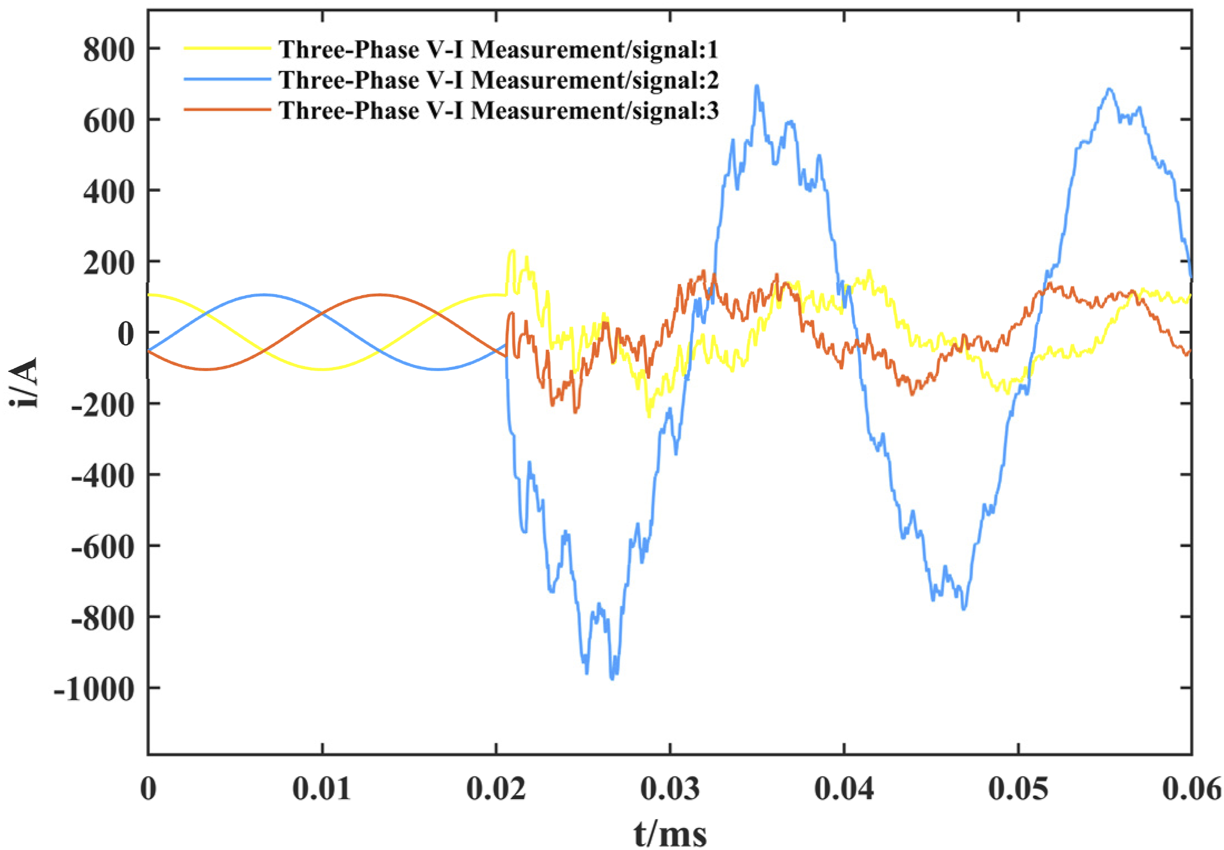
When the fault is defined as a short circuit to ground on phase B, a simple click on the simulation start button is required. Once the simulation process is complete, the oscilloscope is able to clearly display the three-phase voltage and current waveforms at the detection point internally, as illustrated in Figures 3 and 4.

Figure 3.

B three-phase voltage waveform under phase-phase short circuit.

Figure 4.

B Three-phase current waveform under phase-phase short circuit.

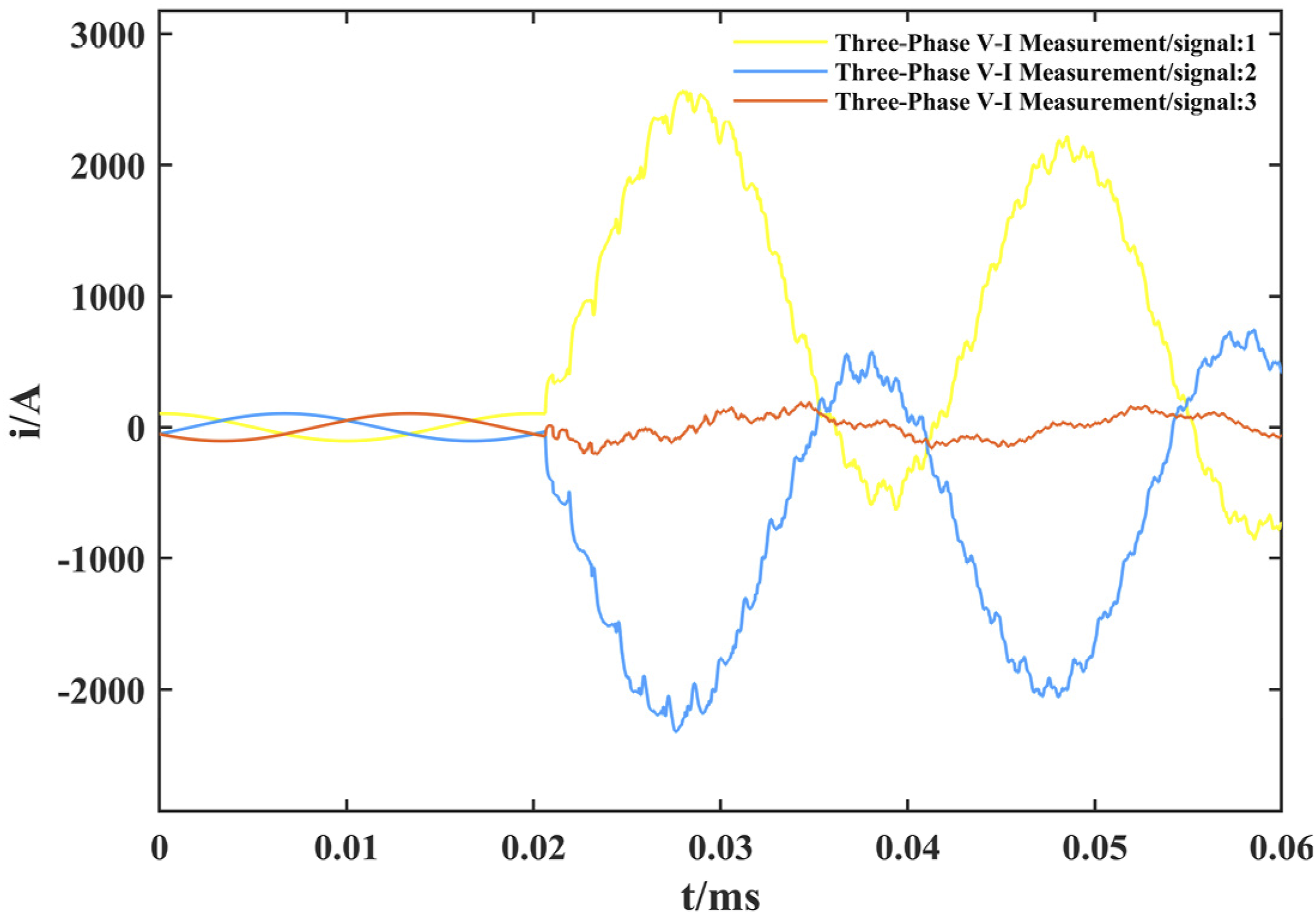
Then set the fault as a short-circuit to ground on both phases AB and simply click the simulation start button, once the simulation process is complete, the oscilloscope is able to clearly show the waveforms of the three-phase voltages and currents at the detection points internally, as shown in Figures 5 and 6.

Figure 5.

Three-phase voltage waveform under AB two-phase short circuit.

Figure 6.

Three-phase current waveform under AB two-phase short circuit.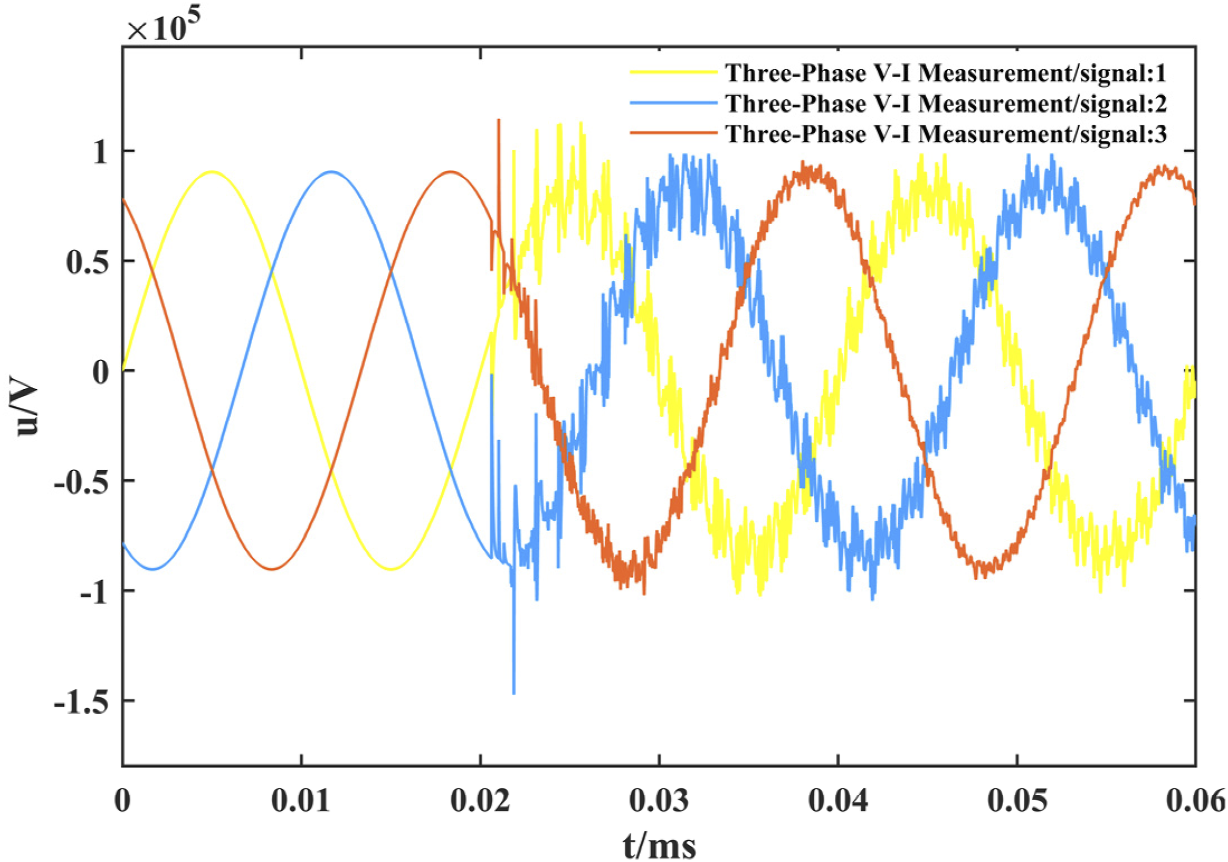

The behavior of the change rule of three-phase voltage and current waveforms under two different fault conditions was observed. The simulated waveforms obtained from the simulation were consistent with the expected characteristics of the line following a short circuit in phase A and a two-phase short-circuit fault in phases AB. Further confirming the accuracy of the simulation platform. In order to facilitate the observation of travelling wave signals, only the first 500 data points were considered in this study. First, the fault was set as an AB two-phase ground short circuit located 180 km from the measurement point. The simulation was run, and the three-phase voltage and current at the detection point were stored as arrays in MATLAB’s workspace. As shown in Figure 7, using a previously written MATLAB script, the relevant waveform information was efficiently extracted from the modeled three-phase voltage and current data.

Figure 7.

Voltage 1 mode forward and reverse travelling wave.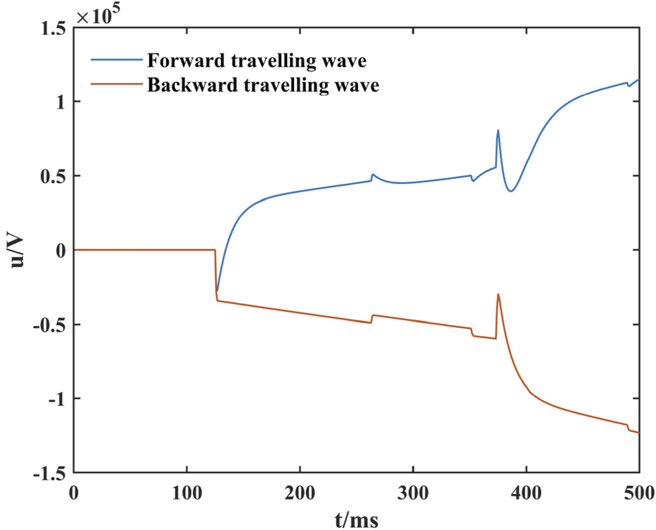

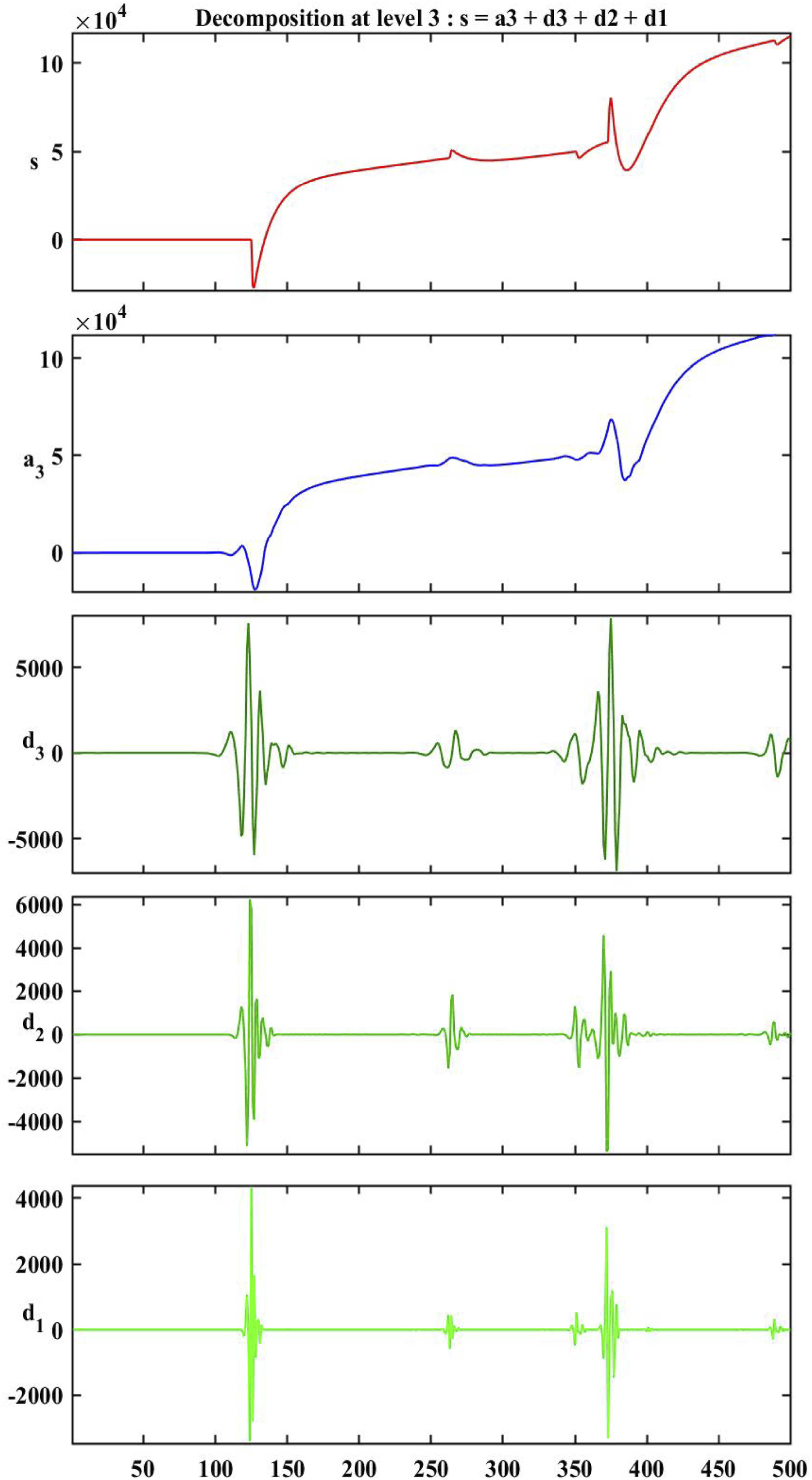
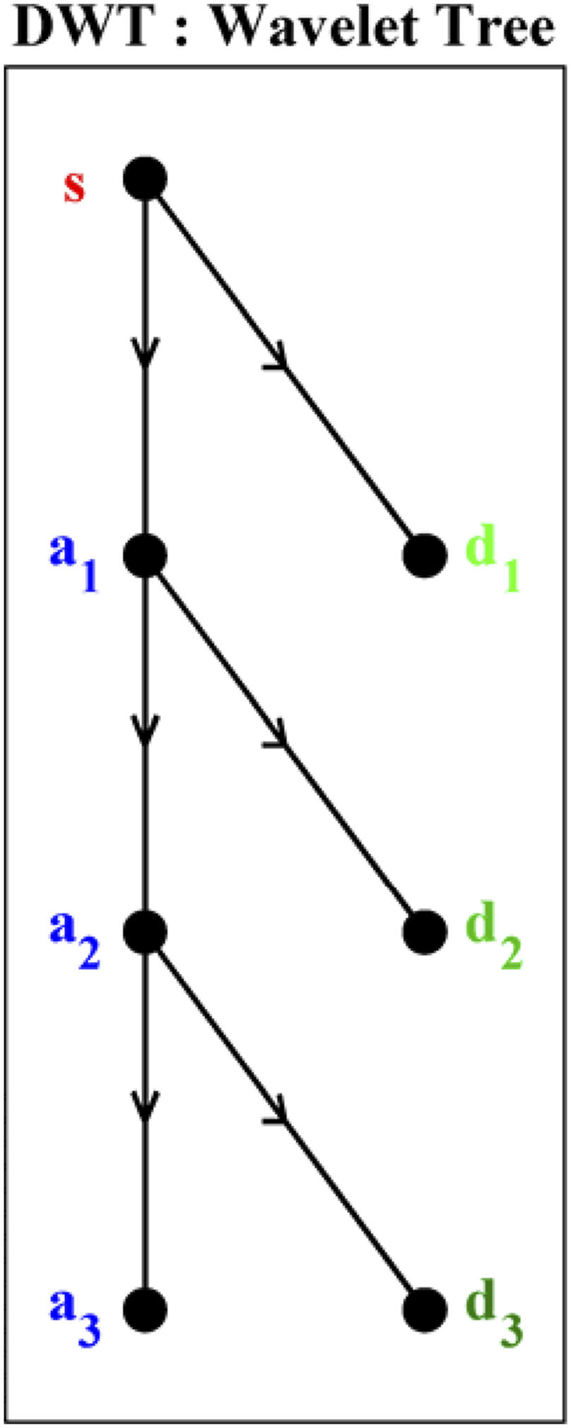
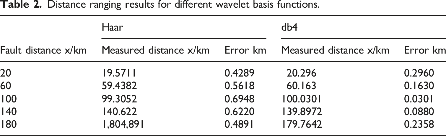
To precisely determine the arrival times of traveling wave signals, this study employed wavelet transform to analyze and process the captured signals. To evaluate the performance of different wavelet basis functions, two commonly used bases—the Haar wavelet and the db4 wavelet—were selected for transform optimization. Operating under the identical decomposition scale (fixed at three levels), traveling wave ranging calculations were performed using each basis function separately, and their ranging accuracies were compared. Signal processing was implemented utilizing the MATLAB toolbox. The decomposition results obtained with the two wavelet basis functions are presented in Figures 8 and 9, respectively. Analysis reveals that the amplitude of the approximation component (a3) is relatively large, while the amplitudes of the detail components (d3 to d1) decrease progressively. As the number of decomposition levels increases, the frequency components of the signal are partitioned more finely; the corresponding wavelet decomposition logic is illustrated in Figure 10. The arrival times of the initial wavefront and the subsequent reflected wavefront were precisely extracted from the processed signals. Based on a pre-programmed single-terminal traveling wave ranging method in MATLAB, the fault distance was calculated and the fault location was determined. To further validate the effectiveness of the method, the simulated fault location was varied multiple times, and multiple sets of traveling wave ranging experiments were conducted repeatedly. The results are presented in Table 2.

Figure 8.

Travelling wave signal after Haar treatment.

Figure 9.

Travelling wave signal after db 4 treatment.

Figure 10.

Wave wavelet decomposition logical relation.

Table 2.

Distance ranging results for different wavelet basis functions.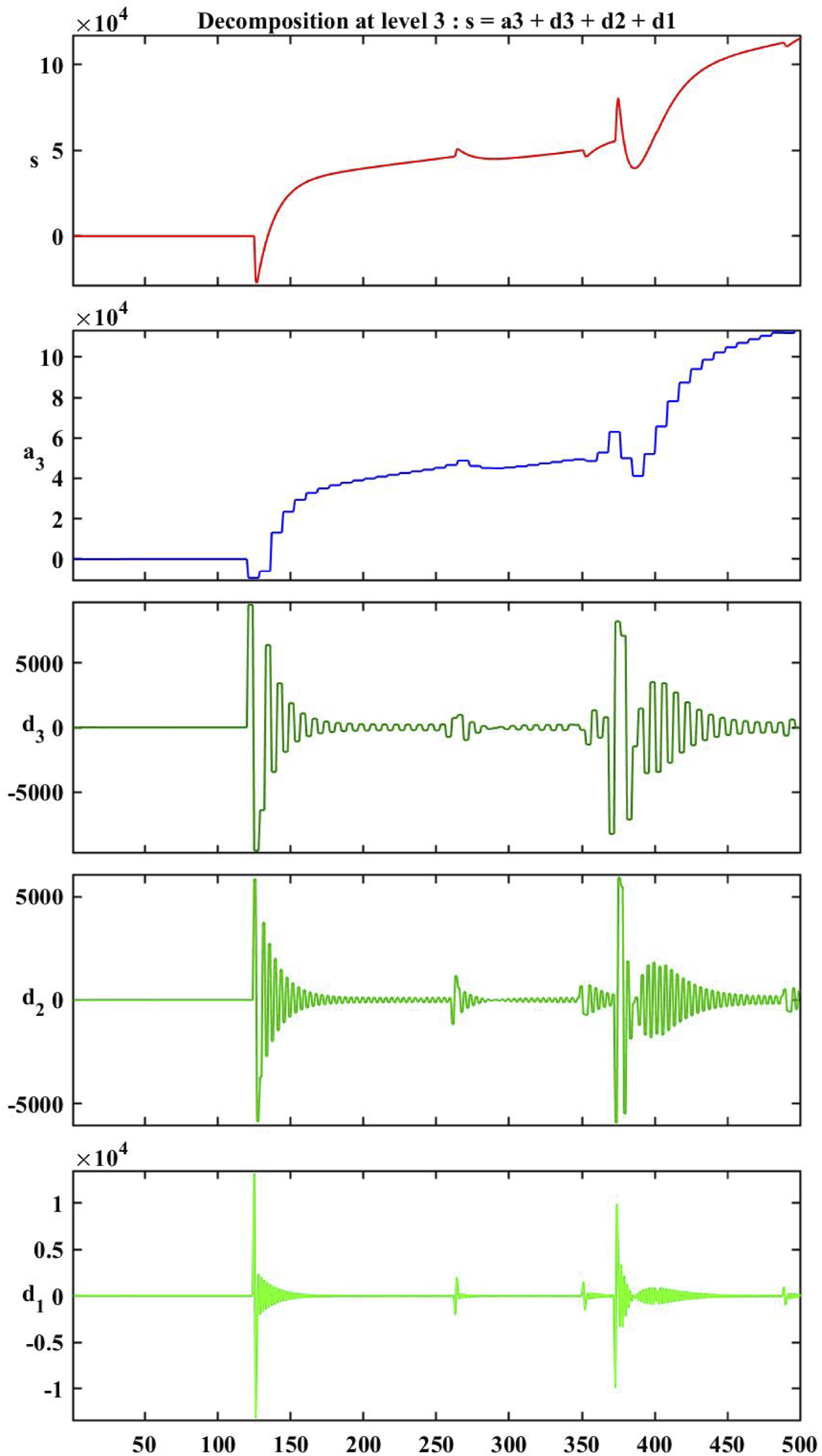

	Haar		db4
Fault distance x/km	Measured distance x/km	Error km	Measured distance x/km	Error km
20	19.5711	0.4289	20.296	0.2960
60	59.4382	0.5618	60.163	0.1630
100	99.3052	0.6948	100.0301	0.0301
140	140.622	0.6220	139.8972	0.0880
180	1,804,891	0.4891	179.7642	0.2358

Conclusion

In this study, an optimization of wavelet transforms was investigated for single-ended travelling wave fault ranging. MATLAB simulations and calculations were performed for five distinct fault locations under an AB two-phase grounded short-circuit condition. This approach facilitated the optimization of wavelet transforms utilizing various wavelet basis functions. Analysis and processing of the travelling wave signals enhanced noise immunity in the extracted signals and achieved precise extraction of wavefront arrival times.

(1) The travelling wave signal is susceptible to various types of interference in practical applications. However, using wavelet transform for travelling wave signal processing not only reduces noise interference but also accurately extracts the mutation time of the travelling wave signal, significantly improving the accuracy and reliability of distance measurement. (2) Overall, the db4 wavelet shows better characteristics in processing the travelling wave signals, particularly in preserving the original signal characteristics. Compared to the Haar wavelet, the db4 wavelet more effectively handles the mutation phenomena in travelling wave signals, making it more suitable and accurate for ranging applications. (3) Comparison of the ranging results for the same fault at different locations clearly shows that higher accuracy can be achieved using the db4 wavelet than with the Haar wavelet. Specifically, the Haar wavelet exhibited ranging errors between 0.4289 km and 0.6948 km, while the db4 wavelet achieved errors between 0.0301 km and 0.2960 km, indicating that the db4 wavelet provides more precise results in distance estimation.

Footnotes

Acknowledgements

The authors thank the support of the State Grid Shanxi Electric Power Company Technology Project (No. 52053024000Q). We would like to thank Editage () for English language editing.

ORCID iD

Rui Li

Funding

The author(s) disclosed receipt of the following financial support for the research, authorship, and/or publication of this article: This work was supported in part by the State Grid Shanxi Electric Power Company Technology Project (No. 52053024000Q).

Declaration of conflicting interests

The authors declared no potential conflicts of interest with respect to the research, authorship, and/or publication of this article.

References

Alcayde-García

Salmerón-Manzano

Montero

, et al. Power transmission lines: worldwide research trends. Energies 2022; 15(16): 5777.

Lin

Ouedraogo

, et al. A new fault location technique for three-terminal transmission grids using unsynchronized sampling. Int J Electr Power Energy Syst 2020; 123: 106229.

Wang

. Transmission line fault prediction and intelligent diagnosis method. Instrument Standardization & Metrology 2024; (2): 36–3848.

Pei

Liu

Yan

, et al. A method based on CNN and FFT-ELM for fault identification and location of transmission lines. J Electric Power Sci Tech 2024; 39(1): 164–170.

Yang

Deb

. Engineering optimisation by cuckoo search. Int J Math Model Numer Optim 2010; 1(4): 330–343.

Liu

Cheng

, et al. Fault location method for HV transmission line based on twoterminal synchronous response. Smart Power 2023; 51(12): 15–22.

Lee

Kim

Han

, et al. Fault area estimation using travelling wave for wide area protection. J Mod Power Syst Clean Energy 2016; 4(3): 478–486.

Lei

Hao

Dai

, et al. A review of fault location methods in HVDC transmission lines. Power System Protection and Control 2022; 50(11): 178–187.

Xao

Cheng

Cui

, et al. Study of comprehensive transmission line fault location method for smart substation. Power System Protection and Control 2016; 44(11): 40–45.

10.

Lei

Zhou

, et al. A single-terminal fault location algorithm in distribution network for eliminating the effect of the velocity of zero-mode travelling wave. Power System Protection and Control 2016; 44(23): 39–45.

11.

Rezaei

Gholipour

Parvaresh

. A single-ended traveling-wave-based fault location for a hybrid transmission line using detected arrival times and TW’ s polarity. Elec Power Syst Res 2022; 210: 108058.

12.

Ravesh

Ramezani

Ahmadi

, et al. A hybrid artificial neural network and wavelet packet transform approach for fault location in hybrid transmission lines. Elec Power Syst Res 2022; 204: 107721.

13.

Baroumand

Abbasi

Mahmoudi

. Integrative fault diagnostic analytics in transformer windings: leveraging logistic regression, discrete wavelet transform, and neural networks. Heliyon 2025; 11(4): e42872.

14.

García

Fresia

Mora-Merchán

, et al. A data-driven topology identification method for low-voltage distribution networks based on the wavelet transform. Elec Power Syst Res 2025; 243: 111517.

15.

Liu

Yao

, et al. Improved ultrasonic absolute stress measurement based on optimized wavelet transform and cross-correlation algorithm. Measurement 2025; 246: 116638.

16.

Wang

Zhao

Jin

. Multi-level and multi-scale cross attention network of wavelet packet transform for supersonic inlet unstart prediction. Expert Syst Appl 2025; 272: 126782.

17.

Liu

Xie

Kang

, et al. Parameter fitting-based traveling wave fault location method for multi-terminal DC grids. Int J Electr Power Energy Syst 2025; 164: 110412.

18.

Zhu

Fan

. Fault location scheme for a multi-terminal transmission line based on current travelling waves. Int J Electr Power Energy Syst 2013; 53: 367–374.

19.

Jamil

Kalam

Ansari

, et al. Generalized neural network and wavelet transform based approach for fault location estimation of a transmission line. Appl Soft Comput 2014; 19: 322–332.