Assessing the impact of financial asset structure on household consumption decisions in the digital age using neural networks

Abstract

The rapid digitization of finance has transformed household asset structures, introducing new financial instruments such as cryptocurrencies and digital investment platforms. However, the implications of this evolving asset composition on household consumption behavior remain underexplored. Traditional models often fall short in capturing the temporal and nonlinear dynamics of such relationships. Research aims to assess the impact of financial asset structures, including both traditional and digital assets, on household consumption decisions by leveraging advanced neural network architectures. The dataset comprises household-level financial and consumption data drawn from finance surveys, enriched with detailed metrics on digital asset ownership and usage. Key variables include household income, traditional and digital asset composition, demographic attributes, and monthly expenditure patterns. Data pre-processing involved handling missing values and outliers, followed by Z-score standardization to ensure normalization. A stacked Long Short-Term Memory (SLSTM) network was employed to model time-series consumption trends and capture underlying temporal dependencies. The Enriched Satin Bowerbird (ESB) algorithm was used to enhance training efficiency and convergence. The Enriched Satin Bowerbird mutated Stacked LSTM (ESB-SLSTM) model effectively identified complex nonlinear interactions and temporal patterns between asset structures and consumption behavior. Implemented using Python, the proposed ESB-SLTSM model accurately analyzes household consumption based on financial asset structures. It achieves over 93% in F1-score, accuracy, recall, and precision, ensuring robust and insightful behavioral predictions. Results indicate that households with significant digital asset holdings display more dynamic and sensitive consumption responses, particularly in response to market fluctuations. The model achieved superior predictive performance compared to baseline econometric models. These findings offer valuable insights for policymakers and financial planners aiming to promote stable consumption and responsible digital asset integration.

Keywords

finance asset structure digital age household consumption Enriched Satin Bowerbird mutated Stacked LSTM (ESB-SLSTM)

Introduction

Household consumption is a major part of any economy, which captures the goods and services consumed by individuals or families, relating to their survival and general well-being.¹ It encompasses a wide array of items, including food, clothing, housing, education, health care, recreational activities, and electronics or technology. In short, it captures the quality of life and lifestyle choices of the people in a society.² Therefore, household spend is the primary source of economic growth, influencing the market demand in the economy and influencing government decisions on taxation, subsidies, and welfare programs.³

The basic elements of household consumption are driven by many interrelated factors. The most fundamental element is income.⁴ In other words, the degree to which a household earns money through paychecks, business profits, pensions, or any other form of income directly relates to how much money it can spend. Along with income are the effects of expectations, saving time, the levels of interest rates, levels of inflation, family size and age, and cultural preferences on consumption decisions.⁵ Households attempt to balance spending to directly satisfy present consumption and save for future consumption. Households are positioned by the economy. In uncertain and job-insecure environments, households save more and consume less. In contrast, when the economy is stable and income levels are rising, consumption often increases.⁶

Financial asset composition refers to the method households organize and hold a variety of financial assets, from savings accounts, stocks, bonds, mutual funds, retirement fund vehicles, real estate, and digital currencies, to most recently, different fintech and digital investment platforms.⁷ In earlier decades, households primarily invested in physical assets, including gold, land, or bank savings. Today, with the increased availability of digital finance, households have access to a wide range of financial instruments.⁸ These include both traditional financial assets and newer digital ones such as cryptocurrencies, peer-to-peer lending, digital wallets, and mobile-based investment applications.⁹ This is shaping new financial behaviors impacting how families plan for the future, understand risk, and determine allocation of many forms of consumption and savings.¹⁰ The dynamics between a household’s financial asset structure and its consumption choices are increasingly relevant in the digital era.¹¹ The variations in digital platforms make it difficult to establish standardized measurements for financial asset use for households. Household preferences and socio-cultural aspects are challenging to measure and quantify. A lack of detailed financial records and privacy considerations also limits measurement.

This research aims to discover the impact of digital and traditional financial assets on household consumption in the digital age by employing an ESB-Stacked LSTM model to model nonlinearities in the patterns and time dependencies in financial data. The key contributions are as follows.

(1) Advancement of the ESB-SLSTM Framework: The ESB-SLSTM pre-trained model was introduced to evaluate the nonlinear effects of financial asset structures on household consumption decisions.

(2) Incorporation of Digital and Traditional Asset Structures: Both traditional and digital assets, cryptocurrencies, were integrated for a more comprehensive financial behavior analysis.

(3) Integration of Demographic and Financial Metrics: The model considers the relationship between household income, demographics, and asset types to improve predictions of consumption.

(4) Evaluation for Baseline Econometric Models: Displays increased effectiveness and robustness of the proposed ESB-SLSTM compared to standard methods.

Related works

This section reviews the existing literature on household consumption behavior, encompassing traditional economic models and more recent studies that explore the role of digital financial assets.

Utilizing data from the CHFS (2015–2019), Ma et al.¹² investigated the impact of digital financial usage on household consumption upgrading. Their research demonstrated that digital financial services optimize financial asset allocation across four areas: diversification of financial investment portfolios, participation in risky markets, augmentation of risky asset allocation, and the stimulation of improved consumption patterns. Shang et al.¹³ created an R-DB-LM-NN architecture and training algorithm to precisely forecast the closing price of cryptocurrencies. Their proposed method fared better than both deep learning (DL) and conventional machine learning (ML) techniques in terms of prediction performance. Experimental results indicated that the suggested architecture outperforms both DL and CNN models in prediction tasks. Liu¹⁴ examined the influence of AI development on the distribution of household financial assets using data from the 2019 CHFS and a Tobit model. The study observed that households allocate a larger percentage of their financial assets when AI development is higher, a finding confirmed as significant through robustness tests employing Probit and other models.

To predict Iran’s energy needs, Ahmadi et al.¹⁵ investigated intelligent forecasting techniques, including artificial neural networks (ANNs). By employing a deep neural network (DNN) with fuzzy wavelets to forecast energy consumption in several cities from 2010 to 2021, they achieved high-performance prediction at a reduced complexity level. For fraud detection, Huang et al.¹⁶ developed a framework employing a hybrid neural network with a clustering-based undersampling technique (HNN-CUHIT) to increase reliability. This framework learns user and transaction aspects to reveal personal background and economic conditions, outperforming other ML models with an F1-score of 0.0416 in handling imbalanced class solutions. Wu et al.¹⁷ investigated risk assessment techniques for agricultural Supply Chain Finance (SCF) to lower credit risks. They modified the weights and thresholds of a backpropagation neural network (BPNN) using a Genetic Algorithm (GA) and selected indicators with Principal Component Analysis (PCA). This GA-BPNN method streamlines the indicator selection procedure and accelerates the BPNN’s convergence rate, offering a viable approach for financial credit risk evaluation.

To reduce inherent noise in Bitcoin’s time-series data, Tripathi and Sharma¹⁸ suggested a trustworthy forecasting framework to explore the prediction capabilities of various indicators. Their approach employed deep neural networks, Hampel and Savitzky-Golay filters, and a three-step hybrid feature selection process for short-term price prediction. Chen and Long¹⁹ examined the application of AI algorithms to forecast financial hazards in Chinese e-commerce businesses. They used Long Short-Term Memory (LSTM) as a fitness function, employed factor analysis to lower overfitting risk, and optimized learning rates and hidden layer neurons through a Particle Swarm Optimization (PSO) algorithm. The resulting model achieved the lowest MSE, MAE, and MAPE values, enabling effective risk management and organizational sustainability.

Due to the absence of spatial local association in tabular data, DL techniques like convolutional neural networks (CNNs) were seldom used in credit assessment. To address this, Qian et al.²⁰ proposed a new end-to-end Soft Reordering 1D-CNN (SR-1D-CNN) that adaptively rearranges tabular data for CNN learning. Experimental results demonstrated that this method enhances CNN’s categorization effect for tabular data, outperforming other benchmark methods. Aydin et al.²¹ created a model for estimating and categorizing financial failures across various industries using ANN and decision trees (DTs). The model aimed to compare non-bankrupt rates and identify major factors influencing sector-level financial failures, accurately categorizing 240 listed enterprises on the BIST exchange. For the precious metals market, Mousapour Mamoudan et al.²² attempted to create new techniques for detecting false signals in technical analysis indicators. They suggested hybrid metaheuristic algorithms combining a Bidirectional Gated Recurrent Unit with a CNN, using the Firefly algorithm for hyperparameter optimization and the Moth-Flame Optimization (MFO) technique for feature selection. These metaheuristics may aid investor decision-making in financial and precious metals markets.

Dube et al.²³ developed and tested financial distress prediction models using ANN for firms listed on the Johannesburg Stock Exchange. The models achieved classification accuracies of 81.03% and 96.6%, successfully forecasting financial trouble up to 5 years in advance. Di Lorenzo et al.²⁴ employed a neural network approach to handle risk in Reverse Mortgage contracts. They utilized NN to effectively estimate nonlinear functions for calculating Conditional Value at Risk, ensuring accurate assessments of potential losses and portfolio solvency compared to traditional Value at Risk methods. Konak et al.²⁵ aimed to determine the factors influencing dividend distribution rates and create a framework for future projections. They employed a feed forward backpropagation ANN (FFBP-ANN) model with 26 input variables and created a hybrid model to optimize feature and parameter selection. Their experimental findings indicated that only five factors were required to predict the dividend distribution ratio accurately. Using an ANN technique, Magazzino et al.²⁶ examined the relationship between agricultural productivity, output, and credit availability from 2000 to 2012. Their study suggested an additive impact among these factors, with loan availability being more significant in OECD nations and less so in countries with lower economic development. The findings confirmed that access to credit majorly impacts productivity in both industrialized and emerging nations.

Prior research has demonstrated the efficacy of AI and DL techniques in enhancing financial forecasting and modeling household asset allocation. Nonetheless, limitations remain with regard to accurately representing the complex, nonlinear, and temporal relationships between evolving digital asset structures and household consumption patterns.

(1) Shang et al.¹³ presented an R-DB-LM-NN for predicting cryptocurrency closing prices. While it showed predictive durability, it only offered marginal improvements over traditional models. Furthermore, its application is confined to cryptocurrency markets, and it provides no generalizable framework for predicting broader household financial behaviors related to digital or traditional assets.

(2) Liu¹⁴ used a Tobit model on survey data to investigate the impact of AI development on household financial asset allocation. Although it found significant correlations, the employed econometric models are static and fail to account for the time-series complexity and nonlinear relationships that affect consumption.

To overcome these limitations, this research proposes the ESB-SLSTM model. This hybrid method combines the sequence learning capability of SLSTM to model time-dependent consumption trends with an ESB algorithm to achieve optimal convergence and parameter tuning. By modeling the effects of both traditional and digital assets through a temporally aware deep learning framework, the proposed model aims to achieve improved predictive precision, enhance the stability of the learning process, and yield deeper insights into modern financial decision-making behaviors.

Methodology

The methodology section describes the method used to assess how financial asset structures impact household consumption behavior. The initial step is to collect a dataset that consists of household income, types of assets, demographic information, and monthly expenses. The collected datasets are fed into data pre-processing steps, including handling missing values, outliers, and Z-score standardization to establish consistency and representativeness. To develop a model for time-based consumption patterns, an SLSTM network is used to capture sequential dependency. The SLSTM can improve its speed and quality of convergence by using the ESB algorithm to develop the ESB-SLSTM. The overall process for financial asset structure on household consumption is shown in Figure 1.

Figure 1.

Overall process for financial asset structure on household consumption.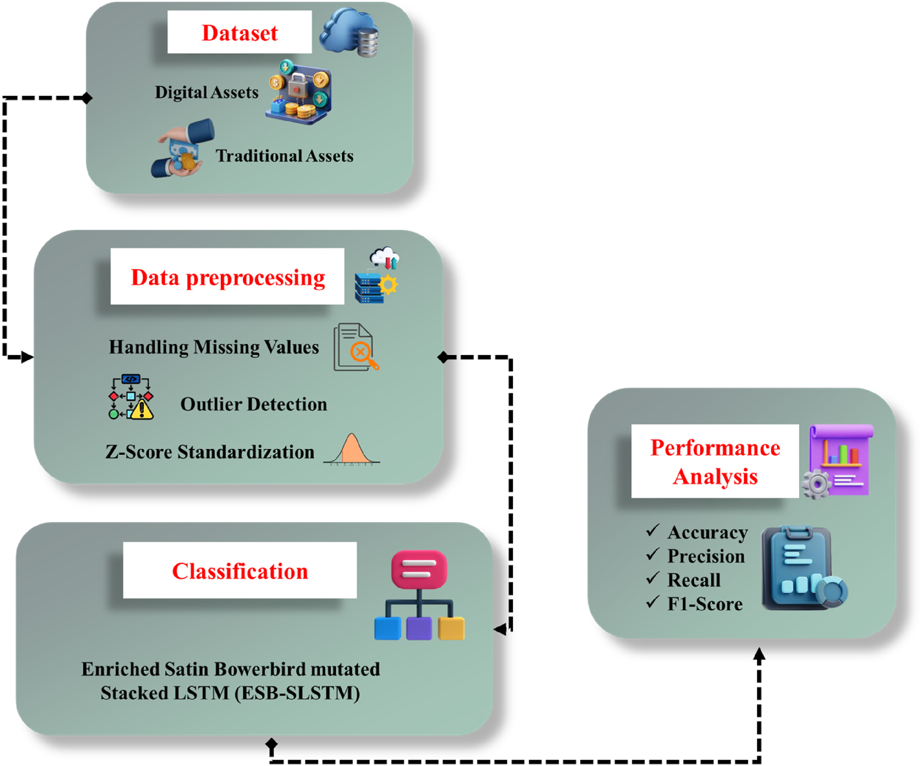

Dataset

The dataset utilized in this study is sourced from the publicly available China Household Finance Survey (CHFS). The CHFS provides comprehensive household-level data across multiple provinces in China, including detailed information on household demographics, income, financial asset holdings (both traditional and digital), expenditure patterns, employment status, and other socio-economic variables.

For the purpose of this research, the dataset was separated into two main files: one capturing digital asset ownership (cryptocurrencies, digital wallets, online stock investments, etc.) and the other detailing traditional financial assets (bank savings, bonds, real estate, insurance, gold, etc.). Each record corresponds to a household at a specific survey date, enabling the construction of temporal asset and expenditure trajectories. To mitigate potential biases, the dataset was carefully examined for representativeness, and sampling weights provided by the survey were considered in the analysis. While the data is China-specific, it encompasses a broad demographic spectrum, making it a valuable source for understanding household financial behaviors within this context.

Source: https://www.kaggle.com/datasets/programmer3/household-asset-impact-on-consumption.

Data pre-processing

The data pre-processing stage consisted of three steps: missing values, outlier detection, and Z-score standardization. After identifying missing data from the interpretive data, the missing data were either deleted or imputed with average or median values that were relevant. Following the handling of the missing data, outliers were determined using IQR and Z-score techniques. Data were then either capped or corrected. Once the outliers were processed, Z-score standardization was applied to normalize the scale of the features in the data. The above steps ensured data quality for the use of neural networks.

Handling missing values

Handling missing values was the first step in data processing to accurately capture the relationship between the structure of financial assets and household consumption behavior. Variables were checked for missing entries, and records were removed based on too much missing data to affect learning patterns. For features with only limited number of missing variables mean or median imputation can be performed, depending on the variable’s distribution and importance. This process ensures complete and clean data to allow the neural network model to learn with a high-quality dataset, without damaging predictive performance.

Outlier detection

Outlier detection was required to enhance the quality of the data to accurately simulate household consumption behavior. Specifically, the methods used to identify abnormal values included IQR and Z-score. Both methods detected values that deviated significantly from the expected. Their outliers were either capped or adjusted. These outliers were removed to avoid skew during modeling. Removing outliers provided the greatest opportunity for the neural network to effectively identify genuine trends in financial behaviors.

Z-score standardization

Z-score standardization was used in data pre-processing to accomplish the modeling of household consumption behavior influenced by a variety of financial assets. This technique can ensure that all numerical features are considered equally during training by putting them on the same scale. This technique is especially valuable for neural networks where different and inconsistent data ranges can slow learning and convergence. Predictive accuracy, learning speed, and model stability were all improved by standardizing the data. The z-score standardization equation (1) is described as follows:

Z = \frac{Y - μ}{σ}

(1)

The standardized score $Z$ is derived by subtracting the mean $μ$ of the feature from the original data point $Y$ , and then by dividing by the standard deviation $σ$ of that feature. It transforms the data such that, it is centered at zero and scaled according to its variability. After this transformation, the data will have a mean of 0 and a standard deviation of 1. This standardization step will allow the neural network to use the input data more effectively and avoid bias toward features with larger numeric scales.

Then, the pre-processed data are fed into the proposed ESB-SLSTM model to effectively identify complex nonlinear interactions and temporal patterns between asset structures and household consumption behavior.

Enriched Satin Bowerbird mutated Stacked LSTM (ESB-SLSTM)

The ESB-SLSTM was developed to model the dynamic and nonlinear relationship between structures of financial assets and household consumption. The hybrid approach harnesses the high-level temporal learning ability of Stacked LSTM with the optimization effectiveness of ESB to facilitate training convergence and improve prediction accuracy in inherently complex financial datasets.

The ESB algorithm draws inspiration from the foraging behavior of satin bowerbirds, which are known for their complex and adaptive foraging strategies. In the context of neural network optimization, the ESB employs two key mechanisms to enhance convergence: chaotic initialization and Cauchy mutation. Chaotic initialization utilizes a logistic chaotic map to generate diverse and unpredictable initial solution populations, thereby increasing the exploration capacity of the algorithm and reducing the risk of premature convergence to local minima. Specifically, the logistic map produces a sequence with sensitive dependence on initial conditions, ensuring a wide coverage of the solution space.

Following initialization, the Cauchy mutation introduces large, unpredictable perturbations to candidate solutions, enabling the algorithm to escape local optima by exploring regions of the search space that are otherwise difficult to access with traditional mutation strategies. The Cauchy distribution’s heavy tails facilitate occasional significant jumps, promoting diversity and robustness during optimization. Collectively, these mechanisms allow the ESB to effectively navigate complex, nonlinear error landscapes in neural network training, thus improving convergence speed and predictive accuracy. The algorithm ensures that the network’s final parameters can learn the nonlinear dependencies between asset composition and spending patterns. Logistic chaos will support initial population diversity and speed up optimization. The initialization population of an ESB is given by equation (2):

p o p (j) . P o s i t i o n = Y (j, :) * (V a r M a x - V a r M i n) + V a r M i n

(2)

This Equation ensures diverse solution candidates using chaotic sequences, improving learning coverage in financial datasets.

SLSTM captures sequential consumption patterns by stacking multiple LSTM layers, which allows us to map temporal dependence more effectively. It resolves the problem of short-term memory loss by utilizing gated memory cells. The hidden state $T_{s}$ is calculated as follows, equation (3):

T_{s} = H_{p} ⨀ \tanh (θ_{s})

(3)

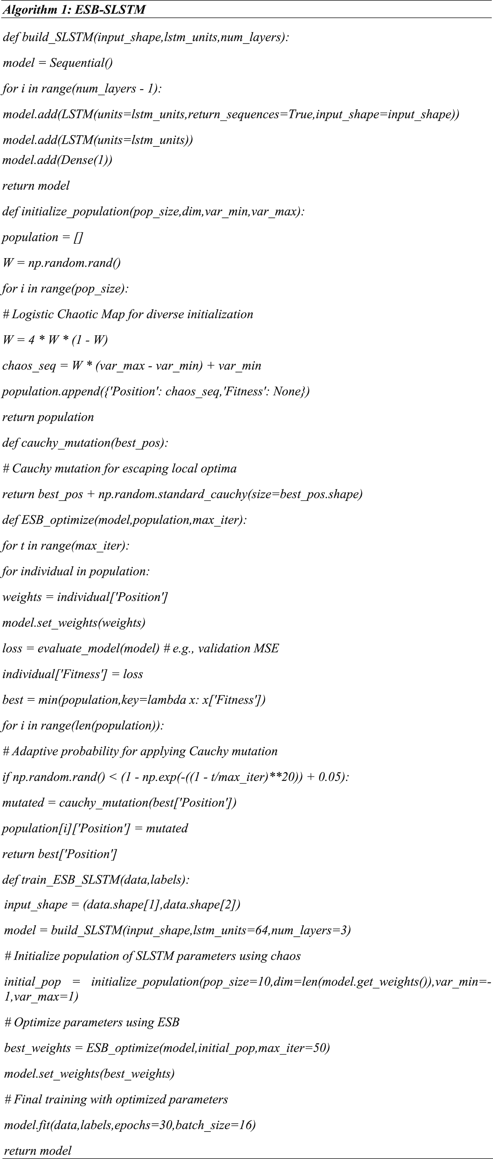
This equation outputs the current memory by modulating internal state $θ$ , with output gate $H_{p}$ reflecting relevant consumption signals over time.

The proposed ESB-SLSTM hybrid method is a model of the evolving financial asset structure solution and household consumption as an optimal nonlinear and time-dependent relationship. The ESB global optimization was relatively solved using SLSTM’s deep-temporal modeling. The model provided excellent convergence and improvement in the prediction. Algorithm 1 shows the pseudocode for ESB-SLSTM.

Stacked LSTM (SLSTM)

An SLSTM is a deep learning architecture that can handle sequential data by learning long-term dependencies. It seeks to learn a temporally complex pattern contained in a time-series dataset, like time-based changes in household consumption. The model learns the sequence behavior at each layer by stacking multiple LSTM layers, therefore, it has a richer representation and better predictive performance in uncertain environments.

LSTM is a recurrent neural network that can learn and predict order dependence in sequence identification tasks. Feedback connections allow for the efficient processing of an entire data series. Short-term memory loss is avoided by using LSTM, which is made up of cells and gates that control the flow of information. An LSTM layer is a group of memory blocks that are connected recurrently. Digital processors’ differentiable memory chips are comparable to these units. Each of them contains input, output, and forget gates, together with one or more memory cells connected in a loop. For the memory cells, these three multiplicative units continuously simulate writing, reading, and resetting. The subsequent equations (4)–(6) are used to determine the input, output, and forget gates:

H_{j} = σ (z_{s} X_{z j} + T_{s - 1} X_{t j} + β_{j})

(4)

H_{e} = σ (z_{s} X_{z e} + T_{s - 1} X_{t e} + β_{e})

(5)

H_{p} = σ (z_{s} X_{z p} + T_{s - 1} X_{t p} + β_{p})

(6)

Where

z_{s}

denotes the current input,

T_{s - 1}

is the previous concealed state, and

β_{j}, β_{e}, and β_{p}

are the biases for each gate.

X_{z j}, X_{z e}, X_{z p}, X_{t j}, X_{t e}, {and X}_{t p}

are the weight metrics;

H_{j}

H_{e},

and

H_{p}

represent forget, input, and output gates. The symbol

σ

refers to the sigmoid activation function. Equation (7) is used to calculate the input node memory cell

{\tilde{θ}}_{s}

{\tilde{θ}}_{s} = \tanh (z_{s} x_{z d} + T_{s - 1} x_{s c} + β_{d})

(7)

Where

\tanh

is the hyperbolic tangent function,

x_{s c} and x_{z d}

are the weight matrices for the candidate state. Equation (8) is used to calculate the internal state of the memory cell

θ_{s}

. The symbol

⨀

indicates element-wise multiplication.

θ_{s} = H_{e} ⨀ θ_{s - 1} + H_{j} ⨀ {\tilde{θ}}_{s}

(8)

Equation (9) uses the activation function to calculate the hidden state $T_{s}$ .

T_{s} = H_{p} ⨀ \tanh (θ_{s})

(9)

The time step in this case is $s$ , and the input is $z_{s}$ . Unlike the typical LSTM model, which only has one hidden layer, the stacked LSTM model has multiple hidden layers. The model’s ability to adjust nonlinear processes using raw data and attain faster convergence is advantageous, while the model’s parameters are dispersed across its space without requiring more memory. In Figure 2, the architecture of the stacked LSTM model is displayed.

Figure 2.

Architecture for SLSTM.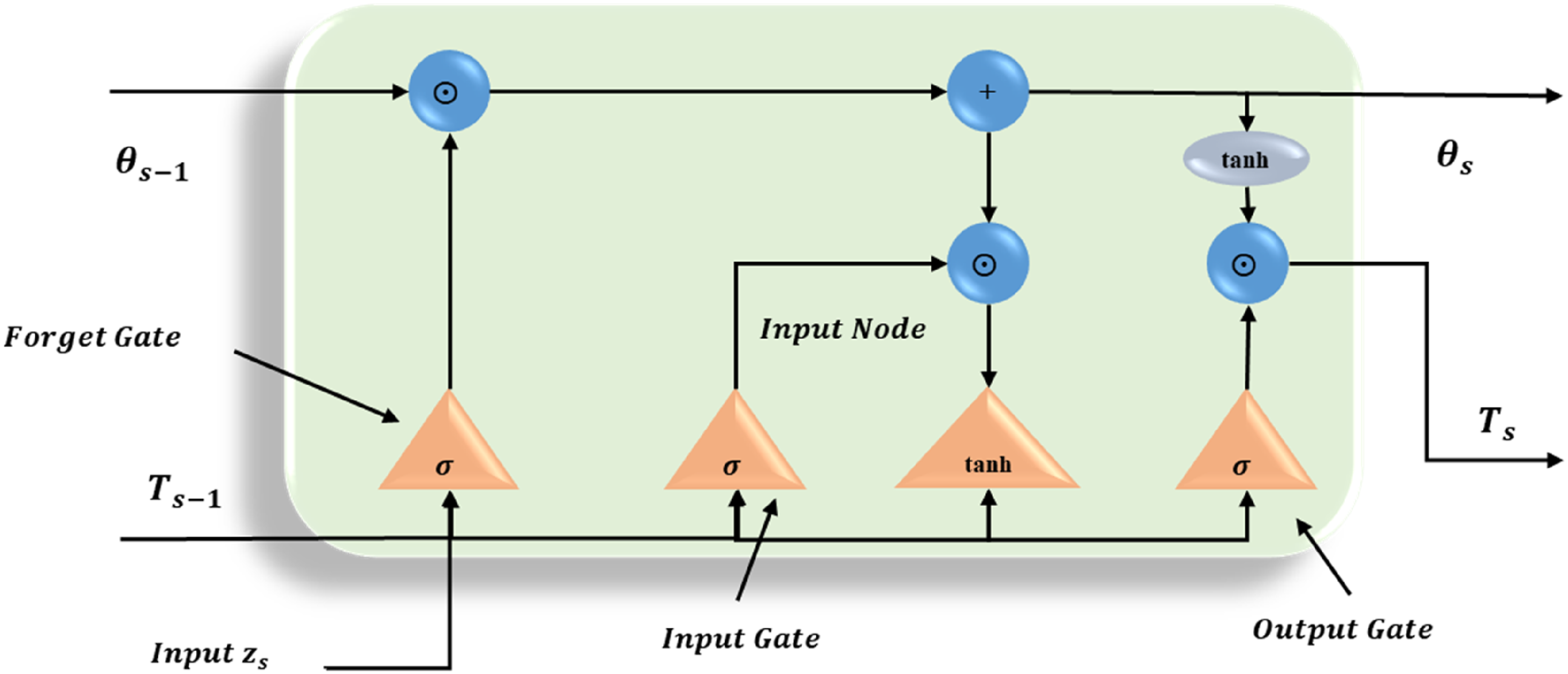

Enriched Satin Bowerbird (ESB)

The ESB algorithm aims to improve the training efficiency and convergence of the model in terms of understanding household consumption. ESB guarantees that network parameters can accurately learn the nonlinear and temporal relationships that exist in relations for financial asset structures and spending behavior. The ESB algorithm introduces adaptive exploration strategies, which stem from the foraging behavior seen in satin bowerbirds, to ensure that the model can escape from local optima, which ultimately produced a better-performing predictive model in complex financial data environments.

Initialization of logistic chaos

Utilizing logistic chaos initialization to efficiently optimize the ESB-SLSTM model for financial behavior modeling maximizes population diversity and speeds convergence, limiting premature local minima. This initialization allows sufficient exploration of the underlying solution subspace to learn effectively the nonlinear relations for asset-consumption.

A better initialization technique will significantly speed up the intelligent optimization algorithm’s convergence speed, even though the initial population of the algorithm uses a random initialization mode for each natural law. This depends on the engineering application’s goals and convergence speed requirements. Additionally, the ESB initializes the population using random values. As a result, a logistic chaotic map can increase the initial population’s diversity, which will improve the initial population and, eventually, the algorithm’s optimization accuracy and convergence time. Equation (10) illustrates the logistic chaotic map calculating method:

W_{j + 1} = μ W_{j} * (1 - W_{j})

(10)

Where

W_{j + 1}

represents the next chaotic value,

W_{j}

is the current chaotic input, and control parameters

μ

have a value. There will be more disorientation when the value of

μ

is higher.

The chaotic initialization impact will be amplified. Consequently, let’s set the value of $μ$ . Equation (11) can be used as the population initialization equation:

p o p (j) . P o s i t i o n = Y (j, :) * (V a r M a x - V a r M i n) + V a r M i n

(11)

Where

W_{j + 1}

of equation (8) is represented by

Y (j, :)

p o p (j) . P o s i t i o n

indicates

j^{t h}

population position,

Y (j, :)

is chaos sequence vector,

V a r M a x

means upper bound range,

V a r M i n

means lower bound range.

Cauchy variation strategy

The Cauchy mutation enhances the capability of the ESB algorithm to escape local minima during optimization. The Cauchy mutation results in large, unpredictable swings in the solution vectors, which aid in exploring the complicated nature of financial data. This improves the model’s capacity to identify dynamic and nonlinear shifts in household consumption behavior.

At the mutation stage, the SBO is vulnerable to local optimization. The original SBO mutation approach is replaced with the Cauchy mutation strategy to address this issue. While the range in the rest is longer, the peak distribution of the Cauchy function at the coordinate origin is shorter. Greater disruption can be caused close to the current population by using the Cauchy mutation. The enhanced approach can result in larger and more widespread individual mutations than the SBO’s original mutation strategy, guaranteeing the flexibility and uniqueness of mutation. Equation (12) displays the Cauchy variation approach calculation:

W_{j, i}^{s + 1} = W_{b e s t} (s) + C a u c h y (0, 1) ⨁ W_{b e s t} (s)

(12)

Where

W_{b e s t} (s)

is the location of the individual that requires variation,

W_{j, i}^{s + 1}

means updated mutated position,

⨁

signifies element-wise mutation, and

C a u c h y (0, 1)

is the typical Cauchy distribution. Equation (13) computes the applicable variation probability:

O_{t} = - \exp {(1 - \frac{i t}{M a x I t})}^{20} + o

(13)

Where

O_{t}

is the variation probability,

i t

is the current iteration number,

M a x I t

indicates the maximum number of iterations, and the current number of iterations when the value of

o

is set at

0.05

. The Cauchy mutation operation cannot be carried out if

q < P s

. Otherwise, the process of mutation will proceed.

The most widely used objective function for multi-level thresholding is Kapur entropy. Fuzzy theory-based Kapur entropy is suggested, and experiments demonstrate that the fuzzy Kapur entropy has an improved effect on optimization. The fuzzy Kapur is thus still used as the objective function to represent the ESB’s optimal performance. The image is then split into several target sections once the ideal threshold is determined via ESB optimization.

Assuming that $t h_{1}, t h_{2}, \dots, t h_{c}$ are the preset $C$ thresholds and that $J (w, z) s$ is the gray image that needs to be processed, $G_{0}, G_{1}, \dots {, G}_{c}$ are the entropy components. Fuzzy Kapur is the sum of equation (14), which illustrates the division of probability statistics into $C + 1$ distinct gray distributions:

G (t h_{1}, t h_{2}, \dots . ., t h_{c}) = G_{0} + G_{1} + \dots + G_{c}

(14)

Entropy is calculated for each gray-level region using fuzzy membership functions to assess uncertainty present in the pixel intensity distributions. Then, using the degree of membership scores for each pixel, the probabilities for each region are weighted; for each region, their contribution is logged, and the total weight is determined by summing the weighted probabilities for each pixel region. This process will be repeated for every region, which will total $m$ regions, which has its fuzzy membership function, starting from region 1 and ending with the last region. Together, these entropy values contain information from within each region and are employed to find optimal thresholds in fuzzy image segmentation. Equation (15) illustrates how fuzzy parameters are used to determine the threshold, and $b_{1}, b_{2}$ ,.. ${. b}_{m}$ are intermediate pixel boundaries.

t h_{1} = \frac{b_{1} + b_{2}}{2}, t h_{2} = \frac{b_{3} + b_{4}}{2}, \dots . ., t h_{c} = \frac{b_{m - 1} + b_{m}}{2}

(15)

An ideal nonlinear and time-dependent link between household consumption and the changing financial asset structure solution is represented by the suggested ESB-SLSTM hybrid approach.

Results and discussion

Python was implemented as the core programming environment to analyze the effect of financial asset structure on household consumption behavior. The SLSTM model was developed using TensorFlow to capture temporal dependencies in time-series data. The ESB algorithm was incorporated to optimize the SLSTM training process to ensure rapid convergence and accuracy. Python’s modularity and efficient structure enabled large-scale experimentation and model tuning. An ablation study was conducted to evaluate the relative effectiveness of the proposed ESB-SLSTM model by comparing it to the baseline SLSTM model.

Metrics for evaluating the effectiveness of the proposed method

The assessment of the proposed ESB-SLSTM model was completed using F1-score, recall, accuracy, and precision, which assess the model’s ability to identify dynamic household consumption behavior and make accurate predictions across different financial asset structures in the digital era.

• Accuracy measures the model’s overall correctness by evaluating the proportion of correctly predicted household consumption outcomes from digital and traditional asset inputs.

• Precision measures how well the model identifies high or significant consumption of the model in capturing the actual consumption behavioral patterns.

• Recall measures the model’s ability to accurately identify actual shifts in household consumption through identifying the majority of true positive consumption behaviors affected by asset structure.

• The F1-score is the balance between precision and recall. It provides useful information about the robustness of the model in predicting categorical temporal consumption trends in the real world.

Performance evaluation of the proposed ESB-SLSTM model

Age and total household expenditures for two groups with distinct financial asset structures are shown in Figure 3. It indicates the goal of determining how asset structure has an impact on spending behavior throughout the different age ranges. Both Figures show relatively high spending, with vast dispersion between age groups 30–55, which means that spending is at a peak. Figure 3(a) represents households with traditional assets, whereas Figure 3(b) reflects households with digital asset holdings. The wider spread is shown in Figure 3(b) denotes more variation in consumption, perhaps due to the impact of digital assets and the markets. This knowledge helps to systematically discover nonlinear functions between asset types and their consumption decisions.

Figure 3.

Age and total household expenditures for two groups (a) Digital and (b) Traditional assets.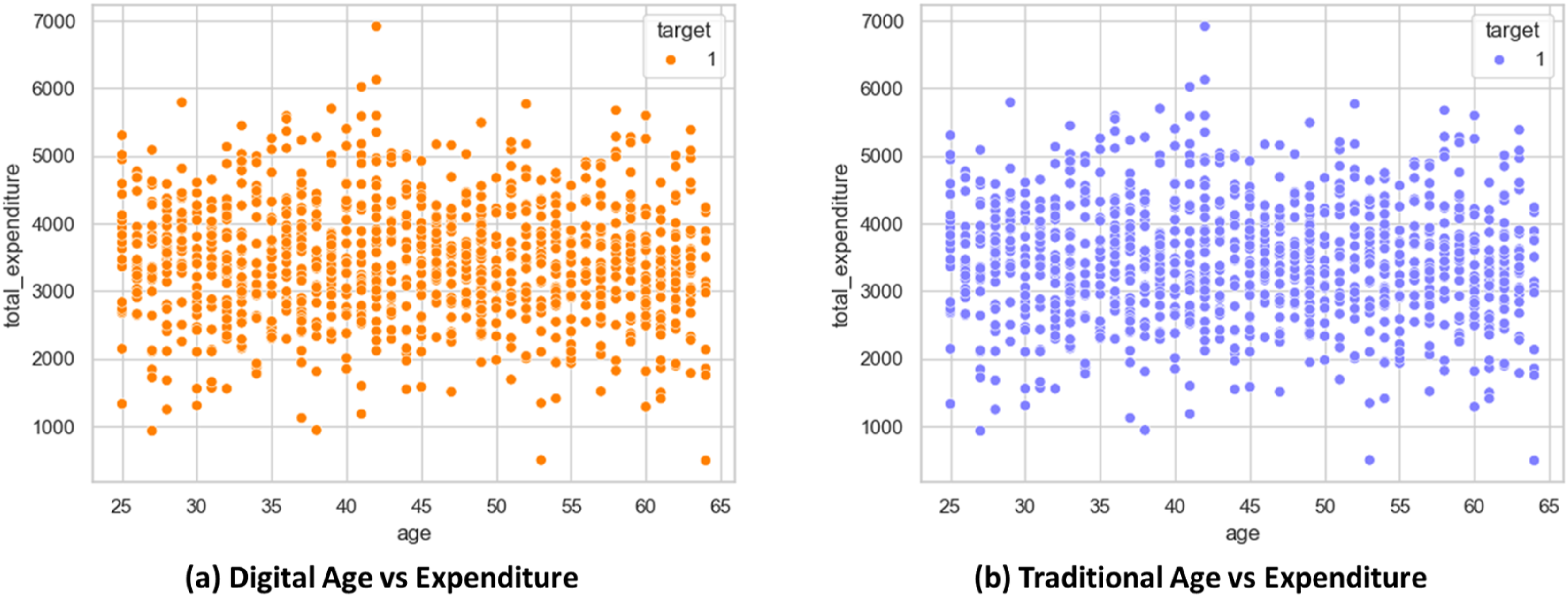

The correlation matrices for asset structures that contain digital assets and traditional assets are presented in Figure 4. It enhances the visualization of the degree of correlation and how consumption patterns and income levels tend to be related to asset types. The presence of digital assets is associated with weak correlations with expenditure behavior in Figure 4(a), indicating inconsistent patterns in consumption, while traditional asset holders demonstrate stable and income-aligned consumption behavioral patterns in Figure 4(b). Furthermore, traditional asset holders illustrated strong correlations with spending arrangements on both needs and luxury spending. Overall, these patterns emphasize the appearance of asset structures in household consumption decisions.

Figure 4.

Correlation matrices illustrating relationships between household expenditure and asset structures: (a) Digital assets, and (b) Traditional assets.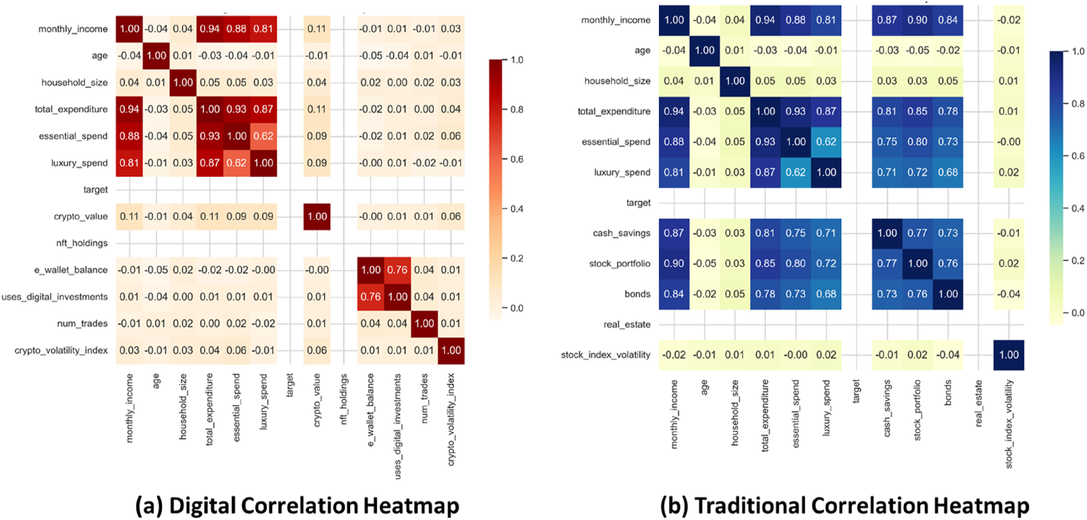

The employment status distribution in households with traditional and digital asset structures is shown in Figure 5. Both groups exhibit similar proportions across employment categories, with unemployed individuals representing the largest share at 26.3%. This consistency also facilitates balance in employment status across asset types to help reduce bias in analyzing consumption. In particular, both figures have almost the same representation of self-employed, employed, and retired individuals, which demonstrates structural consistency. Overall, this assures that any differences in consumption behavior are more likely driven by asset structure than employment status.

Figure 5.

Employment status distribution in households with (a) digital and (b) traditional asset structures.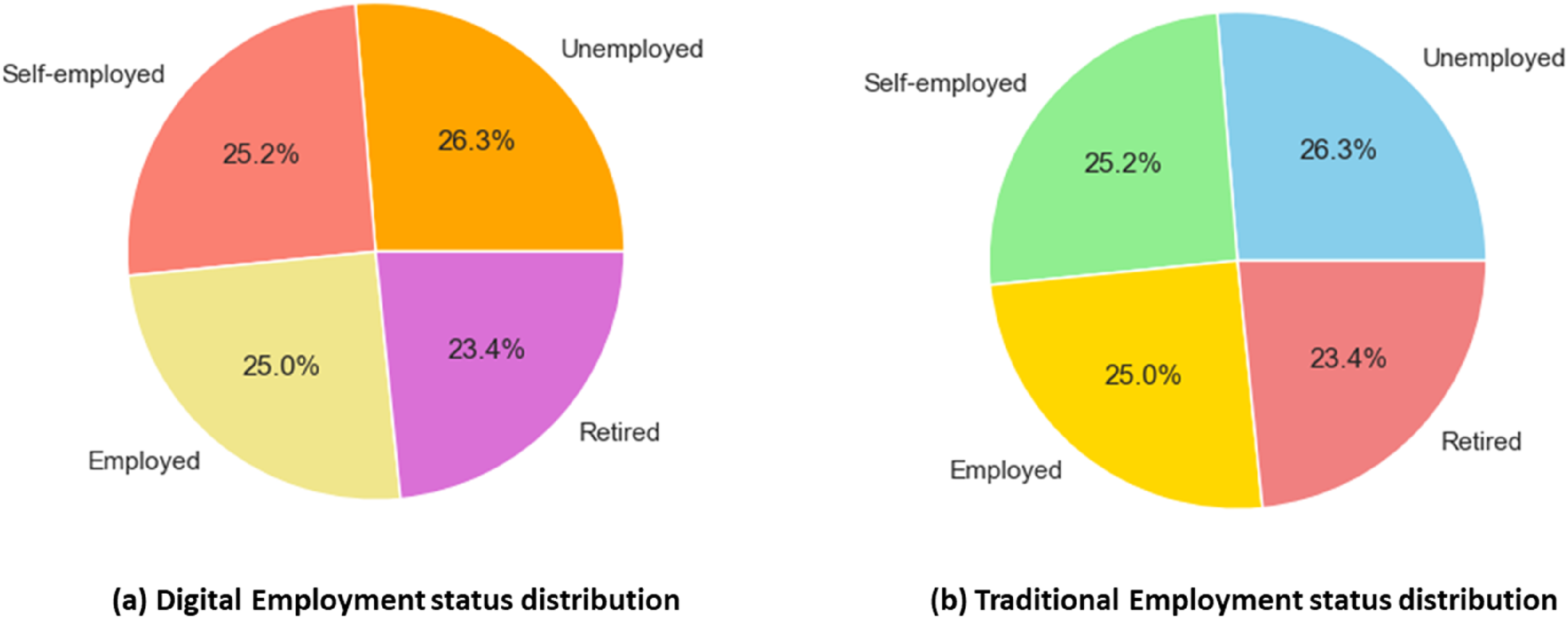

Both digital and traditional asset-structured households’ monthly average spending are shown in Figure 6. Similarly, both produce a pattern of expenditure with relatively high fluctuations about a central tendency between 2022 and 2024. In Figure 6(a), there is slightly more fluctuation, indicating that households with a digital asset structure have greater sensitivity in their spending behavior, and underscores the consumption responses to changes in exposure to digital assets. In contrast, Figure 6(b) illustrates a more stable pattern of expenditure associated with traditional asset holders that have more consistent consumption behavior. These graphics illustrate time-related variation in household expenditures based on asset structure type.

Figure 6.

Monthly average household expenditures over time for (a) households holding digital assets and (b) households holding traditional assets.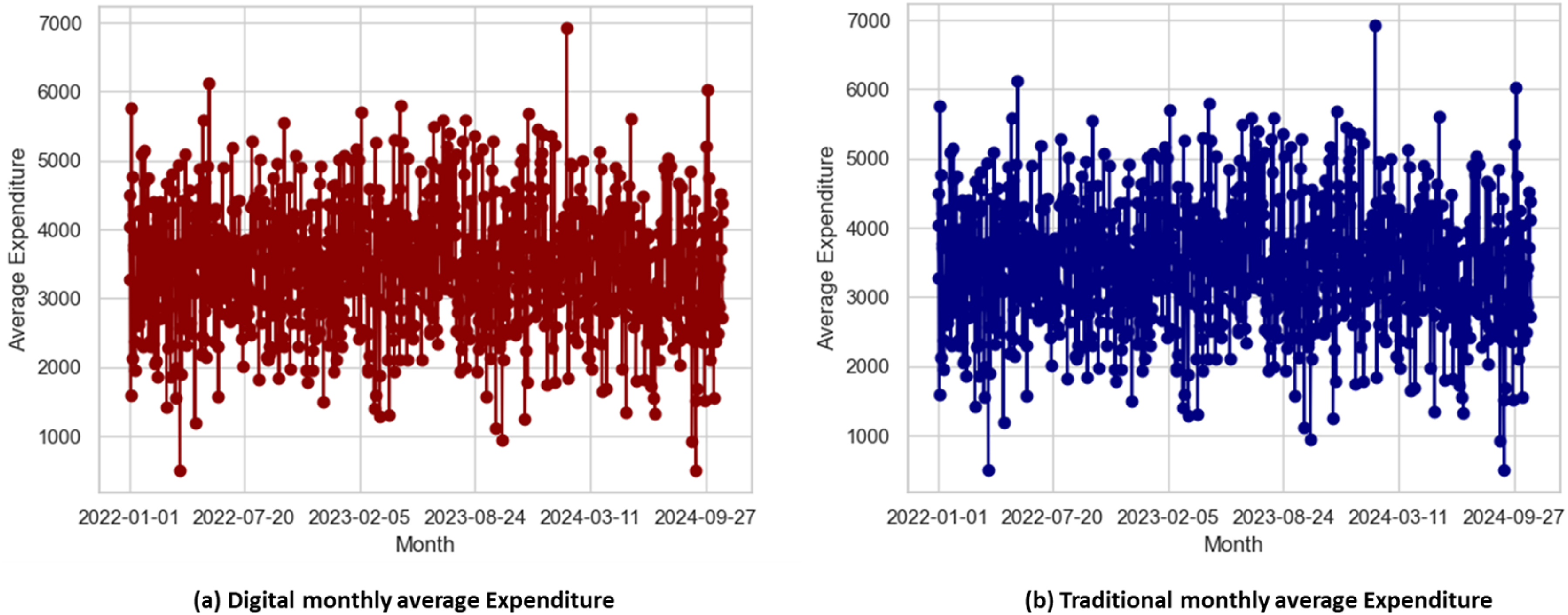

The monthly income distribution of households that decided to use digital financial assets as opposed to traditional financial assets is displayed in Figure 7. The income distributions in both figures are similar, both have right-skewed, roughly normal distributions centered about mid-income. Figure 7(a) shows a slightly higher concentration of households in the 4000–6000 income bucket, which suggests moderate digital asset adoption among middle-income earners. Figure 7(b) has a comparable distribution but slightly less spread among the income buckets, suggesting that traditional asset holders have more income stability. The visual comparison is useful and supports the goal, which is to examine the consumption patterns associated with using particular assets.

Figure 7.

Monthly income distribution of (a) Digital, and (b) Traditional Assets.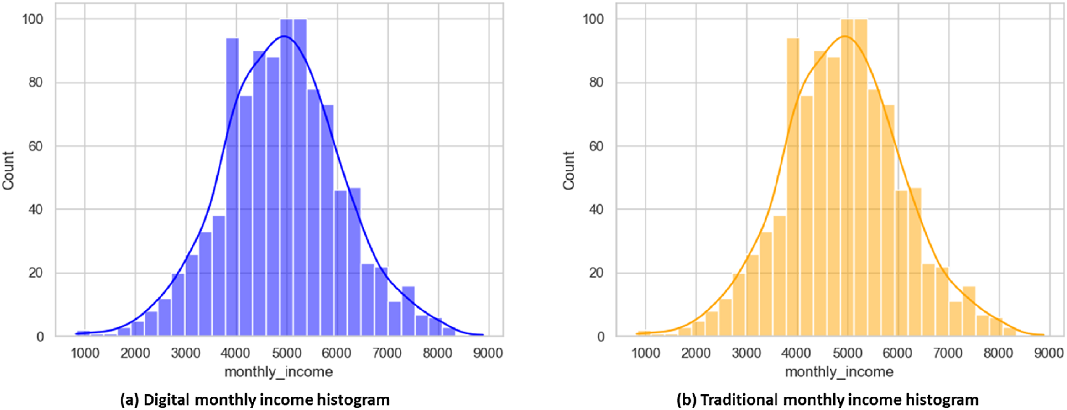

Figure 8 shows how household consumption is distributed according to types of financial assets, clearly separated into digital and traditional. Digital assets make up a greater share, accounting for 62% of total household consumption, with cryptocurrencies, digital wallets, online stock investments, and digital gold being the most utilized digital assets. Traditional assets make up 38% of total consumption, with traditional bank savings and fixed deposits being the most consumed traditional assets, alongside physical gold, real estate, and insurance. This shift demonstrates that households are developing a preference for using digital financial instruments that are increasingly influencing household consumption behaviors.

Figure 8.

Distribution of household consumption proportions attributable to (a) digital assets and (b) traditional assets.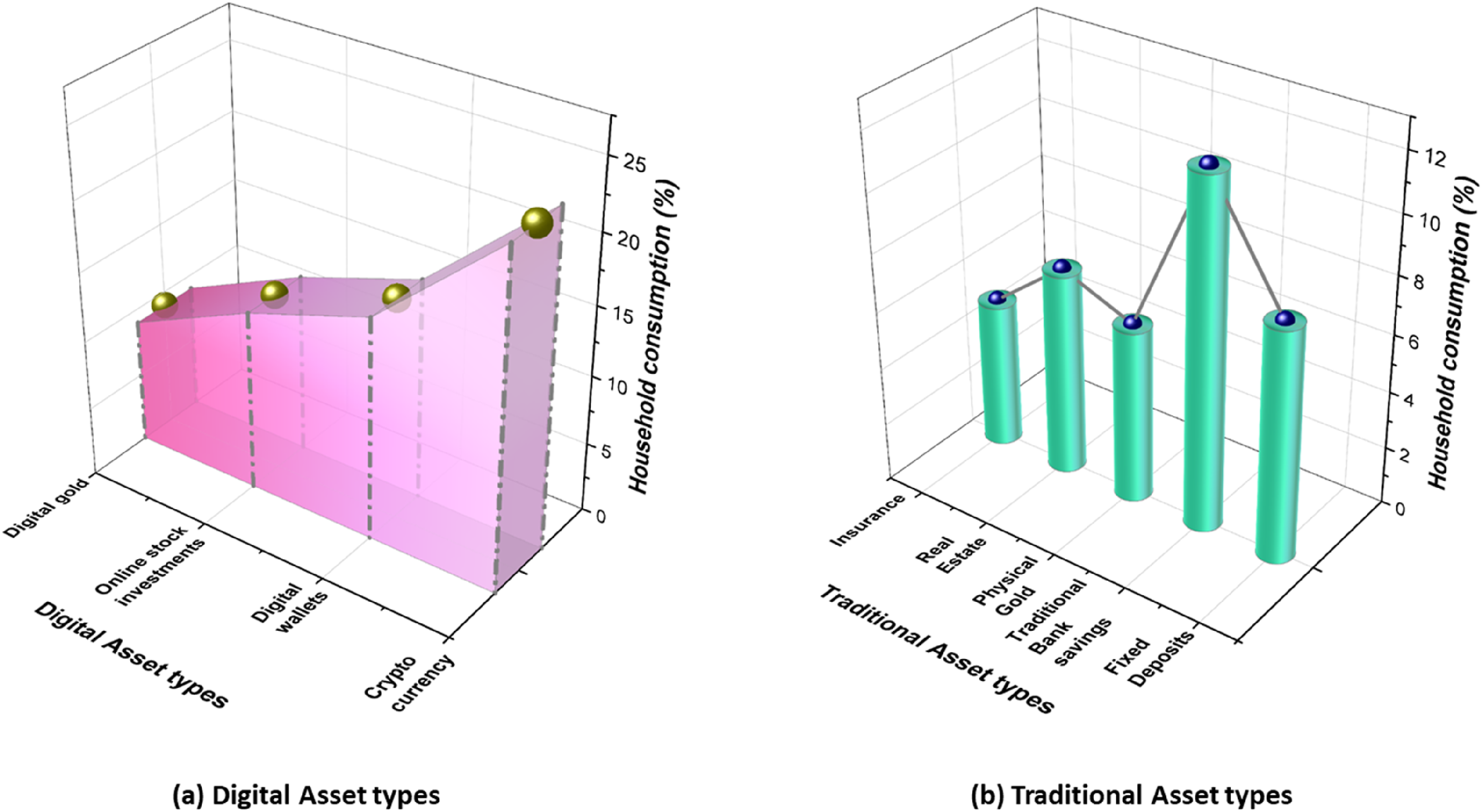

The SHAP feature impact graph serves to assess the impact of each input variable in estimating household consumption behavior based on the digital and traditional asset structures, as shown in Figure 9. This serves the purpose of discerning which financial features have the largest impact on the model’s predictions. It appears that for a digital asset structure, the crypto value and e-wallet balance have a relatively higher impact than the measures included to represent a traditional asset structure, like monthly income or bonds, which have a lower impact. It serves to support the stronger predictive relevance of digital assets when making consumption decisions. Overall, the graph indicates that the model has successfully produced emphasis on its ability to identify important nonlinear relationships.

Figure 9.

SHAP feature importance plots depicting the influence of various financial features on household consumption predictions: (a) digital asset features, and (b) traditional asset features.

Comparative analysis

The SLSTM model, while good at capturing temporal dependencies in household consumption data, often struggles with slow convergence, poor weight initialization, and limited ability to exploit the complex nonlinear dependencies in the financial system. These limitations hinder its capacity to fully appreciate the evolving relationships of consumption with respect to digital and traditional assets.

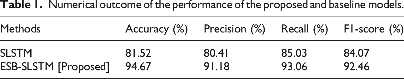
To outline the comparison of the performance of the proposed technique (ESB-SLSTM) with the baseline model (SLSTM) in evaluating the relationship between household financial asset structure and consumption decisions. Numerical results for metrics are shown in Table 1 and Figure 10. The metrics allow for validation of the effectiveness of the proposed ESB-SLSTM model in modeling complex consumption behavior associated with both traditional and digital assets.

Table 1.

Numerical outcome of the performance of the proposed and baseline models.

Methods	Accuracy (%)	Precision (%)	Recall (%)	F1-score (%)
SLSTM	81.52	80.41	85.03	84.07
ESB-SLSTM [Proposed]	94.67	91.18	93.06	92.46

Figure 10.

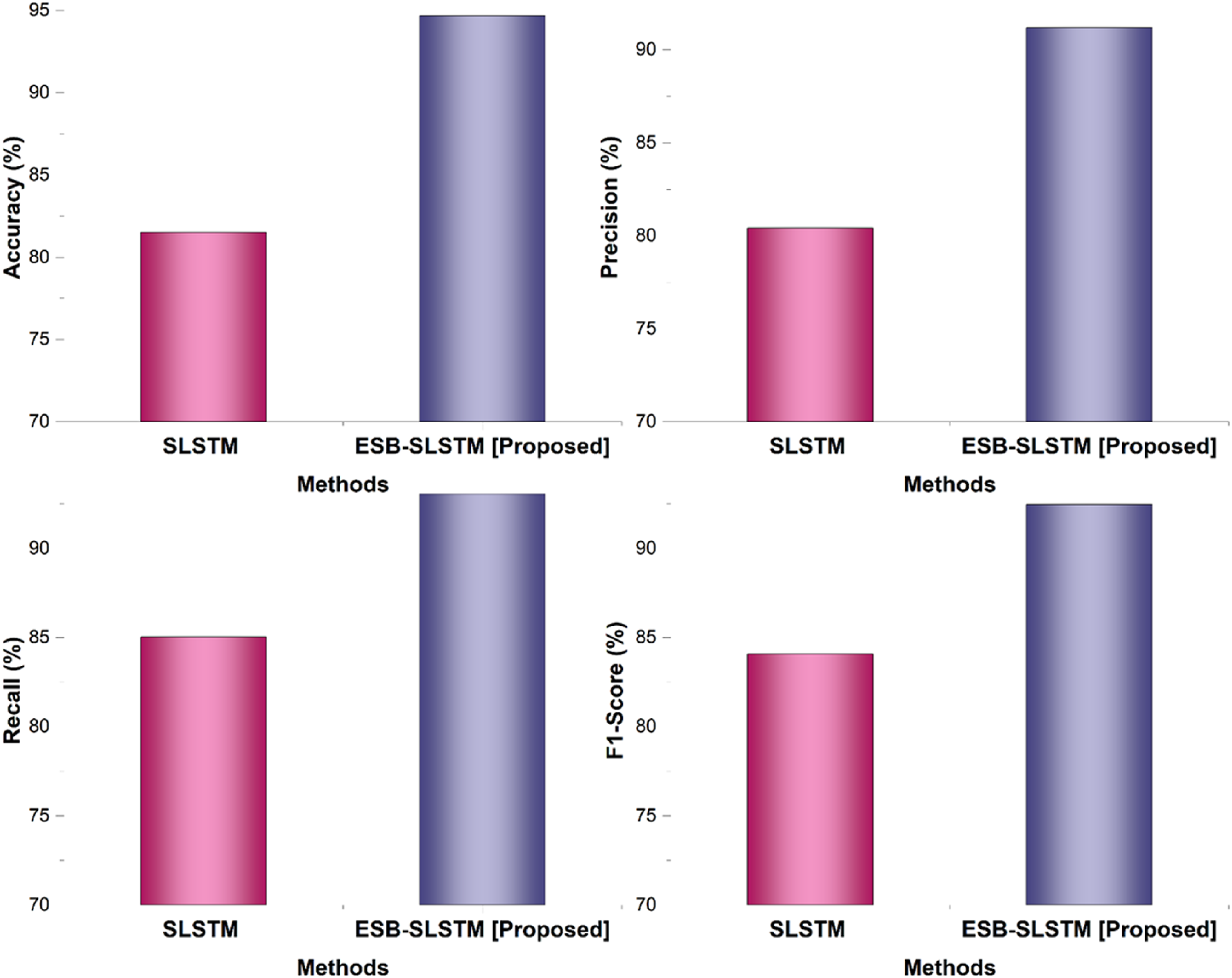
Outcome of the SLSTM and ESB-SLSTM methods.

When comparing the proposed ESB-SLSTM with the baseline SLSTM, a clear improvement is observed across four evaluation metrics. The proposed model has an accuracy approximately 13% higher than SLSTM, demonstrating greater predictive capacity. Likewise, the precision indicates an enhancement of 10.41% suggesting improved correctness in identifying the consumption behavior within a household given its asset structure. The recall has increased by 8.63%, suggesting improved market dynamics of capturing relevant household consumption patterns. Finally, the F1-score also increased by 8.39%, suggesting balanced improvements in the precision and recall metrics. In general, these results provide clear evidence that the proposed approach is superior to the baseline approach of customers’ real-life financial consumption behaviors.

To address these limitations, the proposed ESB-SLSTM combines the ESB optimization algorithm with the SLSTM architecture. This hybrid approach increases convergence speed, facilitates parameter tuning, and increases the learning capacity to capture complex, nonlinear relationships among asset structures and household behavior. The ESB component guides a model to escape local minima, produces a better fit, and makes more accurate predictions. It also enhances the model’s sensitivity to change in digital asset holdings, and thus provides a more sensitive and flexible modeling of customers’ real-life financial consumption behaviors. Due to its flexibility, ESB-SLSTM is a powerful and intelligent approach to decision-making in the era of digital finance.

The findings of this study, while robust within the modeled context, must be considered in light of the China-specific dataset. China’s unique economic landscape, characterized by rapid digitalization led by tech giants like Alibaba and Tencent, a high household savings rate, and specific regulatory frameworks for digital assets, may limit the direct generalizability of the model to other countries with different financial ecosystems, cultural attitudes toward debt and consumption, and levels of fintech adoption. For instance, the strong impact of e-wallet balances identified in our model may be less pronounced in economies where traditional banking is more dominant. Future research should aim to validate the ESB-SLSTM framework on multinational datasets to develop a more universal model of digital asset-driven consumption behavior. This would help identify which relationships are fundamental to household economics and which are specific to regional economic structures.

Conclusion

In the new digital economy, understanding how changing financial asset structures affect household consumption is necessary to formulate policy and planning. The objective of this research was to analyze the effects of both traditional and digital financial assets on household consumption decisions using sophisticated deep learning methods. The dataset consisted of household-level asset and consumption information that included parameters such as income, demographic factors, monthly spending, and asset types from finance surveys. Data pre-processing involved handling missing values, outlier detection, and performing z-score standardization to standardize the input features. A new model, Enriched Satin Bowerbird mutated Stacked Long Short-Term Memory (ESB-SLSTM), was developed to deal with the temporal and nonlinear features of financial behavior. The ESB-SLSTM model was developed in Python, with accuracy (94.67%), precision (91.18%), recall (93.06%), and F1-score (92.46%) that significantly outperformed the baseline SLSTM models. This research doesn’t consider real-time market volatility or external macroeconomic shocks that may be directly influencing household consumption decisions in real time, in addition to asset structures. Future models may include real-time financial indicators (such as interest rates, inflation trends, or cryptocurrency volatility indexes) as additional input features. This would increase the model’s received responsiveness to external financial shocks and diminish predictive robustness in stochastic economic environments. This research is highly applicable in the financial planning and fintech industries because household consumption behavior is useful in conceptualizing personalized financial products and services. Digital banks and investment advisory services will also benefit because they can provide predictive insights associated with different asset structures.

Footnotes

ORCID iD

Xingcai Yao

Funding

The authors received no financial support for the research, authorship, and/or publication of this article.

Declaration of conflicting interests

The authors declared no potential conflicts of interest with respect to the research, authorship, and/or publication of this article.

Data Availability Statement

The authors declare that the data supporting the findings of this study are available within the article. The raw/derived data supporting the findings of this study are available from the corresponding author at request.*

Appendix

References

Peng

Robinson

Zheng

, et al. The limits of livelihood diversification and sustainable household well-being, evidence from China. Environ Dev 2022; 43: 100736.

Cho

Kim

. Smart homes support the wellness of one or two-person households. Sensors 2022; 22(20): 7816.

Balasoiu

Chifu

Oancea

. Impact of direct taxation on economic growth: empirical evidence based on panel data regression analysis at the level of EU countries. Sustainability 2023; 15(9): 7146.

Zheng

Dang

Assad

. Household energy consumption, energy efficiency, and household income–Evidence from China. Appl Energy 2024; 353: 122074.

Dushi

Trenkamp

Bee

, et al. Measuring income of the aged in household surveys: evidence from linked administrative records. J Pension Econ Finance 2025; 24(1): 95–122.

Gajdzik

Jaciow

Hoffmann-Burdzińska

, et al. Impact of economic awareness on sustainable energy consumption: results of research in a segment of Polish households. Energies 2024; 17(11): 2483.

Jiao

Chen

, et al. Social security, relative deprivation, digital capacity, and household financial investment behavior. Int Rev Financ Anal 2024; 96: 103771.

Yannelis

Amato

. Household behavior (consumption, credit, and investments) during the COVID-19 pandemic. Annu Rev Financ Econ 2023; 15(1): 91–113.

Kumari

Bala

Chakraborty

. An empirical study of user adoption of cryptocurrency using blockchain technology: analysing role of success factors like technology awareness and financial literacy. J TheoreAppl Elect Comm Res 2023; 18(3): 1580–1600.

10.

Mustafa

Islam

Asyraf

, et al. The effects of financial attitudes, financial literacy, and health literacy on sustainable financial retirement planning: the moderating role of the financial advisor. Sustainability 2023; 15(3): 2677.

11.

Harahap

Thoyib

Sumiati

, et al. The impact of financial literacy on retirement planning with serial mediation of financial risk tolerance and saving behavior: evidence from medium entrepreneurs in Indonesia. Int J Financ Stud 2022; 10(3): 66.

12.

Yin

Liu

, et al. A study of the impact of digital finance usage on household consumption upgrading: based on a financial asset allocation perspective. Int Rev Econ Finance 2024; 96: 103628.

13.

Shang

Yan

Zhang

, et al. Digital financial asset price fluctuation forecasting in digital economy era using blockchain information: a reconstructed dynamic-bound Levenberg–Marquardt neural-network approach. Expert Syst Appl 2023; 228: 120329.

14.

Liu

. Artificial intelligence development and household financial asset allocation. Int Rev Econ Finance 2025; 28: 104365.

15.

Ahmadi

Soofiabadi

Nikpour

, et al. Developing a deep neural network with fuzzy wavelets and integrating an inline PSO to predict energy consumption patterns in urban buildings. Mathematics 2022; 10(8): 1270.

16.

Huang

Liu

Xue

, et al. Imbalanced credit card fraud detection data: a solution based on hybrid neural network and clustering-based undersampling technique. Appl Soft Comput 2024; 154: 111368.

17.

Liu

, et al. The analysis of credit risks in an agricultural supply chain finance assessment model based on genetic algorithm and backpropagation neural network. Comput Econ 2022; 60(4): 1269–1292.

18.

Tripathi

Sharma

. Modeling bitcoin prices using signal processing methods, Bayesian optimization, and deep neural networks. Comput Econ 2023; 62(4): 1919–1945.

19.

Chen

Long

. E-commerce enterprises’ financial risk prediction based on FA-PSO-LSTM neural network deep learning model. Sustainability 2023; 15(7): 5882.

20.

Qian

Gao

, et al. Soft reordering one-dimensional convolutional neural network for credit scoring. Knowl Base Syst 2023; 266: 110414.

21.

Aydin

Sahin

Deveci

, et al. Prediction of financial distress of companies with artificial neural networks and decision tree models. Mach Learn Appl 2022; 10: 100432.

22.

Mousapour Mamoudan

Ostadi

Pourkhodabakhsh

, et al. Hybrid neural network-based metaheuristics for prediction of financial markets: a case study on the global gold market. J Comp Desig Eng 2023; 10(3): 1110–1125.

23.

Dube

Nzimande

Muzindutsi

. Application of artificial neural networks in predicting financial distress in the JSE financial services and manufacturing companies. J Sustain Finance Invest 2023; 13(1): 723–743.

24.

Di Lorenzo

Piscopo

Sibillo

. Addressing the economic and demographic complexity via a neural network approach: risk measures for reverse mortgages. Comput Manag Sci 2024; 21(1): 11.

25.

Konak

Bülbül

Türkoǧlu

. Feature selection and hyperparameters optimization employing a hybrid model based on genetic algorithm and artificial neural network: forecasting dividend payout ratio. Comput Econ 2024; 63(4): 1673–1693.

26.

Magazzino

Mele

Santeramo

. Using an artificial neural network experiment to assess the links among financial development and growth in agriculture. Sustainability 2021; 13(5): 2828.