Data and dimension reduction for visual financial performance analysis

Abstract

This article assesses the suitability of data and dimension reduction methods, and data–dimension reduction combinations, for visual financial performance analysis. Motivated by no comparable quantitative measure of all aspects of dimension reductions, this article attempts to capture the suitability of methods for the task through a qualitative comparison and illustrative experiments. While the discussion deals with differences of data–dimension reduction combinations in terms of their properties, the experiments illustrate their general applicability for financial performance analysis. The main conclusion is that topology-preserving data–dimension reduction combinations with predefined, regular grid shapes, such as the self-organizing map, are ideal tools for this task. We illustrate advantages of these types of methods with a visual financial performance analysis of large European banks.

Keywords

Financial performance analysis visualization data reduction dimension reduction

Introduction

The ongoing global financial crisis and European debt crisis have highlighted the importance of a thorough understanding of financial entities, be they economies, markets, or institutions. Fortunately, rapid advances in information technology have enabled access to huge databases of financial information. Unfortunately, analyzing these data is not completely unproblematic. Except for incompleteness of data due to missing values and comparability issues due to reporting differences,¹ as well as outliers and skewed distributions,² the multidimensionality of the problem is a central challenge for comprehension. In the case of firm-level financial entities, performance can be measured along several subdimensions, such as asset and management quality, as well as capital adequacy, earning performance, and liquidity ratios. Factors that further complicate the assessment of these high-dimensional and large-volume data are temporal and cross-sectional dependencies and relations. Generally, performance analysis of banks can be attempted with various aims, such as studies on determinants of entity performance,³ predictions of undesired entity-level events,⁴ and efficiency measurement of entities.⁵ While a wide range of methods have been applied to fulfill these aims, they seldom focus on providing the end user with representations of data in easily understandable formats. A visualization or abstraction of high-dimensional data supports the knowledge crystallization process by enabling utilization of the pattern recognition capabilities of the human brain for exploring structures in databases.

Data and dimension reduction techniques, and their combination for data–dimension reduction (DDR), obviously hold some promise for representing data in an easily understandable format. Data reductions provide overviews of data by compressing information, whereas dimension reductions provide low-dimensional overviews of similarity relations in data. While the quality of data reductions can be quantified by common evaluation measures such as quantization error, assessing the superiority of one dimension reduction method over others with a quantitative measure is more difficult.

Since the mid-20th century, the overload of available data has stimulated a soar in the development of dimension reduction methods with inherent differences. Most of the methods fall into those aiming at distance and topology preservation (for an overview, see section “Related literature” and Lee and Verleysen⁶). The distance-preserving methods have their basis in those preserving spatial distances in the dataset (e.g. the family of multidimensional scaling (MDS) methods), while topology-preserving methods have their basis in those preserving neighborhood relations in the dataset (e.g. the self-organizing map (SOM)).⁷ However, most differences in the quality of dimension reductions, as all structural information can impossibly be preserved in a lower dimension, derive from variations in preserved similarity relations (i.e. objective function), such as pairwise distances or topological relationships. The performance, and choice of model specification, of one method can generally be motivated by its own quantitative quality measure. However, the relative goodness of different methods depends strongly on the correspondence between the particular measure and the objective function.

The large number of dimension reduction methods has obviously stimulated quality comparisons along different measures. However, despite many attempts, inconsistency of the comparisons has led to no unanimity on the superiority of one method.^8–10 This also verifies that the goodness of methods depends to a large extent on the correspondence between the measure and the objective function and further confirms that the quality measure is a user-specified parameter depending on the task at hand. While recent advances in unified measures for evaluating dimension reductions have included a parameter for the user to specify properties that are more important to be preserved,^11,12 quantitative measures still have difficulties in including qualitative differences in properties of methods, such as differences in flexibility for difficult data and the shape of the low-dimensional output. This motivates assessing the suitability of data and dimension reduction methods for a specific task from a qualitative perspective.

The main aim of this article is to capture the most suitable methods for visual financial performance analysis according to the needs for the task. To date, the most popular method for the task has been the SOM, which is oftentimes asserted as an artifact of its simplicity and intuitive formulation.^6,13 Yet, being well known or simple, while being an asset, is not a proper validation of relative goodness. Hence, we assess the suitability of three classical, or so-called first-generation, dimension reduction methods for financial performance analysis: metric MDS,¹⁴ Sammon’s¹⁵ mapping, and the SOM. Rather than being the most recent methods, the rationale for comparing these methods is to capture the suitability of well-known dimension reduction methods with inherently different aims: global and local distance preservation and topology preservation. For DDR, we test serial and parallel combinations of the projections with three data reduction or compression methods: vector quantization (VQ),¹⁶ k-means clustering,¹⁷ and Ward’s¹⁸ hierarchical clustering. The relative goodness of methods for financial performance analysis is first discussed from a qualitative perspective, in particular with respect to the needs for the task at hand. That is, building low-dimensional mappings from high-dimensional and large-volume data that function as displays for additional visualizations, be it individual data (e.g. time series of entities), structural properties of the data (e.g. distance structures and densities), or qualities of the models (e.g. distortions). Specifically, we classify this into four key criteria: form of structure preservation, computational cost, flexibility for problematic data, and shape of the output. Then, experiments on a dataset of annual financial ratios for European banks are used to illustrate the general applicability of the DDR combinations for the task. Results of these comparisons are then projected to the second generation of dimension reduction methods for a final, more general discussion on the superiority of methods for visual financial performance analysis.

This article is structured as follows. In section “Related literature,” we review the literature related to financial performance analysis and data and dimension reduction. While section “Methodology” briefly introduces the data and dimension reduction methods used in this article, section “DDR combinations for the task at hand” discusses optimal DDR combinations for financial performance analysis and disentangles the needs and aims into concrete properties for measuring suitability. Section “Qualitative and quantitative experiments” compares data and dimension reduction methods for financial performance analysis by a qualitative discussion, presents the financial dataset, and shows some illustrative experiments. Section “Discussion” discusses critically the results and draws parallels with the second generation of dimension reduction methods. Finally, section “Conclusion” concludes by presenting key findings and suggestions for future work.

Related literature

This section reviews related literature from three distinct directions. We discuss the literature related to measuring financial performance of banks, present a brief taxonomy and review of data and dimension reduction methods, and finally discuss comparisons of data and dimension reductions.

Financial performance analysis of banks

Measuring performance of banks is a common task and has been performed with a wide variety of methods and aims. Depending on the definition of “performance,” different methods have been applied for assessing and measuring characteristics of banks. The complexity is further increased as one may also be interested in properties of entities across cross sections and their evolution over time. We approach the literature from three angles. Thereafter, we give an outlook on visualizing bank-related data.

First, there is a broad literature on determinants of bank performance. These types of studies have mostly utilized high-dimensional data and conventional statistical techniques.^3,19 Second, a large number of studies have created early-warning models in attempts to predict future distress in bank performance of two forms: country-specific banking crises²⁰ and bank-specific bank distress.^21–23 Recently, some advances in predictive capabilities have been gained through nonparametric methods.⁴ Third, there is a field on its own on measuring the efficiency of individual banks. This has most commonly been performed with data envelopment analysis,⁵ fuzzy set theory,²⁴ and gray relational analysis.²⁵ Even though there is no one method that is suited for every purpose and situation, the above methods do not even propose to be applicable for visual performance analysis.

Visualization of bank-related data concerns a wide range of approaches, such as network models for illustrating interconnectedness, extended plots for assessing raw data or their summaries, and analytical methods. Following the proposition by Aigner et al.²⁶ on a better integration of visual, analytical, and user-centered methods, the focus herein is on visualization through analytical methods for data and dimension reduction. Dimension reduction methods, while not being highly common for visualization in financial analysis, have previously been employed for visual financial performance analysis. MDS and the SOM have been applied in illustrating the performance of banks on a low-dimensional display: MDS was used for illustrating the performance of Spanish banks²⁷ and the SOM was used for benchmarking European banks.²⁸ In addition, while there exist applications of both MDS²⁹ and the SOM³⁰ for predicting failures of banks, the SOM has retained its popularity not only in the domain of bank analysis but also in other financial areas. Some examples of financial application areas of the SOM are firm-level analysis of the pulp and paper industry³¹ and country-level analysis for financial stability surveillance.³³

Data and dimension reduction methods

The first dimension reduction methods date back to the early 20th century. However, only since the 1990s has there been a significant soar in the number of developed dimension reduction methods. We use that as a cutting point for dividing the methods into first- and second-generation methods. The first generation consists of the well-known classical methods that are still broadly used and accepted in a wide range of domains. Drawing upon the first introduced, but still commonly used, variance-preserving principal component analysis (PCA),³⁴ an entire family of distance-preserving MDS-based methods has been developed. PCA uses an orthogonal transformation to convert a set of possibly correlated variables into a smaller set of linearly uncorrelated variables called principal components. Classical metric MDS, as proposed by Young and Householder³⁵ and Torgerson,¹⁴ is a counterpart to PCA, which addresses the same problem but aims instead at preserving pairwise distances between data. Nonlinear versions are the first introduced nonmetric MDS by Shepard³⁶ and Kruskal³⁷ and the later developed Sammon’s¹⁵ mapping. The topology-preserving family of methods was launched through the introduction of the SOM.⁷ The SOM differs by reducing both dimensions and data through a neighborhood-preserving vector quantification.

The second generation is a less homogeneous group of methods ranging from spectral techniques to graph embedding. A soar in developed methods at the turn of the century led to several innovative techniques, such as curvilinear component analysis (CCA),³⁷ curvilinear distance analysis (CDA),³⁸ local MDS (LMDS),^38,39 generative topographic mapping (GTM),^40,93 locally linear embedding (LLE),⁴² Isomap,⁴³ Laplacian eigenmaps (LE),⁴⁴ and maximum variance unfolding (MVU).⁴⁵ Some more recent methods are, for instance, t-distributed stochastic neighbor embedding (t-SNE)⁴⁶ and exploration observation machine (XOM).⁴⁷ It is worth to note that the second-generation techniques, while introducing novel approaches to processing data, are oftentimes developed out of the idea that the global distance metric structure of the data might be relaxed, yet not always with a focus on topology.

In addition to two generations, dimension reduction methods can also be illustrated in a tree-structured taxonomy. The tree structure in Figure 1 is a nonexhaustive taxonomy of dimension reduction methods derived from that in Lee and Verleysen (p. 234).⁶ While the focus herein is on methods based upon geometrical concepts, there exists also other methods, such as those based upon auto-associative neural networks (AANNs). The tree structure ends with some exemplifying techniques, where first-generation methods are differentiated from second-generation methods through a gray background. Methods can roughly be divided into those aiming at distance and topology preservation. The distance-preserving methods can still be divided based on different distances, such as spatial (e.g. PCA, MDS, Sammon’s mapping, CCA), and LMDS), graph (e.g. Isomap and CDA), and other (e.g. MVU). Topology-preserving methods can be divided into those with a predefined grid shape (e.g. SOM, GTM, and XOM) and those without (e.g. LLE, LE, and t-SNE). Thus, Figure 1 illustrates a number of categorizations, such as a focus on geometrical versus other concepts, distance versus topology preservation, spatial versus graph versus other distances, and predefined versus data-driven grid shapes. As noted about the taxonomy, the categorization is also incomplete. Examples of additional categories are continuous versus discrete mappings, optional versus mandatory data reductions, linear versus nonlinear mappings, and implicit versus explicit mappings.

Figure 1.

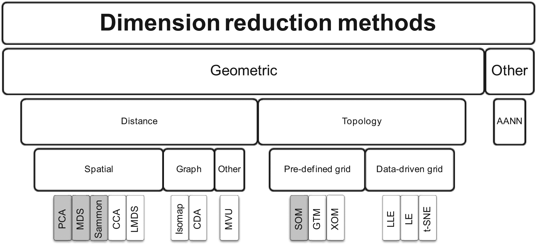
A taxonomy of dimension reduction methods.

Although there is no common taxonomy of data reduction methods, several properties can be used for differentiating between methods: soft versus hard clustering, hierarchical versus nonhierarchical methods, and monothetic versus polythetic goals, for instance. While soft clustering reduces data by assigning them to each cluster to a certain degree, hard clustering either assigns data to a cluster or does not. Hierarchical methods (e.g. Ward’s method¹⁸) produce a taxonomy of cluster structures, in which small child clusters are also nested within larger parent clusters and may be divided into agglomerative (bottom-up) and divisive (top-down) approaches. Nonhierarchical methods approach data reduction from numerous different angles and may roughly be divided into centroid-based (e.g. k-means¹⁷ and VQ¹⁶), distribution-based (e.g. expectation–maximization algorithm⁴⁸), and density-based clustering (e.g. DBSCAN⁴⁹). The differences between monothetic versus polythetic methods relate mainly to hierarchical clustering, where the former uses the inputs one by one and the latter all the inputs at once.

Comparisons of data and dimension reductions

When reviewing the literature on method comparisons, we first focus on dimension reduction methods and then on data reduction methods. The focus is on neutral evaluations of methods rather than evaluations in articles presenting novel methods. While articles presenting novel methods generally include an evaluation and conclude at least partial superiority of the invented method, such as some of the ones presented in section “Data and dimension reduction methods,” they may be biased to a lesser or greater extent toward data and evaluation measures suitable for that particular method.

The large number of methods has obviously also stimulated a large number of performance comparisons between them. The comparisons mainly vary in terms of used data and evaluation measures, whereas there may also be some variation in the precise utilization of methods. For instance, Flexer^8,9 used Pearson correlation, Duch and Naud⁵⁰ hypercubes in three to five dimensions, and Bezdek and Pal⁵¹ the metric topology-preserving index to show that MDS outperforms the SOM. Trosset¹³ argues that a serial combination of clustering and MDS is superior to the SOM. Venna and Kaski¹⁰ and Nikkilä et al.⁵² show superiority of the SOM and GTM in terms of trustworthiness of neighborhood relationships, while later Himberg⁵³ and Venna and Kaski⁵⁴ show superiority of CCA in terms of the same measure. Not surprisingly, De Vel et al.⁵⁵ show, using Procrustes analysis and Spearman’s rank correlation coefficients on various datasets, that the superiority of a method depends on the used evaluation measures and data.

Recently, Lee and Verleysen¹¹ proposed a unified measure based upon a coranking matrix for evaluating dimension reductions, a good starting point for generic evaluations. Lueks et al.¹² further developed the measure by letting the user specify the properties that are more important to be preserved. While being useful aids in comparing methods, they neither show nor propose existence of one superior method for every type of data and preferences of similarity preservation. Hence, despite many attempts, inconsistent comparisons result in no conclusion on the superiority of one method.

When reviewing the literature on methods for data reduction, one can easily observe that there is no unanimity on the best available method. Herein, the focus is on comparisons between methods performing DDR and stand-alone data reduction methods. Bação et al.⁵⁶ show that the SOM outperforms k-means clustering with three evaluation measures and four datasets. Flexer^8,9 shows that k-means clustering outperforms the SOM using a Rand index and 36 datasets. Waller et al.⁵⁷ show on 2580 datasets that the SOM performs equally well with k-means clustering and better than other methods. Balakrishnan et al.⁵⁸ show that k-means outperforms the SOM on 108 datasets, but do not decrease the SOM neighborhood to zero at the end of learning (as, for example, Kohonen⁵⁹ proposes). Vesanto and Alhoniemi⁶⁰ showed on three datasets that two-level clustering of the SOM is equally accurate as agglomerative and partitive methods, while being computationally cheaper and having merits in visualizing relations in data. Ultsch and Vetter⁶¹ compare the SOM with hierarchical and k-means clustering and conclude that the SOM not only provides an equally accurate result but also an easily interpretable output. Despite no unanimity on superiority, the literature still indicates that the SOM and its adaptations are equally considerable alternatives for data reduction as other methods, such as centroid-based and hierarchical clustering.

Methodology

This section discusses the functioning and technical details of the data and dimension reduction methods compared in this article. The dimension reduction methods are chosen based upon three reasons: they generally cover (1) the first-generation methods, (2) the above-discussed categorizations of techniques, and (3) the previously applied techniques in this field. In this vein, this section introduces three dimension reduction methods: metric MDS, Sammon’s mapping, and the SOM.

The methods for data reduction are, on the other hand, chosen as to their resemblance to the clustering of the SOM and their suitability for data compression of dimension reductions. Again, we focus on three methods: VQ, k-means clustering, and Ward’s hierarchical clustering. VQ and k-means resemble the functioning of the prototype-based clustering of the SOM. Agglomeration of hierarchical clustering, while differing from the data compression of VQ, is suitable for DDR as its agglomeration can be restricted by neighborhood relations of a dimension reduction and adapted to account for cluster size. This section sets a starting point for the comparative discussion by introducing the methods with an emphasis on their objective functions. In the sequel, even if not always mentioned, all distances are treated as Euclidean.

Dimension reduction methods

Dimension reductions employed in this article have their basis in the first-generation methods. The main basis of classical methods is in the family of MDS-based projections. We first turn to a distance-preserving counterpart of PCA, classical metric MDS.^14,35 Due to its linearity constraints, we also turn to a nonlinear MDS-based method, Sammon’s¹⁵ mapping. That is, the aim is to project high-dimensional data $x_{j}$ to a two-dimensional (2D) data vector $y_{j}$ by preserving distances. While the aim and focus herein are on projections to two dimensions, it is worth noting that most projections are not limited by such restrictions. Let the distance in the input space between $x_{j}$ and $x_{h}$ be denoted $d_{x} (j, h)$ and the distance in the output space between $y_{j}$ and $y_{h}$ be denoted $d_{y} (j, h)$ . This gives us the objective function of metric MDS

E_{MDS} = \sum_{j \neq h} {(d_{x} (j, h) - d_{y} (j, h))}^{2}

(1)

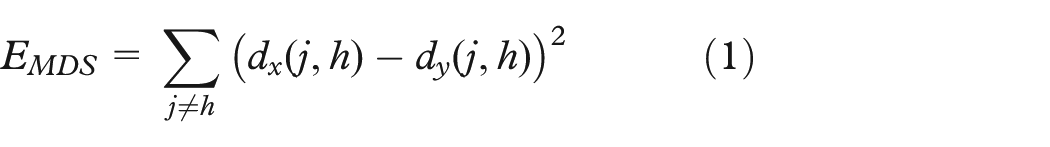
Sammon’s mapping is an MDS method in that it also attempts to preserve pairwise distances between data but differs by focusing on local distances relative to larger ones. The square error objective function for Sammon’s mapping is

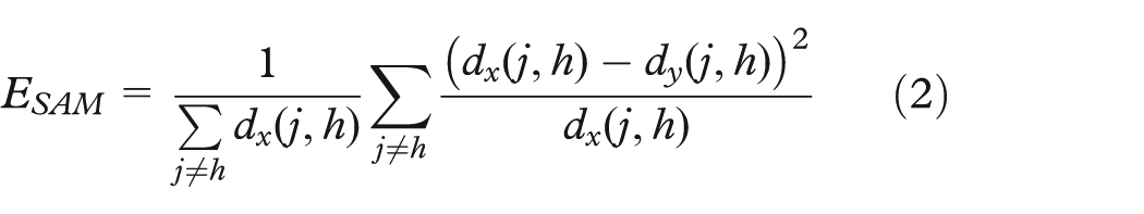
E_{SAM} = \frac{1}{\sum_{j \neq h} d_{x} (j, h)} \sum_{j \neq h} \frac{{(d_{x} (j, h) - d_{y} (j, h))}^{2}}{d_{x} (j, h)}

(2)

and shows that it considers all pairs (j, h) normalized with the distance in the original space $d_{x} (j, h)$ and weighted with $1 / d_{x} (j, h)$ . The objective functions of MDS-based methods are optimized with an iterative steepest-descent process.

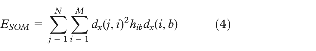
The SOM⁷ differs by reducing both dimensions and data through a neighborhood-preserving VQ. In particular, the sequential SOM can be seen as a spatially constrained form of VQ. We follow, however, the batch SOM algorithm that can instead be seen as a spatially constrained counterpart of k-means clustering. The training algorithm proceeds according to two steps: (1) finding the best-matching units (BMUs) and (2) adjusting the prototype vectors $m_{i}$ . To find $\min (d_{x} (j, i))$ , the first step assigns the input data x_j (where j = 1, 2, …, N) to their BMU $m_{b} \in m_{i}$ (where i = 1, 2, …, M). Hence, data $x_{j}$ are projected to an equidimensional prototype vector $m_{i}$ , not a 2D vector as in MDS. The second step adjusts each m_i with the batch updating algorithm

m_{i} (t + 1) = \frac{\sum_{j = 1}^{N} h_{ib (j)} (t) x_{j}}{\sum_{j = 1}^{N} h_{ib (j)} (t)}

(3)

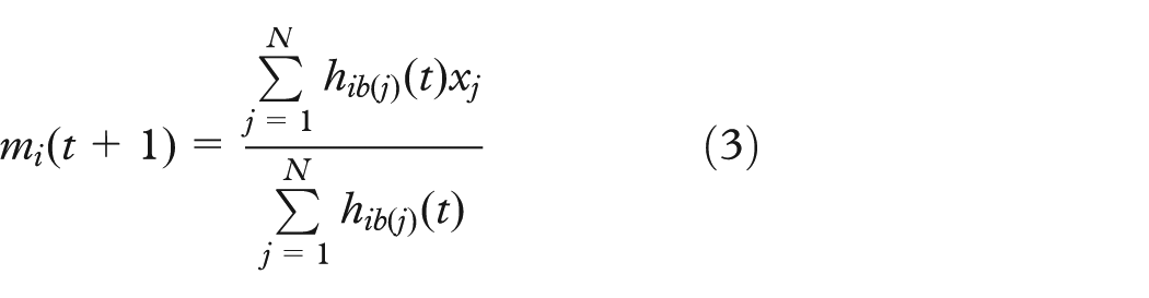
where t is a discrete time coordinate and the neighborhood $h_{ib (j)}$ is often some decreasing function of neighborhood radii and time.

Mathematical treatment of the SOM has, however, shown to be difficult. Despite an extensive discussion of the form and existence of an objective function, the literature has still not provided one for the general case.⁶² It is, however, clear that a decomposed distortion measure illustrates the learning of the SOM (a discrete form with a fixed neighborhood of that suggested in Lampinen and Oja⁶³)

E_{SOM} = \sum_{j = 1}^{N} \sum_{i = 1}^{M} d_{x} {(j, i)}^{2} h_{ib} d_{x} (i, b)

(4)

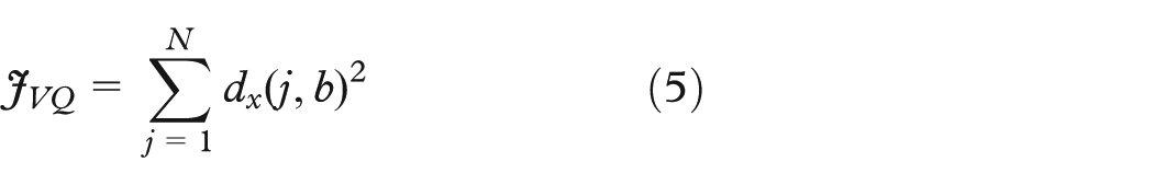
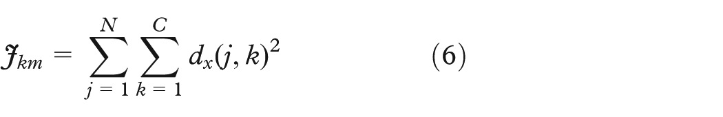
Data reduction methods

Data reduction and compression, or clustering, methods can be used for dividing data or prototypes into homogeneous groups. First, we introduce two clustering counterparts of the SOM. The sequential and batch SOMs can be seen as spatial counterparts of two prototype-based clustering methods: VQ¹⁶ and k-means clustering,¹⁷ respectively. VQ attempts to model the probability density functions in data x_j by prototype vectors m_i. As the SOM, it uses $\min (d_{x} (j, i))$ for finding the BMU for x_j, but then updates only the BMU toward the data vector. Hence, it attempts to minimize the standard squared error function or quantization error

J_{VQ} = \sum_{j = 1}^{N} d_{x} {(j, b)}^{2}

(5)

The k-means method is a similar least-square partitioning algorithm that pairs each data x_j to a cluster k (where k = 1, 2, …, C) and then updates the centroids $c_{k}$ to averages of all attracted data. Hence, the aim is again to minimize the squared error function

J_{km} = \sum_{j = 1}^{N} \sum_{k = 1}^{C} d_{x} {(j, k)}^{2}

(6)

The third type of data reduction is hierarchical clustering. The following Ward’s¹⁸ criterion is used as a basis for agglomerating clusters with the shortest distance

d_{kl} = \frac{n_{k} n_{l}}{n_{k} + n_{l}} \cdot d_{x} {(k, l)}^{2}

(7)

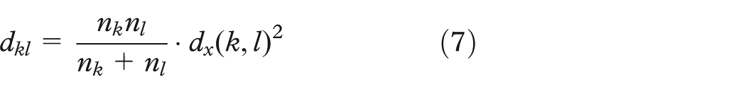
where k and l represent clusters, $n_{k}$ and $n_{l}$ represent the cardinality of clusters k and l, and $‖ c_{k} - c_{l} ‖^{2}$ represents the squared Euclidean distance between the cluster centers of clusters k and l. When clusters k and l are merged to cluster h, the cardinality $n_{h}$ is the sum of $n_{k}$ and $n_{l}$ and the centroid $c_{h}$ is the mean of $c_{k}$ and $c_{l}$ weighted by $n_{k}$ and $n_{l}$ . Hence, this specification accounts for cluster size. A particularly advantageous feature of hierarchical methods is that agglomeration can be restricted to some specific property of the underlying similarity relations between clusters. For instance, the distance between nonadjacent clusters can be set to infinite, where adjacency needs to be defined. Again, clusters can be said to agglomerate as to minimize the Euclidean distance to the centroids or the squared error function.

DDR combinations for the task at hand

Reducing dimensionality may be motivated by a large number of reasons. With no detailed treatment of how to preserve structures, and what are the similarity relations of crucial interest in various tasks, we can categorize dimension reductions by relating them to three broad aims: (1) visualization and exploration, (2) regression, and (3) classification. This boils down to the following question: What are the tasks that the methods perform and the functionalities that are needed? Lee and Verleysen⁶ describe the key functionalities of dimension reductions as follows: (1) to estimate the number of latent variables, (2) to reduce dimensionality by embedding data, and/or (3) to recover latent variables by embedding data. The task in this article, and the focus hereafter, relates to embedding data into a lower dimension to support data compression and visualization.

This section provides a detailed presentation of specific aims, needs, and restrictions of DDR combinations for visual financial performance analysis. From this discussion, we pinpoint criteria of DDR combinations relevant for capturing the suitability of methods for the task at hand.

Aims and needs for the task

The aim of models for visual financial performance analysis is to represent high-dimensional and large-volume data of financial entities in easily understandable formats. Data and dimension reductions hold promise for the task, but the aim of the models still set some specific needs and restrictions. While recent advances in information technology have enabled access to databases with nearly endless amounts of financial information (e.g. Bankscope, Bloomberg, Standard & Poor’s Capital IQ), financial data are oftentimes problematic in being incomplete and non-normal.² For instance, in the case of representing a financial entity with its balance-sheet information, it is more common than not that some items of the balance sheet are missing. Since Deakin’s² early tests of normality, where most ratios were shown to have a positive skew, the literature has been unanimous about non-normality, with explanations like lower limits of zero and parallels ranging from power-law distributions to Benford’s law. While there exist a multitude of preprocessing methods for transforming, normalizing, and trimming data, the tails of financial ratio distributions are oftentimes of high interest. This derives two necessities: the computational cost of the method needs to be considerably low and scalable, and the method needs to be flexible for problematic data.

The main aim of the low-dimensional mappings, which for this task are 2D, is to use them as displays for additional visualizations, in particular for (1) individual data, (2) structural properties of data, and (3) qualities of the models. This is due to three respective reasons: (1) the 2D plane should function as a basis or display for visual performance comparisons of financial institutions (i.e. individual data); (2) for the human brain to recognize patterns in data, we need to provide guidance for interpreting general data structures and oftentimes possess other linkable information as well; and (3) qualities of a dimension reduction may vary across mappings and locations in mappings as all information cannot be correctly preserved in a lower dimension.

The rationale behind using dimension reduction methods to create such a display is that it provides a basis on top of which individual high-dimensional data can be positioned. Moreover, given an understanding of the properties of the reduced space, which is supported by linking additional information to the display, we can also understand what positions and movements of these individual data mean on the low-dimensional display. The main aim of these mappings is hence not to be an end, but rather to function as a starting point or basis for a wide range of visualizations.

Aims and needs of DDR combinations

When evaluating or comparing performance of data and dimension reduction methods, particularly DDR combinations, quantitative measures have difficulties in accounting for qualitative differences in properties of methods. Hence, we translate the above-discussed needs for visual financial performance analysis into four qualitative criteria for evaluating DDR combinations: form of structure preservation, computational cost, flexibility for problematic data, and shape of the output.

Form of structure preservation

As stressed above, all relations in a high-dimensional space cannot be correctly preserved in a lower dimension. Hence, methods differ in what locations are stressed when preserving the structure. Given these differences, the main characteristics of structure preservation should obviously match important desires of the particular task at hand. The key question is thus “Which relations are of central importance for visual financial performance analysis?” One key aim of a dimension reduction for financial performance analysis is to create a basis or display on top of which individual data are visualized. Hence, with a main focus on visualizing individual financial entities on a low-dimensional display, correctly locating neighboring financial institutions becomes particularly important. This leads to trustworthiness of neighborhood relationships being more important than precision on the exact distance to those far away. Noise and erroneous data as well as comparability issues related to reporting differences, for instance, also motivate aiming at a mapping with local orderliness rather than focusing on global detail.

Computational cost

We oftentimes have access to vast amounts of financial data in today’s databases, including high-dimensional data for a large number of entities with a high frequency over long periods. For instance, if the used data are based upon market sources (e.g. credit default swap (CDS) spreads, equity prices, bond yields), one is easily drowned in data. This obviously sets some restrictions on computational cost and scalability of methods. While we acknowledge that computation time is not entirely a qualitative property, it has still not been incorporated in quantified evaluation measures. As noted in Van der Maaten et al.,⁶⁴ the practical applicability of a dimension reduction method relies upon its computational complexity, as application becomes infeasible if the computational resources needed are too large. In addition to the properties of data, computational cost of a method is set by the dimensionality of the output, the definition of a neighborhood in the case of neighborhood preservation, and for iterative techniques, the number of iterations, not to mention the form of input data (e.g. pairwise distance matrices or high-dimensional data points). It is also worth to consider that computational expense is a one-off cost not only when creating a dimension reduction but also when updating it. Combinations with data reduction methods may also affect the computational cost of a dimension reduction. We acknowledge that a cutoff between computationally costly and non-costly methods is difficult. Yet, the differences between methods, in particular among first-generation methods, tend to be significant.

Flexibility for problematic data

Methods differ in flexibility for non-normal and incomplete data, something more common than not in real-world financial settings. Hence, desired properties of dimension reduction methods are flexibility for incomplete and non-normal data. While the former can be defined in terms of treatment of missing values, the latter depends largely on the task at hand. Most often data are preprocessed for ideal results, including treatment of skewed distributions. Yet, preprocessing seldom does, and is most often not desired to, compress the data into uniform density. Oftentimes, the most extreme values of financial ratios are among the most interesting states of financial performance. Hence, one type of tolerance toward outliers can be derived from the output of methods. A method is assessed to be tolerant toward outliers and skewed distributions if problematic data do not impair the intelligibility of an output or display (e.g. stretch toward outliers).

Shape of the output

One of the main aims is to use a dimension reduction as a display to which we link additional visualizations. In particular, we use the low-dimensional mappings as displays for information such as individual data and structural properties. This turns the focus to the shape of the outputs or mappings. Outputs of dimension reduction mappings can take a wide range of forms. We consider the interrelated properties of the shape to be continuous versus discrete mappings, optional versus mandatory data reductions, and predefined versus data-driven grid shapes. While a mandatory data reduction is generally not desirable, we do not consider it a direct disadvantage, rather the opposite, due to the large amounts of available data. This leads also to restricting mappings to discrete rather than continuous, whereas continuous mappings would obviously be desirable for precision. The largest difference for interpretation, especially in terms of linking visualizations, is between predefined and data-driven grid shapes. This also implies mandatory data reduction and discrete mappings. While methods with data-driven grid shapes may better adapt to data, the methods with predefined grid shapes are superior in functioning as a regularly formed display for additional visualizations, not the least when linking information to the produced display (or units of it). This is a key property as the mappings are starting points rather than ending points of the analysis, where additional visualizations may comprise individual data, structural properties of data, and qualities of the models.

Qualitative and quantitative experiments

This section introduces data and dimension reductions to financial performance analysis. We first discuss the relative goodness of methods for the task from a qualitative perspective. Then, we illustrate how data and dimension reduction methods can be utilized for visual financial performance analysis of European banks.

For dimension reduction, we consider the SOM, metric MDS, and Sammon’s mapping. Metric MDS and Sammon’s mapping belong to the group of distance-preserving methods, while the SOM belongs to the group of topology-preserving methods with a predefined grid shape. For data reduction, we consider Ward’s hierarchical clustering, k-means clustering, and VQ. Due to access to overabundant amounts of financial data, we concentrate herein mainly on serial and parallel combinations of these stand-alone methods for DDR combinations. While the SOM performs DDR by default, large SOMs can be further enhanced by a second-level clustering of its prototypes. Conceptually, the functioning of the SOM differs from the other DDR combinations as the two tasks of data and dimension reduction are treated as concurrent subtasks. In serial combinations, the dimension reduction is always subordinate to the data reduction, while parallel combinations deal separately with the initial dataset.

A qualitative comparison

This section presents a qualitative discussion of DDR combinations for visual performance analysis and relates it to the four identified criteria: form of structure preservation, computational cost, flexibility for problematic data, and shape of the output.

Form of structure preservation

The main difference between DDR combinations is how the dimension reduction methods differ in the properties of data they attempt to preserve. For our task, this leads to one key question: Which methods better assure trustworthy neighbors? MDS-based methods with objective functions attempting distance preservation, while likely being better at approximating distance structures, may end up with skewed errors across the projection. While metric MDS weights distances equally, Sammon’s mapping turns its focus to local distance, but still aims at preserving interpoint distances. Yet, it has been shown that the SOM, which stresses neighborhood relations, better assures trustworthy neighbors.^10,51 That is, data found close-by each other on the SOM display are more likely to be similar in terms of the original data space, and similar data in the original space are also more likely to be found close-by on the SOM. The conceptual difference in structure preservation between distance- and topology-preserving methods is illustratively described by Kaski with an experiment on a curved 2D surface in a three-dimensional space: the former methods may follow the surface in data with two dimensions, whereas the latter require three dimensions to describe the structure. Likewise, in a financial setting, the SOM assures that the set of banks under analysis are located in a ranking-order manner on the low-dimensional display such that close-by banks are also likely to be similar in the high-dimensional space.

Computational cost

Expensive computation is obviously an issue when dealing with large financial datasets. Generally, computing pairwise distances between data is costly and the order of magnitude is N², which clearly relates to the distance preservation of both metric MDS and Sammon’s mapping. The topology preservation of the SOM relates instead to the grid size M with an order of magnitude of M².⁶⁶ This implies that the complexities of the methods are similar if the grid size M equals the number of data N, but more importantly that the SOM allows for adjusting M for cheaper complexity. Furthermore, parallel DDR combinations suffer from an additional computational cost as the clustering is performed on the initial dataset rather than on a reduced number of prototypes. The computational cost of MDS-based methods motivates serial DDR combinations. Another issue related to computational cost is the lack of an explicit mapping function for the MDS-based methods. Hence, when including new samples, the projection needs to be recomputed. While new samples can be visualized via projection to their best-matching data, each update requires recomputing the projection. (While relative MDS⁶⁷ allows to add new data to the basis of an old MDS, it does still not update all distances within the mapping.) In contrast, the SOM can be cheaply updated with individual data using a sequential algorithm.

Flexibility for problematic data

The methods differ in flexibility for problematic data. Methods dealing with distance preservation, including both metric MDS and Sammon’s mapping, have difficulties with incomplete data in that they have their basis in a distance matrix. However, the SOM, and its self-organization, can be seen as tolerant to missing values by only considering the available ones in matching.⁶⁸ In practice, the SOM has been shown to be robust when up to approximately one-third of the variables are missing.^58,68–70 Indeed, the SOM has even been shown to be effective for imputing missing values.⁷² Tolerance toward outliers is defined in terms of representation of skewed distributions. An MDS-based mapping becomes difficult to interpret if it is stretched toward directions of outliers and extreme tails. While the processing of the SOM does not per se treat outliers, its regularly shaped grid of prototypes facilitates visualizing data with nonuniform density functions.

Shape of the output

A key to using a dimension reduction as a display, and linking information to it, is the shape of its output. While the SOM has a discrete mapping, mandatory data reduction, and predefined grid shape, MDS-based methods, including metric MDS and Sammon’s mapping, are its contrasts by having continuous mappings, optional data reduction, and data-driven lattice (if combined with data reduction). The predefined SOM grid, while also having drawbacks for representing structural properties of data, facilitates the interpretation of linked information. Today, it is standard that the SOM comes with a wide set of linked extensions for visual analytics, such as the so-called component planes, U-matrix, and frequency plots (see, for example, Vesanto⁷³). Even though visual aids for showing distance structure and density compensate for constraints set by the grid shape, there is a large group of other aids that enhance the representation of available information in data. The visual aids, while not always being even applicable, have generally not been explored in the context of MDS-based projections. Component planes, for instance, are difficult to visualize due to the lack of a reduced number of prototypes. Even DDR combinations with serial VQ, that is, processing similar to that of the SOM, would still lack the concept of neighborhood relations of a regularly shaped grid.

Illustrative experiments

The qualitative discussion of properties of DDR combinations for financial performance analysis still lacks illustrations of the above-discussed properties of methods. Here, we show some illustrative experiments with the previously discussed methods. Dimension reduction is performed with the SOM, metric MDS, and Sammon’s mapping and data reduction with Ward’s hierarchical clustering, k-means clustering, and VQ. We explore various combinations of DDR for achieving easily interpretable models for visual financial performance analysis. The methods are chosen and combined as per their suitability for data reduction of dimension reductions and vice versa.

Data

The dataset used in this article consists of annual financial ratios for banks from the European Union, including all provided financial ratios in the Bankscope database from Bureau van Dijk. Generally, financial data may have a wide range of challenging properties, which should mostly be addressed differently depending on the task at hand. The preprocessing in this article is performed with respect to the task defined in section “DDR combinations for the task at hand.” As the aim is to have a dataset for illustrative experiments, and a more complex preprocessing of data would neither alter the results of a qualitative nor a quantitative comparison, the preprocessing and its discussion are also kept fairly simple.

Initially, the dataset consisted of 38 annual financial ratios for 1236 banks spanning from 1992:12 to 2008:12. A large concern in the dataset is the share of missing values. We chose to use 24 ratios by dropping those with more than 25% missing data. Observations with missing values for more than one-third of the ratios were removed. Finally, we were left with a resulting 9655 rows of data and a total of 855 banks. Yet, the dataset still includes missing values.

Although the SOM is tolerant to missing data, we need to impute them in this work as distance-preserving methods require complete data. We use the SOM for imputing missing values, as it was found to be more accurate than other common, simple methods. Moreover, it has been commonly used for imputing missing values in the literature (see, for example, Cottrell and Letrémy⁷³), and this circumvents the introduction of a new method. The SOM allows mapping incomplete data to their BMUs by only considering the available variables. Hence, complete data were used for training the SOM, incomplete data were mapped to their BMUs, and the missing values were imputed from their BMUs.

In addition to the SOM, we test three other techniques: the value of the previous year (t− 1) and the mean and median of each variable. The performance of the methods was compared by imputing randomly generated missing values in 10% of the complete data. The methods were evaluated in terms of the root mean square deviation (RMSD) of the imputed values from the real ones. The SOM was found to be most accurate when the grid size was smaller than 20 units. The optimal, and chosen, grid size was 3 × 3.

Moreover, although outliers are not a problem per se, they still affect the interpretability of the models, not the least MDS-based approaches. Not to lose significant amounts of data, we use modified boxplots for trimming with replacement, resulting in replacing data as needed per variable and tail.

We have used the entire dataset in each of the experiments in this article, in particular when creating displays with data and dimension reduction methods. Still, we depart from the entire dataset in two manners. First, data reductions and VQs of the data may from time to time function as inputs in subsequent steps. Second, illustrative cases from the overall dataset are used as sample trajectories for visualizing individual data on the created displays. The trajectories consist of all input variables spanning from 2002 to 2008 for Deutsche Bank, ABN AMRO, and Société Général.

Parallel DDR

Figure 2 shows parallel DDR combinations on the entire dataset. Sammon’s mapping is combined with k-means clustering, and MDS and the SOM are combined with Ward’s clustering. In parallel DDR combinations, we first apply the dimension reduction methods (MDS, Sammon’s mapping, and the SOM) on the entire dataset and cluster the data for MDS and Sammon’s mapping and the units for the SOM using data reduction methods (Ward’s and k-means clustering). When training SOMs, one has to set a number of parameters. To parameterize the SOM, we use a set of quality measures to track the topographic and quantization accuracy as well as clustering of the map. The map format is chosen to be 75:100, as it approximates the recommended ratio of the two largest eigenvalues (see, for example, Kohonen⁵⁹). The objective functions of MDS-based methods are optimized with an iterative steepest-descent process. Ward’s clustering of the SOM is, however, performed on its prototypes rather than on the dataset and restricted to agglomerate only adjacent clusters in the SOM topology. We do not, however, consider this option for MDS-based projections as there is no natural definition of adjacency. On top of all three mappings, we superimpose cluster color coding and a performance comparison of trajectories from 2002 to 2008 for three large European banks. The projections of MDS and Sammon’s mapping on this large dataset are very similar, whereas k-means clustering has less overlapping cluster memberships in the mapping than Ward’s clustering. The trajectories as well as the underlying variables confirm that while the orientations of the two MDS-based projections are different from those of the SOM model, their structure is still very similar. Yet, the computational cost differs remarkably. While it takes on an ordinary personal computer only a few seconds to train SOM-based models on these data, the MDS-based projections require several hours on a dedicated server.

Figure 2.

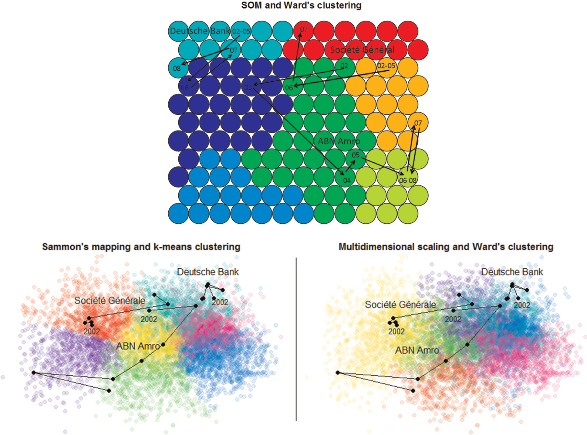
Parallel DDR combinations applied to the financial dataset, as well as trajectories for three large European banks from 2002 to 2008.

Serial DDR

For cheaper complexity, we further explore possibilities of DDR by testing serial combinations. In serial DDR combinations, we first apply the data reduction methods (Ward’s and k-means clustering) on the entire dataset and then project the cluster centroids of k-means and second-level clustering of the SOM using dimension reduction methods (Sammon’s mapping). Figure 3 shows Sammon’s mapping of the k-means cluster centroids as well as the second-level centroids of the SOM, where size represents the number of data in each cluster. This type of usage of MDS-based methods was already proposed by Sammon¹⁵ due to their high computational cost and later applied by Flexer,⁹ for instance. It is, indeed, a cheap way to illustrate relations between the cluster centroids but lacks details for structural as well as individual analysis. Hence, while being cheap, none of these two serial approaches support the task at hand.

Figure 3.

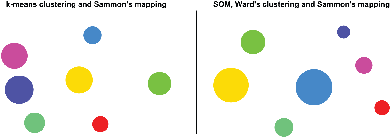
Serial DDR combinations applied to the financial dataset.

Serial and parallel DDR

Costly but detailed MDS-based projections in Figure 2 and cheap but crude projections in Figure 3 motivate finding a compromise solution. For reducing computational expense, we still end up relying on a serial DDR combination. For more details, however, we attempt to reduce the initial dataset to a smaller but representative dataset. This type of data compression can be achieved with standard VQ that approximates probability density functions of data. The compressed prototypes can then be used as an input for a parallel DDR. In serial and parallel DDR combinations, we first reduce the entire dataset into fewer prototypes with VQ methods (standard VQ and the SOM) and then project the prototypes using a dimension reduction (Sammon’s mapping). Thereafter, we reduce the number of prototypes using k-means and Ward’s clustering and superimpose the cluster memberships on top of the mappings through color coding. Conceptually, while still lacking the interaction between the tasks as well as the regular grid shape, we come close to what is achieved using the SOM in Figure 2 by relying on both serial and parallel DDR combinations. The left plot in Figure 4 shows a VQ of the initial dataset and then a subsequent Sammon’s mapping and k-means clustering on the VQ prototypes. To illustrate the difference between the SOM- and MDS-based approaches, the right plot in Figure 4 shows a corresponding Sammon’s mapping of SOM prototypes with a superimposed cluster color coding. This figure shows two issues: the ordered SOM prototypes have less overlap of cluster memberships and the importance of naturally defined topological relations. The former issue is most likely a result of interaction between the tasks of data and dimension reduction but might also benefit from the inclusion of neighborhood relations when agglomerating clusters. The latter issue of a regularly shaped grid is particularly useful when attempting to visualize as much of the available information as possible through linked visualizations.

Figure 4.

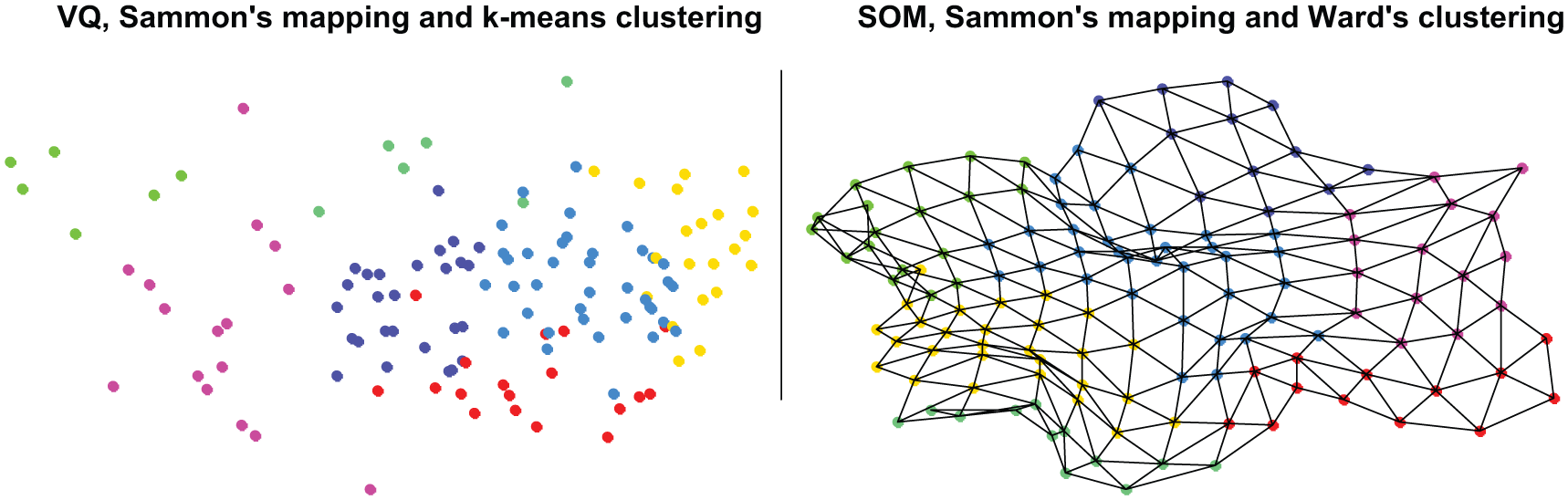
Serial and parallel DDR combinations applied to the financial dataset.

The SOM and its visualization aids

This section first briefly reviews visualization aids for the SOM and then illustrates the use of the regularly shaped SOM grid and its visualization aids. Figure 2 showed the 2D SOM grid and trajectories for three large European banks from 2002 to 2008, but a central question remains: How should we interpret the map? The possibility of linking additional information to the SOM grid has stimulated the development of a wide scope of visualization aids (see Vesanto⁷³ for an early overview). Generally, the aids fall into one of the following three groups: (1) those compensating structural properties inherent in data that the regular grid shape eliminates, (2) those extending the visualization of properties inherent in data but not normally accessible in dimension reductions, and (3) those linking the SOM grid with other methods or data to enhance the understanding of the task.

The first group includes means to represent the distance structure and density on an SOM, something missing due to the VQ and grid shape. Densities on the SOM are generally assessed with frequency plots and the Pareto density estimation matrix (P-matrix).⁷⁴ Examples of aids for assessing distance structures are Sammon’s mapping, the Unified distance matrix (U-matrix),⁷⁵ and cluster connections.⁷⁶ Moreover, some methods attempt to account for both structures and densities, such as the U*-matrix,⁷⁷ the sky metaphor visualization,⁷⁸ the neighborhood graph,⁷⁹ and smoothed data histograms.⁸⁰

The second group consists of visualizations that enhance the representation of multidimensional information. Component planes are a standard method for visualizing the spread of values of individual dimensions on the SOM, but they have been further enhanced in several aspects. For instance, Vesanto and Ahola⁸¹ use an SOM for reorganizing the component planes according to correlations, and Neumayer et al.⁸² introduced the metro map discretization to summarize all component planes onto one plane. Kaski et al.⁸³ have developed a visualization of the contribution of each variable to distances between prototypes, that is, the cluster structure. Another extension, while partly also belonging to the other groups, is visualization of vector fields⁸⁴ for assessing contributions to the cluster structure and for finding correlations and dependencies in the underlying data.

The third group uses other methods or data for further enhancing the understanding of the task. One common way to represent cluster structures in an SOM is applying a second-level clustering on the prototypes and visualizing it through color coding.⁸⁵ This has also been done using fuzzy methods,²⁸ where soft memberships of prototypes in each cluster can be represented on their own grids or associated with individual data. The strengths and directions of state transition patterns on an SOM can similarly be represented on own grids, such as prototype-to-cluster transition probabilities in Sarlin et al.,⁸⁶ not to mention using the prototypes as an input for some other predictive methods, such as the neural network in Serrano-Cinca (1996),⁸⁷ and visualizing the prediction on the SOM grid. An example of combining the display of an SOM with other data is to link network relations between entities on the grid.⁸⁸ In a financial setting, this enables relating the state of financial performance of a cross section of entities to their network relations, that is, systemic relevance.

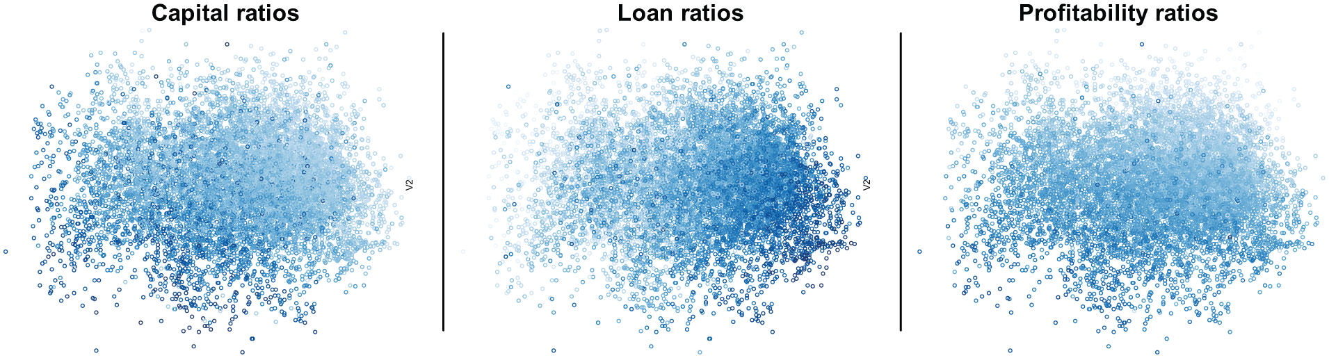
Here, we show some examples of how visualizations from the above three groups can be linked to the SOM. Figure 2 already showed a financial performance comparison over time of three large European banks using labels and trajectories. Figure 5 uses the regular shape of the SOM grid as a basis for nine different representations of additional information. The spread of values on the SOM is shown using a Color Brewer’s scale,⁸⁹ where variation of a blue hue occurs in luminance (light to dark represent low to high values). First, Figure 5(a)–(c) illustrates structural properties of the model: Figure 5(a) shows hard cluster memberships of the second-level clustering, Figure 5(b) shows distance structures using a U-matrix visualization, and Figure 5(c) shows the frequency distribution on the SOM grid. While Figure 5(a) and (b) shows similar characteristics of cluster structures, where the latter is more detailed, Figure 5(c) shows that the lower-right corner of the map is comparatively more dense. Second, Figure 5(d)–(f) enables assessing correlations and distributions by showing the spread of three financial performance measures on the SOM grid: capital, loan, and profitability ratios. Here, one can observe that, generally, the right part represents well-performing and the left part poor banks. Third, Figure 5(g)–(i) illustrates temporal transition patterns by showing for each prototype the probability of transition to three areas on the SOM grid: Clusters A, B, and C (good); Cluster D (average); and Clusters E, F, and G (poor banks). The figure shows that while the left part (poor) is more stable than the right (good), the center is a transition cluster. Hence, the first group is represented by Figure 5(b) and (c); the second group by Figure 5(d)–(f); and the third group by Figure 5(a), (g), (h), and (i). Given the additional information of the SOM display in Figure 5, we can revisit Figure 2 for a better understanding of the time-series visualizations of individual banks. For instance, the trajectory of ABN AMRO confirms that the performance of the bank itself, while being involved in a takeover by Royal Bank of Scotland and Fortis and their subsequent failures, has been improving over the years.

Figure 5.

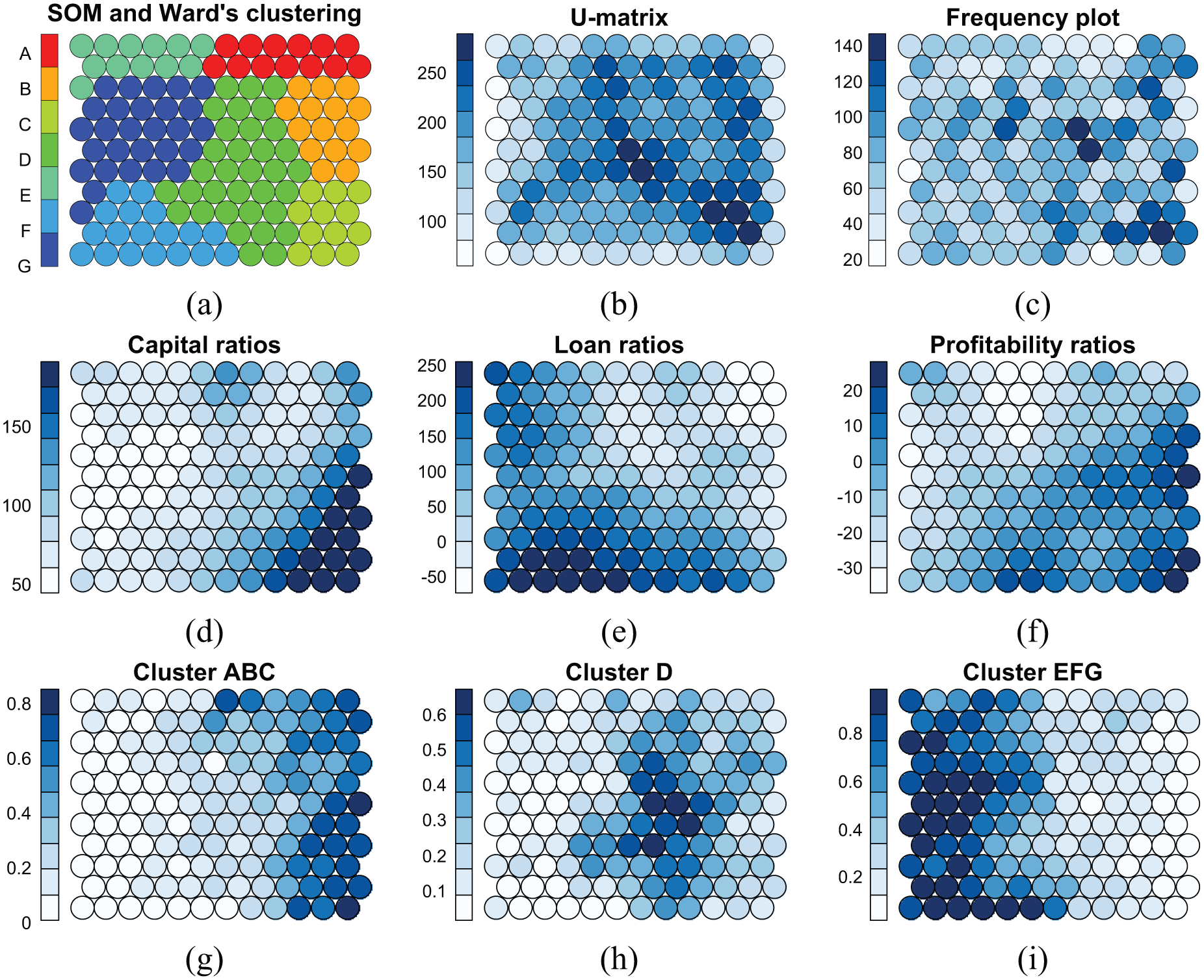
An exemplification of linking information to the SOM grid. Charts (a)–(c) illustrate structural properties of the model: (a) cluster structures by showing cluster memberships of the second-level clustering, (b) more detailed structures by showing average distances between prototypes or the so-called U-matrix, and (c) the density on the SOM grid by showing frequencies per SOM unit. Charts (d)–(f) represent univariate information of the multivariate SOM by showing the spread of three individual variables measuring financial performance on the SOM grid: capital, loan, and profitability ratios. Charts (g)–(i) represent the temporal structure of the grid by showing for each unit the probability of transition to three areas on the SOM grid: Clusters A, B, and C; Cluster D; and Clusters E, F, and G.

Yet, a central question remains: What is the potential of using visualization aids in combination with MDS-based mappings? Although we noted above that the regularly shaped and predefined SOM grid facilitates linking information, MDS-based mappings can also be linked with additional information. Yet, the so-called hairball visualizations of complex networks, where nodes and edges are so large in number that they challenge the resolution of computer displays, not to mention interpretation, also relate to the view of MDS-based mappings. Likewise, a large share of processing is left for the human visual system to perform, as the number of data has not been decreased. However, given that one would approach a task for which an MDS-based mapping holds most promise, there is still added value in combinations with visualization aids. For instance, Figure 6 exemplifies how “component planes” for Sammon’s mapping visualize the spread of individual variables over Sammon’s mapping coordinates.

Figure 6.

An exemplification of linking information to Sammon’s mapping.

Discussion

This article has considered data and dimension reduction methods, as well as their combination, for visual financial performance analysis. The discussions and illustrations in section “Qualitative and quantitative experiments,” while being at times somewhat trivial, are motivated by inconsistency of argumentation for and application of various methods. The main conclusion of the comparison is that the SOM has several useful properties for financial performance analysis. In particular, we have noted the following advantages of the SOM over alternative distance-preserving methods: (1) trustworthy neighbors, (2) low computational cost, (3) flexibility for problematic data, and (4) a regularly shaped grid. It is, however, worth noting that the relative goodness of a method depends always on the task in question. That said, the SOM is obviously far from a panacea for all sorts of data and dimension reduction. When only attempting stand-alone tasks, it is indeed very likely that there exist better methods than the SOM. Similarly, when attempting DDR, the superiority of one method over others depends entirely on the aims of the task in question.

Even though the SOM has been assessed as superior for visual financial performance analysis, it is worth to carefully consider its limitations:

The SOM performs a crude mapping. Rather than data points, the SOM attempts to embed the prototypes. A significant constraint if detail is of central importance and if only projecting a few data points.

The regular grid shape sets some restrictions on the SOM. For instance, it may cause interpolating sparse locations with idle prototypes, lead to an end user overinterpreting the regular-like y- and x-axes, and lead to the need for additional visual aids to fully represent structures.

Mathematical treatment of the SOM has shown to be problematic. The lack of an objective function, as well as a general training schedule for or proof of convergence, complicates assessing convergence of an SOM.

The comparison in this article has covered classical first-generation dimension reduction methods. The main question that still remains is “Can the results of this comparison be generalized to all available methods?” As reviewed in section “Related literature,” CCA has been shown to outperform the SOM in terms of trustworthiness of neighborhood relations.^52,53 Likewise, two more recent local versions of MDS, denoted as LMDS, by Venna and Kaski³⁹ and Chen and Buja⁴⁰ adapt the functioning of standard MDS to preserve local relations. These methods, while holding promise for one criterion, fall short in other, not the least in the shape of the output. It is thus important to consider methods from the second generation with the key properties of the SOM. To the best of our knowledge, there are two conceptually similar topology-preserving methods that possess DDR capabilities and a predefined grid shape: GTM and XOM. GTM mainly differs from the SOM by relying on well-founded statistical properties based upon Bayesian learning with an objective function, namely, the log-likelihood, which is optimized by the expectation–maximization algorithm. This objective function directly facilitates assessing convergence of the GTM. Even though Bishop et al.⁹⁰ originally stated that the GTM is computationally comparable to the SOM, it has later been shown that the SOM is cheaper.⁹¹ This may result from the number of developed algorithmic shortcuts for computing SOMs, such as fast-winner search.⁹² Both methods are flexible for problematic data, that is, outliers and missing values, through a similar predefined grid shape and an extension of the GTM for treating missing values.^92,93 However, while choosing parameters for the SOM may be a tedious task, given adequate initializations and parameterizations, convergence has seldom appeared to be a problem in practice.⁶² A decade after the introduction of the GTM, neither it nor its variants, such as the S-Map, have displaced the standard SOM.

The XOM is a computational framework for data and dimension reduction. By inverting the functioning of the SOM, the XOM systematically exchanges functional and structural components of topology-preserving mappings by self-organized model adaptation to the input data. It has two main advantages compared to the SOM: (1) reduced computational cost and (2) applicability to nonmetric data as there is no restriction on the distance measures. Even though the use of nonmetric dissimilarity measures is of little use on the data in this article, while still having potential for other pairwise financial data, the reduced computational cost is particularly beneficial for large financial datasets in general. The XOM has, however, been recently introduced and is thus still lacking thorough tests in relation to other methods, such as comparisons to SOMs with algorithmic shortcuts. Yet, the XOM should be considered as a valid alternative to the SOM paradigm.

The above discussion is summarized in Table 1, where methods fulfilling the criteria are shown. CCA and LMDS are only shown as examples of second-generation methods that partially fulfill the criteria. The key message is thus that all four criteria are fulfilled by three methods that perform a topology-preserving mapping to a regularly shaped grid: the SOM, GTM, and XOM. It is worth to note, as widely suggested,^6,13 that one of the main reasons for the SOM being very popular for a broad range of tasks, such as classification, clustering, visualization, prediction, and missing value imputation, might be because it produces an intuitive output using a simple and an intuitive formulation. This simplicity, while being beneficial for a method to be widely accepted, applied, and understood, still should not be used for assessing relative goodness. One should, nevertheless, note that when introducing dimension reductions to the general public, such as policy- or decision-makers in general, simplicity is definitely an asset. To this end, this article argues that the optimal method for financial performance analysis is one from the family of methods that perform a topology-preserving mapping to a regularly shaped and predefined grid.

Table 1.

A summary of the qualitative and quantitative comparisons of DDR methods, including a projection into second-generation methods.

	Form of structure preservation	Computational cost	Flexibility for problematic data	Shape of the output
First generation	SOM	SOM, MDS,^a Sammon’s^a	SOM	SOM
Second generation	CCA, LMDS, GTM, XOM	CCA, GTM, XOM	GTM, XOM	GTM, XOM

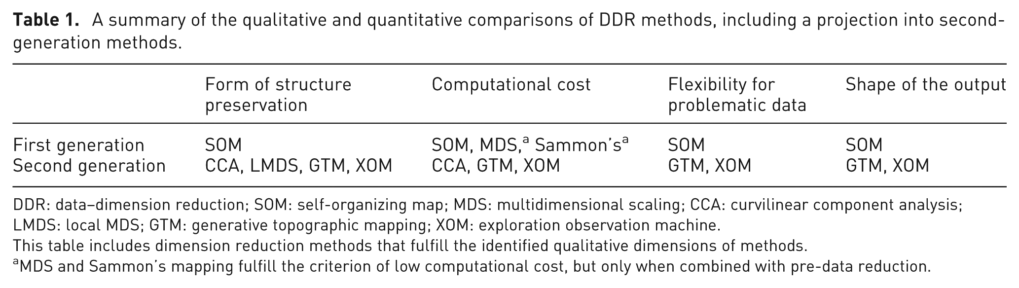
DDR: data–dimension reduction; SOM: self-organizing map; MDS: multidimensional scaling; CCA: curvilinear component analysis; LMDS: local MDS; GTM: generative topographic mapping; XOM: exploration observation machine.

This table includes dimension reduction methods that fulfill the identified qualitative dimensions of methods.

MDS and Sammon’s mapping fulfill the criterion of low computational cost, but only when combined with pre-data reduction.

Conclusion

Every task has its own needs. Data and dimension reduction for the task of visual financial performance analysis should thus be performed with methods that have the best overall suitability for that task, not the best processing capabilities for some other objective. The overall task discussed in this article is to represent high-dimensional data concerning financial entities on low-dimensional displays, to which additional visualizations can be linked, such as (1) individual data, (2) structural properties of data, and (3) qualities of the models. To this end, this article has addressed the choice of method for visual financial performance analysis from a qualitative perspective. We have first discussed the properties of three inherently different classical first-generation dimension reduction methods, and their combination with data reduction, and illustrated their performance in a real-world financial application. The conclusion drawn from the comparison of classical methods was then prolonged to second-generation methods. The qualitative discussion and experiments showed superiority of the SOM for financial performance analysis in terms of four criteria: form of structure preservation, computational cost, flexibility for problematic data, and shape of the output. When considering second-generation methods, the recently introduced GTM and XOM have clear potential for similar tasks. GTM improves the SOM paradigm with its well-defined objective function, but is computationally more costly, while XOM is a recently introduced promising method, but still lacks thorough comparisons.

From the discussions in this article, an obvious conclusion is that the family of methods that perform a topology-preserving mapping to a regularly shaped and predefined grid provides means for visual financial performance analysis. The aims and needs for the task at hand, where the main focus lies on using the output as a display for additional information in general and individual data in particular, are neither rare objectives in other fields. While not being generalizable to their full extent, parts of the conclusions herein will also apply in other fields and domains. The methods advocated in this article do not, however, provide a panacea for visual financial performance analysis. They should be paired with other methods, not least visualizations of different kinds, that compensate for missing properties when having, for instance, a regularly shaped grid. It also motivates exploring the information commonly linked to the SOM in not only the same family of methods with predefined grid shapes but also other dimension reduction paradigms in general. In addition, while the family of methods that perform a topology-preserving mapping to a predefined grid exhibits favorable properties for the task at hand, we pointed out a lack of comparisons of these methods. Future work should hence focus on comparing the SOM, GTM, and XOM not only for the task at hand but also for the common aim of the methods, allowing for assessing the superiority of one dimension reduction method over others with a quantitative measure.

Footnotes

Acknowledgements

The author wants to thank Barbro Back and Tomas Eklund, and seminar participants at the Data Mining and Knowledge Management Laboratory on 13 February 2012, IS Seminar at Åbo Akademi University on 1 March 2012 and Bank of Finland Financial Stability Seminar on 11 November 2011 for useful comments.

Funding

This research received no specific grant from any funding agency in the public, commercial, or not-for-profit sectors.

References

Nobes

. The survival of international differences under IFRS: towards a research agenda. Account Bus Res 2006; 36(3): 233–245.

Deakin

. Distributions of financial accounting ratios: some empirical evidence. Account Rev 1976; 51: 90–96.

Zopounidis

Despotis

Stavropoulou

. Multiattribute evaluation of Greek banking performance. Appl Stoch Model D A 1995; 11: 97–107.

Demyanyk

Hasan

. Financial crises and bank failures: a review of prediction methods. Omega 2010; 38(5): 315–324.

Halkos

Salamouris

. Efficiency measurement of the Greek commercial banks with the use of financial ratios: a data envelopment analysis approach. Manage Account Res 2004; 15: 201–224.

Lee

Verleysen

. Nonlinear dimensionality reduction. Berlin: Springer, 2007.

Kohonen

. Self-organized formation of topologically correct feature maps. Biol Cybern 1982; 66: 59–69.

Flexer

. Limitations of self-organizing maps for vector quantization and multidimensional scaling. In: Mozer

Jordan

Petsche

(eds) Advances in neural information processing systems 9. Cambridge, MA: MIT Press, 1997, pp. 445–451.

Flexer

. On the use of self-organizing maps for clustering and visualization. Intell Data Anal 2001; 5(5): 373–384.

10.

Venna

Kaski

. Neighborhood preservation in nonlinear projection methods: an experimental study. In: Proceedings of the international conference on artificial neural networks (ICANN’01), Vienna, 21–25 August 2001, pp. 485–491. Berlin: Springer.

11.

Lee

Verleysen

. Quality assessment of dimensionality reduction: rank-based criteria. Neurocomputing 2009; 72(7–9): 1431–1443.

12.

Lueks

Mokbel

Biehl

. How to evaluate dimensionality reduction? In Proceedings of the workshop on new challenges in neural computation, Frankfurt, Germany, 30 August 2011.

13.

Trosset

. Representing clusters: k-means clustering, self-organizing maps, and multidimensional scaling. Technical Report 08–03, 20 February 2008. Bloomington, IN: Department of Statistics, Indiana University.

14.

Torgerson

. Multidimensional scaling: I. Theory and method. Psychometrika 1952; 17: 401–419.

15.

Sammon

. A non-linear mapping for data structure analysis. IEEE T Comput 1969; 18(5): 401–409.

16.

Linde

Buzo

Gray

. An algorithm for vector quantizer design. IEEE T Commun 1980; 28(1): 702–710.

17.

MacQueen

. Some methods for classification and analysis of multivariate observations. In: Proceedings of the fifth Berkeley symposium on mathematical statistics and probability (eds Le Cam

L M

Neyman

). Berkeley, CA: University of California Press, 1967, pp. 281–297.

18.

Ward

. Hierarchical grouping to optimize an objective function. J Am Stat Assoc 1963; 58: 236–244.

19.

Fraser

Phillips

Rose

. A canonical analysis of bank performance. J Financ Quant Anal 1974; 9(2): 287–295.

20.

Demirgüç-Kunt

Detragiache

. Monitoring banking sector fragility. A multivariate logit. World Bank Econ Rev 2000; 14(2): 287–307.

21.

González-Hermosillo

. Determinants of ex-ante banking system distress: a macro-micro empirical exploration of some recent episodes. IMF Working Paper No. 99/33, March 1999. Washington, DC: International Monetary Fund.

22.

Männasoo

Mayes

. Explaining bank distress in Eastern European transition economies. J Bank Financ 2009; 33(2): 244–253.

23.

Betz

Oprica

Peltonen

. Predicting distress in European banks. ECB Working Paper Series, forthcoming.

24.

Seçme

Bayrakdaroğlu

Kahraman

. Fuzzy performance evaluation in Turkish Banking Sector using Analytic Hierarchy Process and TOPSIS. Expert Syst Appl 2009; 36(9): 11699–11709.

25.

Kung

Kun-Li

. Applying grey relational analysis and grey decision-making to evaluate the relationship between company attributes and its financial performance—a case study of venture capital enterprises in Taiwan. Decis Support Syst 2007; 43(3): 842–852.

26.

Aigner

Miksch

Müller

. Visual methods for analyzing time-oriented data. IEEE T Vis Comput Gr 2008; 14(1): 47–60.

27.

Ezzamel

Mar-Molinero

. On the distributional properties of financial ratios. J Bus Finan Account 1987; 14: 463–481.

28.

Sarlin

Eklund

. Financial performance analysis of European banks using a fuzzified self-organizing map. International Journal of Knowledge-Based and Intelligent Engineering Systems 2013; 17(3): 223–234

29.

Mar-Molinero

Serrano-Cinca

. Bank failure: a multidimensional scaling approach. Eur J Financ 2001; 7(2): 165–183.

30.

Martín-del-Brío

Serrano-Cinca

. Self-organizing neural networks for the analysis and representation of data: some financial cases. Neural Comput Appl 1993; 1(3): 193–206.

31.

Back

Sere

Vanharanta

. Managing complexity in large data bases using self-organizing maps. Account Manag Inform Tech 1998; 8(4): 191–210.

32.

Sarlin

Peltonen

. Mapping the state of financial stability. Journal of International Financial Markets, Institutions & Money 2013; 26: 46–76.

33.

Pearson

. On lines and planes of closest fit to systems of points in space. Philosophical Magazine 1901; 2(6): 559–572.

34.

Young

Householder

. Discussion of a set of points in terms of their mutual distances. Psychometrika 1938; 3: 19–22.

35.

Shepard

. The analysis of proximities: multidimensional scaling with an unknown distance function. Psychometrika 1962; 27: 125–140, 219–246.

36.

Kruskal

. Multidimensional scaling by optimizing goodness of fit to a nonmetric hypothesis. Psychometrika 1964; 29: 1–27.

37.

Demartines

Hérault

. Curvilinear component analysis: a self-organizing neural network for nonlinear mapping of data sets. IEEE T Neural Networ 1997; 8: 148–154.

38.

Venna

Kaski

. Local multidimensional scaling. Neural Networks 2006; 19: 889–899.

39.

Chen

Buja

. Local multidimensional scaling for nonlinear dimension reduction, graph drawing, and proximity analysis. J Am Stat Assoc 2009; 104: 209–219.

40.

Bishop

Svensson

Williams

CKI

. GTM: the generative topographic mapping. Neural Comput 1998; 10(1): 215–234.

41.

Roweis

Saul

. Nonlinear dimensionality reduction by locally linear embedding. Science 2000; 290: 2323–2326.

42.

Tenenbaum

de Silva

Langford

. A global geometric framework for nonlinear dimensionality reduction. Science 2000; 290: 2319–2323.

43.

Belkin

Niyogi

. Laplacian eigenmaps and spectral techniques for embedding and clustering. In: Dietterich

Becker

Ghahramani

(eds) Advances in neural information processing systems 14. Cambridge, MA: MIT Press, 2001, pp. 586–691.

44.

Weinberger

Saul

. Unsupervised learning of image manifolds by semidefinite programming. Int J Comput Vision 2005; 70(1): 77–90.

45.

Van der Maaten

LJP

Hinton

. Visualizing high-dimensional data using t-SNE. J Mach Learn Res 2008; 9: 2579–2605.

46.

Wismüller

. A computational framework for nonlinear dimensionality reduction and clustering. In: Principe

Miikkulainen

(eds) Advances in self-organizing maps (Lecture Notes in Computer Science, vol. 5629). St. Augustine, Florida, USA: Springer, 2009, pp. 334–343.

47.

Dempster

Laird

Rubin

. Maximum likelihood from incomplete data via the EM algorithm. J Roy Stat Soc B Met 1977; 39(1): 1–38.

48.

Ester

Kriegel

H-P

Sander

. A density-based algorithm for discovering clusters in large spatial databases with noise. In: Simoudis

Han

Fayyad

(eds) Proceedings of the second international conference on knowledge discovery and data mining (KDD-96), Portland, Oregon, USA. AAAI Press, 1996, pp. 226–231.

49.

Duch

Naud

. Multidimensional scaling and Kohonen’s self-organizing maps. In: Proceedings of the 2nd conference on neural networks and their applications, Szczyrk, April 1996, pp. 138–143.

50.

Bezdek

Pal

. An index of topological preservation for feature extraction. Pattern Recogn 1995; 28: 381–391.

51.

Nikkilä

Törönen

Kaski

. Analysis and visualization of gene expression data using self-organizing maps. Neural Networks 2002; 15(8–9): 953–966.

52.

Himberg

. From insights to innovations: data mining, visualization, and user interfaces. PhD Thesis, Helsinki University of Technology, Espoo, 2004.

53.

Venna

Kaski

. Comparison of visualization methods for an atlas of gene expression data sets. Inform Visual 2007; 6(2): 139–154.

54.

De Vel

Lee

Coomans

. Comparative performance analysis of non-linear dimensionality reduction methods. In: Fischer

Lenz

H-J

(eds) Learning from data: artificial intelligence and statistics V. New York: Springer, 1996, pp. 320–345.

55.

Bação

Sousa Lobo

Painho

. Self-organizing maps as substitutes for K-means clustering. In: Proceedings of the international conference on computational science, Atlanta, GA, 22–25 May 2005, pp. 476–483. Springer.

56.

Waller

Kaiser

Illian

. A comparison of the classification capabilities of the 1-dimensional Kohonen neural network with two partitioning and three hierarchical cluster analysis algorithms. Psychometrika 1998; 63: 5–22.

57.

Balakrishnan

Martha

Varghese

. A study of the classification capabilities of neural networks using unsupervised learning: a comparison with K-means clustering. Psychometrika 1994; 59: 509–525.

58.

Kohonen

. Self-organizing maps. 3rd ed. Berlin: Springer-Verlag, 2001.

59.

Vesanto

Alhoniemi

. Clustering of the self-organizing map. IEEE T Neural Networ 2000; 11(3): 586–600.

60.

Ultsch

Vetter

. Self-organizing-feature-maps versus statistical clustering methods: a benchmark. Research Report 0994, 1994. University of Marburg, FG Neuroinformatik & Kuenstliche Intelligenz.

61.

Yin

. The self-organizing maps: background, theories, extensions and applications. In: Fulcher

Jain

(eds) Computational intelligence: a compendium. Berlin/Heidelberg: Springer, 2008, pp. 715–762.

62.

Lampinen

Oja

. Clustering properties of hierarchical self-organizing maps. J Math Imaging Vis 1992; 2(2–3): 261–272.

63.

Van der Maaten

LJP

Postma

Van den Herik

. Dimensionality reduction: a comparative review. Technical Report TiCC TR 2009–005, 26 October 2009. Tilburg: Tilburg University

64.

Kaski

. Data exploration using self-organizing maps (Acta Polytechnica Scandinavica, Mathematics, Computing and Management in Engineering Series No. 82). Espoo: Finnish Academy of Technology, 1997.

65.

Naud

Duch

. Interactive data exploration using MDS mapping. In: Proceedings of the 5th conference on neural networks and soft computing, Zakopane, 5–10 June 2000, pp. 255–260.

66.

Samad

Harp

. Self-organization with partial data. Network: Comp Neural 1992; 3: 205–212.

67.

Kaski

Kohonen

. Exploratory data analysis by the self-organizing map: structures of welfare and poverty in the world. In: Proceedings of the 3rd international conference on neural networks in the capital markets, London, 11–13 October 1996, pp. 498–507. Singapore: World Scientific.

68.

Denny Squire

. Visualization of cluster changes by comparing Self-Organizing Maps. In: Proceedings of the Pacific-Asia Conference on Knowledge Discovery and Data Mining (PAKDD 2005), Hanoi, 18–20 May 2005, pp. 410–419. Berlin: Springer.

69.

Sarlin

. Visual Tracking of the Millennium Development Goals with a Fuzzified Self-Organizing Neural Network. International Journal of Machine Learning and Cybernetics 2012; 3(3): 233–245.

70.

Cottrell

Letrémy

. Missing values: processing with the Kohonen algorithm. In: Proceedings of applied stochastic models and data analysis (ASMDA 2005), Brest, 17–20 May 2005, pp. 489–496.

71.

Vesanto

. SOM-based data visualization methods. Intell Data Anal 1999; 3(2): 111–126.

72.

Ultsch

. Maps for the visualization of high-dimensional data spaces. In: Proceedings of the workshop on self-organizing maps (WSOM 2003), Kyushu, Japan, 11-14 September 2003, pp. 225–230.

73.

Ultsch

Siemon

. Kohonen’s self organizing feature maps for exploratory data analysis. In: Proceedings of the international conference on neural networks (ICNN 1990), Dordrecht, 1990, pp. 305–308. Kluwer.

74.

Merkl

Rauber

. Alternative ways for cluster visualization in self-organizing maps. In: Proceedings of the workshop on self-organizing maps (WSOM 1997), Helsinki, 4–6 June 1997.

75.

Ultsch

. U*-Matrix: a tool to visualize clusters in high dimensional data. Technical Report No. 36, December 2003. Marburg: Department of Mathematics and Computer Science, University of Marburg.

76.

Latif

Mayer

. Sky-metaphor visualisation for self-organising maps. In: Proceedings of the 7th international conference on knowledge management (I-KNOW 2007), Graz, 5–7 September 2007.

77.

Poelzlbauer

Rauber

Dittenbach

. Advanced visualization techniques for self-organizing maps with graph-based methods. In: Proceedings of the second international symposium on neural networks (ISNN 2005), Chongqing, China, 30 May–1 June 2005, pp. 75–80. Berlin: Springer-Verlag.

78.

Pampalk

Rauber

Merkl

. Using smoothed data histograms for cluster visualization in self-organizing maps. In: Proceedings of the international conference on artificial neural networks (ICANN 2002), Madrid, 28–30 August 2002, pp. 871–876. Berlin: Springer-Verlag.

79.

Vesanto

Ahola

. Hunting for correlations in data using the self-organizing map. In: Proceeding of the international ICSC congress on computational intelligence methods and applications (CIMA ’99), Rochester, N.Y., USA, 22-25 June 1999, pp. 279–285. ICSC Academic Press.

80.

Neumayer

Mayer

Poelzlbauer

. The metro visualisation of component planes for self-organising maps. In: Proceedings of the International Joint Conference on Neural Networks (IJCNN 2007), Orlando, FL, 12–17 August 2007. IEEE Computer Society.

81.

Kaski

Nikkilä

Kohonen

. Methods for interpreting a self-organized map in data analysis. In: Proceedings of the 6th European symposium on artificial neural networks, Bruges, 22–24 April 1998, pp. 185–190. Evere, Belgium: d-side publications.

82.

Poelzlbauer

Dittenbach

Rauber

. Advanced visualization of self-organizing maps with vector fields. Neural Networks 2006; 19(6–7): 911–922.

83.

Sarlin

Yao

Eklund

. A Framework for State Transitions on the Self-Organizing Map: Some Temporal Financial Applications. Intelligent Systems in Accounting. Finance and Management 2012; 19(1): 189–203.

84.

Serrano-Cinca

. Self organizing neural networks for financial diagnosis. Decis Support Syst 1996; 17: 227–238.

85.

Sarlin

. Exploiting the Self-Organizing Financial Stability Map. Engineering. Applications of Artificial Intelligence 2013; 26(5–6): 1532–1539.

86.

Harrower

Brewer

. Colorbrewer.org: an online tool for selecting colour schemes for maps. Cartogr J 2003; 40(1): 27–37.

87.

Bishop

Svensson

Williams

CKI

. Developments of the generative topographic mapping. Neurocomputing 1998; 21(1–3): 203–224.

88.

Rauber

Paralic

Pampalk

. Empirical evaluation of clustering algorithms. J Inform Organ Sci 2000; 24(2): 195–209.

89.

Kaski

. Fast winner search for SOM based monitoring and retrieval of high dimensional data. In: Proceedings of the IEEE international conference on artificial neural networks (ICANN ’99), London, 7–10 September 1999, pp. 940–945. IEEE.

90.

Carreira-Perpiñan

. Reconstruction of sequential data with probabilistic models and continuity constraints. In: Solla

Leen

Müller

K-R

(eds) Advances in neural information processing systems 12. Cambridge, MA: MIT Press, 2000, pp. 414–420.

91.

Sun

Tino

Nabney

. GTM-based data visualisation with incomplete data. Technical Report, Neural Computing Research Group, Birmingham, 2001.

92.

Kiviluoto

Oja

. S-map: a network with a simple self-organization algorithm for generative topographic mappings. In: Jordan

Kearns

Solla

(eds) Advances in neural information processing systems 10. Cambridge, MA: MIT Press, 1998, pp. 549–555.

93.

Bishop

Svensson

Williams

CKI

. GTM: a principled alternative to the self-organising map. In: Mozer

Jordan

Petsche

(eds) Advances in neural information processing systems 9. Cambridge, MA: MIT Press, 1997, pp. 354–360.