
Abstract
This article reports on the development and application of a visual analytics approach to big data cleaning and integration focused on very large graphs, constructed in support of national-scale hydrological modeling. We explain why large graphs are required for hydrology modeling and describe how we create two graphs using continental United States heterogeneous national data products. The first smaller graph is constructed by assigning level-12 hydrological unit code watersheds as nodes. Creating and cleaning graphs at this scale highlight the issues that cannot be addressed without high-resolution datasets and expert intervention. Expert intervention, aided with visual analytical tools, is necessary to address edge directions at the second graph scale: subdividing continental United States streams as edges (851,265,305) and nodes (683,298,991) for large-scale hydrological modeling. We demonstrate how large graph workflows are created and are used for automated analysis to prepare the user interface for visual analytics. We explain the design of the visual interface using a watershed case study and then discuss how the visual interface is used to engage the expert user to resolve data and graph issues.
Keywords
Introduction
HydroTerre1–4 serves Essential Terrestrial Variables (ETVs) data for hydrological modeling anywhere in the continental United States (CONUS) using distributed computing resources and web services. These data include elevation, soils, land cover, and atmospheric forcing and require hundreds of terabytes of disk storage. Our current cyberinfrastructure supports small watersheds. To scale up to CONUS sized watersheds, large graph–based abstractions and algorithms are essential, both to serve data and to create large-scale hydrological models. Here, we introduce the CONUS scale graph abstractions and the context within which they are used in hydrology and HydroTerre. We discuss how heterogeneous national datasets are used to create directed graphs and explain why a visual analytics approach supporting expert intervention is necessary to correct graphs for hydrological modeling. Then, we discuss a visual analytic interface created to resolve issues with large graphs for hydrological modeling at two spatial scales. At the first scale, we explain how graphs were created using watersheds as nodes. During this process, it became evident that expert intervention is essential to assign the correct direction to edges in the graph, as current national data products have missing or incomplete information. At the second scale, using stream segments as graph edges and nodes, both the graph and errors in edge directions are significantly larger than the first scale. With existing CONUS elevation data products, expert intervention is essential to verify millions of edge directions for large-scale watersheds. We demonstrate our prototype system to guide users with strategies to resolve numerous issues using reproducible data-driven workflows.
The following are our primary research contributions, each focused on a distinct aspect of cleaning and integration of big data inputs for hydrological modeling:
We present an automated scheme to highlight potential issues among watersheds and with stream networks that affect hydrological model performance (section “Graph workflow automated steps”).
We show several strategies to reduce the difficulty of correcting stream (edge) flow directions using national datasets that improve performance for hydrological modeling (section “User actions to correct graphs”).
We demonstrate our visual analytics approaches using an interactive interface to support actions specific to expert strategies for improving large graphs for hydrology (section “Interface for graph visual analytics workflow”).
The article is structured as follows: Section “Background” that discusses HydroTerre and related work, followed by section “Creating large graphs for hydrology using heterogeneous national data products.” Here, we describe the process of creating large graphs and why expert intervention is required. The last section, “Visual analytics workflow to resolve large graphs for hydrology” demonstrates the user interface and actions we developed and implemented to resolve graphs.
Background
HydroTerre is a heterogeneous distributed compute environment tuned to retrieve ETVs at a hydrological unit code (HUC) spatial scale. 1 The United States Geological Survey (USGS) partitions the land surface into watersheds, from level-12 HUCs (the smallest unit, 40,000 acres in size) up to level-2 HUCs (millions of square kilometers).5,6 A watershed represents an area of land defined by elevation features, with all the surface water that passes a defined cross-section of a river or stream. 7 When web users visit HydroTerre, data workflows are performed via web services to query ETVs for an individual HUC. This article focuses on combining level-12 HUCs for hydrological modeling anywhere in the CONUS. To do this, we require large graphs at two scales. The first scale is to assign each level-12 HUC as a graph node rather than focusing on internal edges (streams) within the HUC. That way we can create directed graphs from an individual HUC to 10,000s of level-12 HUCs (Mississippi watershed) to access hundreds of terabytes of data. Currently, HydroTerre consists of 250 TB of ETV data, and Table 1 summarizes the essential data resources for hydrological modeling. Table 2 quantifies the amount of data generated from one HUC (1 GB) up to the Mississippi scale (2.6 TB).
Essential Terrestrial Variables (ETV) that currently exist as products for support of watershed models anywhere in the CONUS.
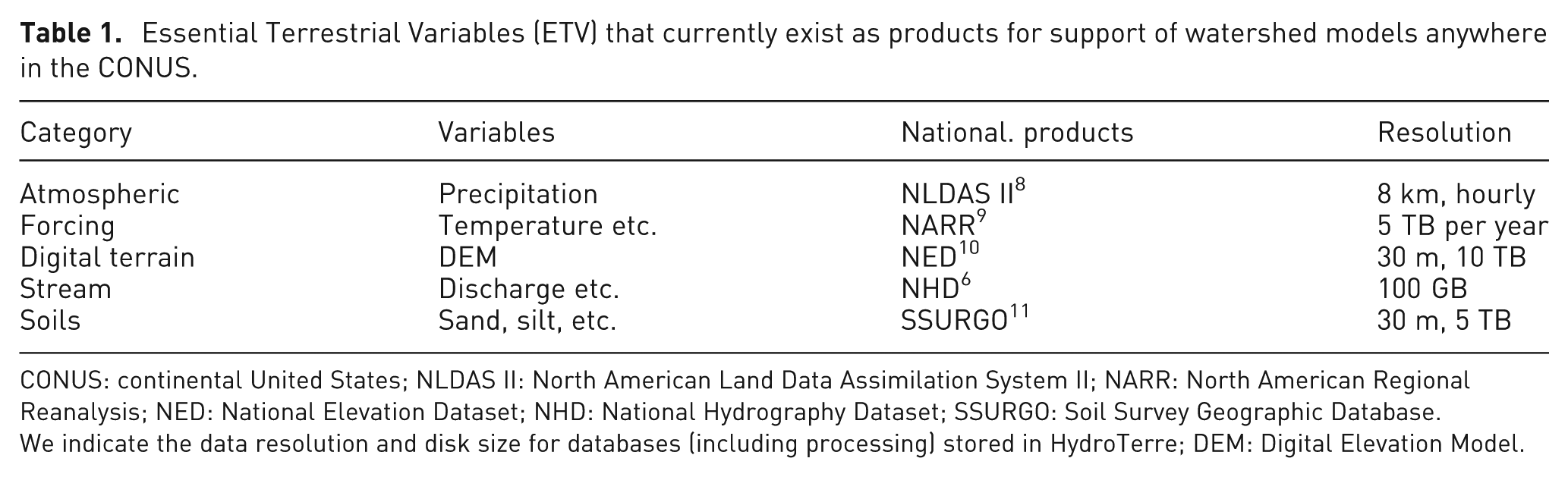
CONUS: continental United States; NLDAS II: North American Land Data Assimilation System II; NARR: North American Regional Reanalysis; NED: National Elevation Dataset; NHD: National Hydrography Dataset; SSURGO: Soil Survey Geographic Database
We indicate the data resolution and disk size for databases (including processing) stored in HydroTerre; DEM: Digital Elevation Model.
ETV data requirements for modeling watersheds at HUC-12 scales.
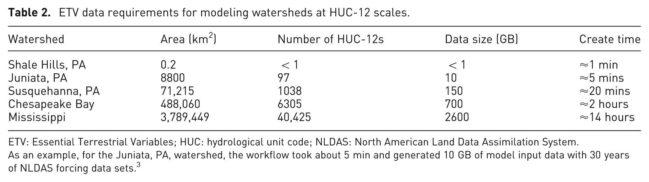
ETV: Essential Terrestrial Variables; HUC: hydrological unit code; NLDAS: North American Land Data Assimilation System.
As an example, for the Juniata, PA, watershed, the workflow took about 5 min and generated 10 GB of model input data with 30 years of NLDAS forcing data sets. 3
The second graph scale is using the National Hydrography Dataset (NHD) streams. 6 There are 29,560,501 named NHD v2.1 stream objects with hundreds of attributes required for hydrological modeling. However, when each stream object is divided into nodes (polyline vertex) and edges (polyline connections), the resultant CONUS graph has 683,298,991 unique nodes and 851,265,305 edges using the existing digitized geometry. In hydrology, edge directions are important for determining the water flow direction of a stream and these large graphs require validation. Our vision is to serve data for models, such as the Penn State Integrated Hydrologic Model (PIHM) 12 anywhere in the CONUS at any scale.
Related work
In recent years, a number of hydrological web-based visualization service-oriented applications have been developed that use site-specific study sites for sharing data. As one example, the Iowa Flood Information System provides access to flood inundation maps with real-time flood conditions and flood forecasts for gauges and sensors throughout the state of Iowa, USA, using web services and distributed services for data, map, analysis, and visualization.13,14 Another service includes HydroShare, with similar goals to share hydrological data and models.15,16
For a general overview of graph visualization techniques and research challenges, we refer to von Landesberger et al. 17 and Herman et al. 18 There exist several studies with large graph scales of social and Internet networks with relational datasets using simplification, matrices, and clustering visualization techniques.19–21 Although the NHD data products we use contain relational datasets, graph layout and simplifications were not explored here; our goal is to retain details to inform the user in situ for decision making about edge connections. Instead, our research here focuses on designing a visual interface to reveal layers of large amounts of data with navigate, view, and filtering manipulation techniques, inspired by Kandel, Heer, and Shneiderman to handle data wrangling for large graphs in hydrology.22–26 Some of the key wrangling steps taken here include the following: (1) integrating visualization in the iterative process of diagnosing graph connection problems, (2) determining how to scale large hydrology data, (3) correcting erroneous values with constraints and automation, and (4) capturing editing and data provenance using graph workflows.
Creating large graphs for hydrology using heterogeneous national datasets
Current ETV data workflows only execute using one level-12 HUC. These workflows do not include up- or downstream watersheds. However, many models require data for watershed boundary conditions, in other words, connecting graph edges. This creates a problem with our limited resources, as when a web user selects a level-12 HUC node near the outlet of the Mississippi river, the entire upstream 40,425 nodes will be selected, resulting in tens of terabytes of ETV data (Table 2). Not only does this constrain HydroTerre high-performance computing (HPC) resources, the majority of end users cannot handle this amount of data for their modeling needs. Therefore, a graph can be used to not only selecting connecting nodes (HUC-12s) but also for trimming graph branches appropriate to both HPC limitations and user requirements. Our vision is to provide a data service that scales appropriately to retrieve ETV data at any graph size. To do this requires CONUS scale graphs as inputs to our data workflows.2,27,28
NHD, maintained by USGS, provides the spatial locations of 87,259 level-12 HUCs (v2.1) 6 and approximately 14,617,263 km of stream networks within the CONUS. Maintaining these datasets is a difficult task due to the dynamic nature of streams changing positions during the year and the variation of methods used over the past decades to digitize data. Furthermore, the datasets are used by a large spectrum of users with different requirements and objectives. Clearly, due to the large scale of these graphs, automation is critical to verify correctness. First, we explain our approach to why and how we created CONUS level-12 HUC graphs, followed by issues that require visual analytics interface-enabled expert intervention.
Method to create a CONUS graph using HUCs
NHD data structures provide an implied graph by specifying a target HUC from a source HUC, or a directed connection. Unfortunately, within the NHD graph, there are instances when targets do not exist, and thousands of connections are not touching neighbors. 28 Additionally, the NHD data structures imply only one connection when level-12 HUCs have multiple connections with adjacent HUCs. Hence, we needed to create a derived CONUS graph using NHD to resolve these problems.
The method to create a graph using CONUS level-12 HUCs with NHD geodatabases started by developing a dictionary containing unique level-12 HUC keys. 28 By treating each HUC geometry as a node, 83,016 keys were identified. Checking the target keys identified by NHD, it was discovered that 38 unique keys did not exist and were used by a total of 221 HUC-12s. 28 With a relatively low number of level-12 HUCs, it appeared that manual intervention was feasible. However, by creating a list of neighboring HUCs for each HUC, it was discovered that 1940 HUCs had target keys that did not touch the source. 28 Using our strategy not only includes multiple neighboring targets (edges), but HUCs called closed basins were also selected. Closed basins are watersheds that do not have surface streams that connect to another watershed but are needed for groundwater and lake modeling.
To determine edges and directions between level-12 HUC nodes, the intersection of each stream with HUC boundaries was calculated. Each point was then buffered (a polygon enclosing the intersection point) at 15-, 45-, 60-, 75-, and 90-m intervals, creating more points along the stream geometry. Using the National Elevation Dataset (NED) which has a 30-m resolution, elevation values were assigned to these points with the goal to determine high- and low-elevation values. This technique was not effective due to inadequate elevation resolution, short stream reaches, lack of smooth stream reaches, and/or watershed boundaries, and the large number of flat-sloped areas at these intersections.
Instead, the chosen solution was to live with dirty data by assuming that the digitized direction is from down- to upstream and then identify edges that require direction corrections. These corrections were identified by creating upstream depth-first search (DFS) graphs at all major river outlets (root nodes) and identifying holes within the generated polygons. The DFS-generated polygons were then automatically compared with well-known large-watershed boundary polygons for verification. See Leonard and Duffy 28 for further details and here we demonstrate our DFS graph process with the Juniata watershed shown in Figure 1.
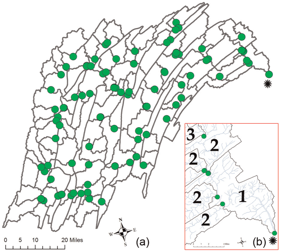
(a) By selecting the root HUC-12 node (asterisk), using DFS or BFS algorithms, 97 HUC-12s are selected that form the Juniata watershed. The green circles mark the locations where edges connect to adjacent HUC-12s (watershed outlets) and (b) the insert shows the streams (light blue) and the numbers denote graph distance from root node.
Why corrections require expert intervention
The above approach to create upstream graphs is successful for major river basins without restriction on graph size, as we can identify holes within watershed polygons. However, our goal is to use the graph to create dynamic graph sizes anywhere in the CONUS where we cannot rely on holes to determine missing HUCs. For example, we have access to a 64-node HPC cluster and we want to restrict the graph to 64 level-12 HUCs at a time, with 64 being considered changing as we follow the path of a major storm. From experiments conducted with the Juniata watershed (Figure 1), it became apparent that our assumption that the digitized direction (down- to upstream) was not sufficient and required too many expert edits.
The most common reasons for expert intervention at the level-12 HUC scale included conflicting edge directions, edges that pass back and forth along HUC boundaries, and edges within flat-sloped elevations as summarized in Figure 2(a). The number of corrections was in the thousands at the CONUS scale by treating each HUC as a node and focusing at the connection locations only. The next logical progression is to search beyond the intersection locations and buffered intersections, by following the entire length of the stream in both directions to determine the correct flow direction.
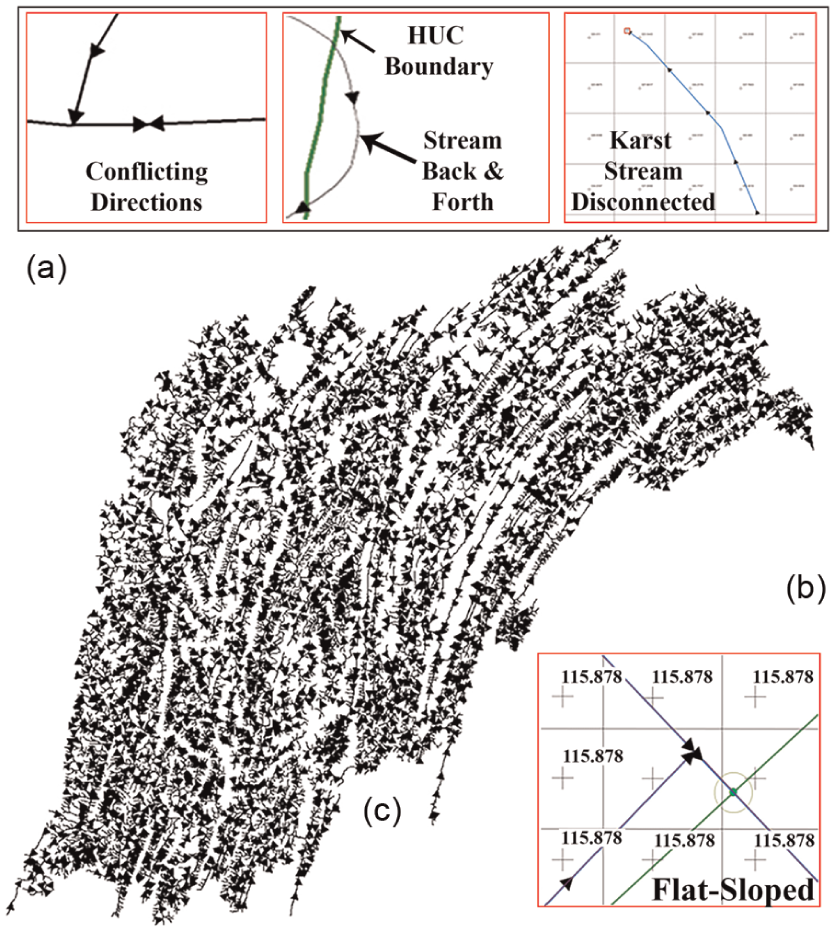
(a) Examples of edge direction issues, (b) streams within same elevation values, and (c) Juniata edge directions.
To search from the intersection requires a corrected stream network at the CONUS scale. There are 29,560,501 named NHD v2.1 6 stream objects in the CONUS, but when every edge is split into individual segments with existing digitized vertices, there are 851,265,305 edges and 683,298,991 nodes. Table 3 summarizes graph sizes with various scale watersheds within the CONUS. This shows that there are hundreds of thousands of the same issues as are summarized for one example in Figure 2(a). Additional issues found include streams that are disconnected (that happen in karst environments characterized by underground drainage with sinkholes and caves) and streams interconnected with human-made canals that change natural flow directions. Many of these issues require expert intervention as there is a lack of elevation detail that would be required to make corrections automatically.
Graph sizes for various watershed scales.
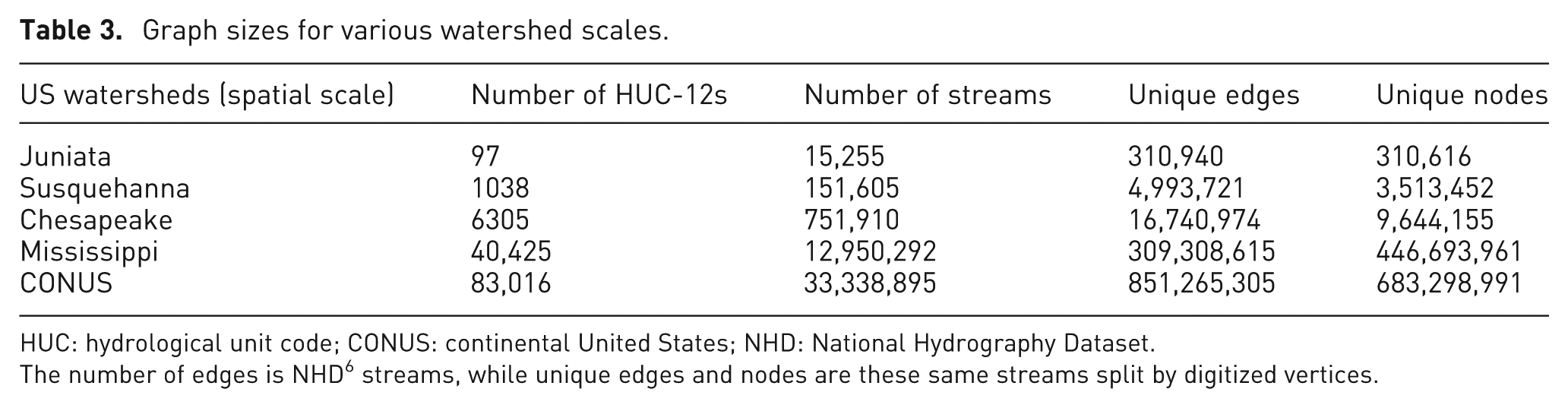
HUC: hydrological unit code; CONUS: continental United States; NHD: National Hydrography Dataset.
The number of edges is NHD 6 streams, while unique edges and nodes are these same streams split by digitized vertices.
The NED resolution is 30 m, which is not sufficient to automatically correct and verify flow directions. The gridded lines in Figure 2 indicate the elevation value for the entire rectangle. Clearly, when so many stream vertices share the same elevation value, determining direction is problematic, especially when there are multiple streams in the same region with conflicting directions (Figure 2(b)). The reader may suggest to determine directions for connecting edges by searching further than the intersection location and use the result to judge the likelihood direction. Unfortunately, as described earlier, there are hundreds of thousands of issues with the stream networks. Instead, we propose a two-tier solution by having expert intervention at the HUC intersections first, followed by validating stream networks within each HUC to create a valid graph.
Visual analytic objectives
Since resolution of available elevation data does not support full automation to address issues with stream networks, we propose a visual analytics approach that leverages expert knowledge. We illustrate the approach for the Juniata watershed. Figure 2(c) illustrates the 15,255 streams or 310,940 edge segments within the Juniata watershed (Table 3). The arrowheads indicate the direction of each edge. Clearly, by visual inspection, determining which edge directions are correct or not is a time-consuming and tedious task, even with a relatively small watershed size. Following the visual analytics mantra, 29 we propose that our visual analytics tools do the following to create and validate large graphs for hydrological modeling using national datasets:
Analyze first. Using graph workflows, the watershed graph will be analyzed to identify (1) level-12 HUCs that have streams with no elevation changes (flat-sloped), (2) conflicting edge directions, and (3) possible outlet nodes.
Show the importance. Directions at flat-sloped streams for HUC watershed outlets are the most important features to validate first, as these errors propagate up and down the entire CONUS graph.
Zoom, filter, and analyze further. Due to the large number of stream segments (Table 3), it is unrealistic to expect a user to find edges by interacting with geographic information system (GIS) maps. Tools need to provide suitable zooming and filtering settings for efficient analysis.
Details on demand. Visualizations such as Figure 2(c) with too much detail are tedious to interact with for users. It is important to reveal data at appropriate spatial scales and provide control to users to have data and details on demand.
As we demonstrate in the next section, visual analytics is critical to direct users efficiently to specific locations for validation and iterate over large graphs using heterogeneous CONUS national datasets.
Visual analytics workflow to resolve large graphs for hydrology
The previous sections described two graph scales for hydrological modeling within the CONUS. The first scale treated each level-12 HUC as a node, which generates a graph size of 83,016 nodes and 157,802 edges. The second scale is the CONUS stream network with a graph size of 683,298,991 nodes and 851,265,305 edges. To solve the large graph scale, it is first necessary to resolve the edge directions at the level-12 HUC scale, followed by the internal edges within each HUC. In this section, we describe the workflows to implement these steps using the Juniata watershed as a use case. First, we show how large graph workflows are created and are used for automated analysis within the HydroTerre cyberinfrastructure. Second, we show the design of the visual interface to engage the expert user to resolve graphs for their own modeling goals using pre-defined actions for common graph issues.
HydroTerre workflow overview
HydroTerre workflows are initiated via the web application by selecting a level-12 HUC. HydroTerre consists of four workflows forming an end-to-end workflow system for hydrological modeling (Figure 3(a)) in a distributed computing environment.3,4 First is the ETV data workflow, responsible for selecting, projecting, clipping, and extracting data within the level-12 HUC watershed. 1 A typical level-12 HUC data bundle contains standard GIS datasets and typically takes about 2 min to create.1,27
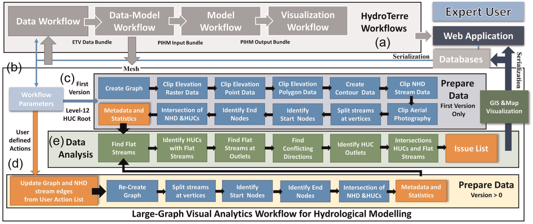
(a) The HydroTerre end-to-end workflows, (b) the graph workflow, (c) automated large graph data generation process using national data products, (d) large graph corrections with user-defined actions, and (e) automated analysis of the graphs to identify issues that require expert intervention and populates user interface controls.
The ETV data workflow operates as an independent service using file formats common for many models. Conversely, the data-model workflow is dependent and employs the ETV workflow service as data inputs. Four parameters control the watershed level-12 HUC boundary and stream topology that in turn controls unstructured mesh details for hydrological modeling. 2 The data-model workflow assigns land-use, initial conditions, and other parameters using the national datasets as a priori values.
The PIHM-model workflow consumes the data-model workflow as data inputs. Using the web application, calibration, initialization, and HPC model parameters are controlled by the expert user. Default values are automatically assigned using data-mining strategies from the previous workflow results. The ETV, data-model, and model workflows have been executed millions of times to investigate the main reasons for failure within the national datasets, or within the models.2,3
The last HydroTerre workflow is the visualization workflow to encourage iterative and investigative processes by the expert user to rapidly change data-model and model parameters. 4 The visualization workflow consumes the data, data-model, and model workflow services as data inputs. This workflow provides maps and data visualizations that allow the expert user to drill-down, interrogate model results, and rapidly test and re-submit hydrological models for further analysis.
Graph workflow overview
The end-to-end workflow described earlier considers an individual level-12 HUC at each phase. The purpose of the graph workflow is to provide the ability to create a dynamic number of level-12 HUCs from a root node. For example, an expert user is interested in following a storm path or the path of a major river basin near a particular town (root node). The other purpose is to provide analysis of the graph networks within these level-12 HUCs and identify issues, with inconsistent edge directions the most common issue.
In practice, we would expect flow direction to be consistent in one direction, from higher (mountains) to lower elevations (oceans). For models such as PIHM, when edge directions meet, the model solvers will either not converge or be inefficient causing simulations to be slower. Based on the analysis of executing workflows, 1.5 million times with CONUS level-12 HUCs, data-model workflows (responsible for transforming ETV data to PIHM inputs) failed 26.91% of the times due to poor graphs.2,3 The stream graph is essential for generating PIHM meshes and incorrect graphs account for 70.66% of model workflow failures.2,3
HydroTerre, PIHM, and other hydrological models require verified graphs at both level-12 HUC node and edge scales. However, every model and expert user has different requirements and strategies to analyze these graphs. Therefore, the graph workflow has been designed to be loosely coupled to accommodate these strategies, rather than directly incorporate them into the data workflow (Figure 3(a)). First, we explain the automated steps to create and analyze large graphs for hydrological modeling.
Graph workflow automated steps
Figure 3(b) summarizes the main components of the graph workflow and how it is incorporated into the HydroTerre end-to-end workflow system. From the web application, once the user initiates the workflow, a new job record is created in the database storing the graph workflow properties as summarized in Table 4. This object is used for provenance and reproducibility by storing all workflow parameters selected by the user and those that are automatically generated by the graph workflow for the user interface. The workflows are executed in a distributed compute environment; therefore, this job record is used to serialize and de-serialize properties for both the graph workflow and the web application interface.
The graph workflow job object stored when user execute workflows.
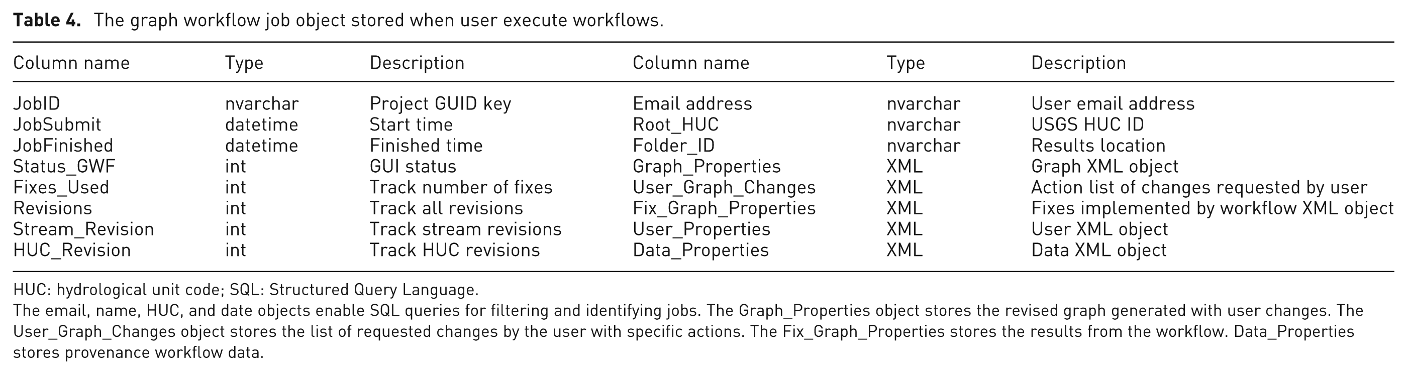
HUC: hydrological unit code; SQL: Structured Query Language.
The email, name, HUC, and date objects enable SQL queries for filtering and identifying jobs. The Graph_Properties object stores the revised graph generated with user changes. The User_Graph_Changes object stores the list of requested changes by the user with specific actions. The Fix_Graph_Properties stores the results from the workflow. Data_Properties stores provenance workflow data.
Within the graph workflow, there are two main steps: data preparation and data analysis. Data preparation is partitioned into two sections based on the revision of the graph workflow. When a user defines the graph properties (described in section “Interface for graph visual analytics workflow”) for the first time, the components in Figure 3(c) are executed. Briefly, these create a level-12 HUC graph, followed by clipping elevation, stream, and aerial datasets. The NHD stream networks are then divided into edges and nodes, followed by finding the geolocation of the intersections between HUCs and the graph edges. Statistics and metadata about each of the data products generated are created for populating user interface controls and data detail on demand. These metadata are stored in the graph job record in the HydroTerre databases.
The second partition (Figure 3(d)) of data preparation implements the user-defined actions (described in section “User actions to correct graphs”) to correct graphs and stream networks based on a previous graph version. Using the web application, the user creates a list of actions he or she wants to perform (described in section “Interface for graph visual analytics workflow”) either with the level-12 HUC connections or with the stream networks. To improve performance, most of the data preparation done in the first partition is not re-executed when not affected by any corrections to graph edges.
The second step is data analysis (Figure 3(e)), which happens after each data preparation component. This step identifies actions required by the user to address their modeling requirements. The main components are finding flat-sloped edges within level-12 HUCs, flat edges at HUC outlets, and edges with conflicting directions and root nodes (outlets). The last component of this step is to collate these automated data analyses into the User_Graph_Changes object (Table 4) to populate user controls within the web application.
After the second step, a new versioned map visualization is generated for the user to analyze the impact of their requested changes. Briefly, the GIS and map visualization step prepares data symbology and creates a map service using ESRI ArcGIS Server software development kits. 30 What this map step does is explained in further detail within the interface design section “Interface for graph visual analytics workflow.” First, we explain what the user actions are to correct graphs, as the design and symbology used in maps are dependent on the results of user actions.
User actions to correct graphs
The previous section describes the automated analysis of level-12 HUCs and stream networks based on user parameters to create a large graph. One of the data products generated is an issue list that populates the interface to inform the user of possible changes required for the large graph. The user is required to specify an action for each issue identified by the automated analysis. These methods have been broken into five common actions:
Delete. Some stream edges that increase mesh complexity (such as very small triangles and slivers3,31) also increase solver compute times without improving hydrological understanding. Therefore, it is necessary to delete nodes and/or edges. Additionally, some networks (karst, Figure 2(a) sinkholes) are not attached and require deletion for some model applications.
Reverse. Edges with directions upstream need to be reversed without changing vertex locations. When edges cross level-12 HUC boundaries, then the entire HUC graph is recomputed. Edges within the HUC, only the sub-graph, are recomputed.
Ignore. Depending on the model requirements, there are circumstances when graph nodes and edges can be ignored. For example, models that can handle karst (caves) streams.
Assign heights. For flat-sloped edges, it is necessary to modify node elevation values. The expert user can assign elevation values manually or assign slope from start or end vertices of the flat-sloped edges.
Confirmed. The direction of flat-sloped edges at level-12 HUC outlets requires confirmation by the user.
As discussed previously, the user will need to verify the large graphs at two scales: the first scale is at the level-12 HUC, followed by the stream networks within each HUC. At the level-12 HUC scale, the expert user is required to validate HUCs with flat-sloped outlets. The direction of these edges requires confirmation; otherwise, the user will need to decide direction from the above actions. To validate stream networks within each HUC, we have identified the following problem types during the automated graph workflow (Figure 3(e)) that require intervention by the user via the visual interface.
Inconsistent edge direction. As shown in Figure 2(a), we can automatically identify nodes with edges that meet using a simple graph traversal algorithm of searching for edges that have the same terminating node. These are automatically corrected when there is sufficient elevation data; otherwise, the user can identify which edge is incorrect and reverse the edge.
Sub-graphs. Sub-graphs are common for streams in karst (sinkholes, caves) landscape environments (Figure 2(a)). However, some models expect simple graphs. When data support, the user can ignore these edges if their model can handle multiple graphs, otherwise delete them.
Incorrect outlets. There are edges that are topologically correct and appear valid from visual inspection. However, there are circumstances where the stream does not follow the lowest elevation values, for example, deep river gullies. 3 Therefore, the flow direction has water going upstream creating sub-graphs. These appear as root nodes. The user can ignore, delete, reverse the edges, or assign new heights after analyzing detail on demand.
Flat streams. All edges that are flat-sloped within the level-12 HUC are identified for the user to correct, if their models require edges with slope. Users can ignore these edges or assign heights using the above actions.
The above actions are automatically serialized and stored in databases for provenance and reproducibility within the User_Graph_Changes XML object (Table 4). How users generate these actions to address issues with graph workflows and user interfaces are discussed next.
Interface for graph visual analytics workflow
There are two main steps for the user to analyze large graphs using the visual analytics workflow. The first step (Figure 4(a)) is to create a graph from a root level-12 HUC. The user can select a root HUC via the map using the pick tool (Figure 4(b)), by unique identification or by name (Figure 4(c)). The user specifies the level-12 HUC data source (Figure 4(d)) followed by specifying how to select graphs up- and downstream from the root HUC (Figure 4(e)). There are currently three selection methods: DFS, which selects level-12 HUCs along the dominant stream path first, or the user can specify breadth-first search (BFS) to select HUCs closest to the root HUC first, and the remaining option is to select none.
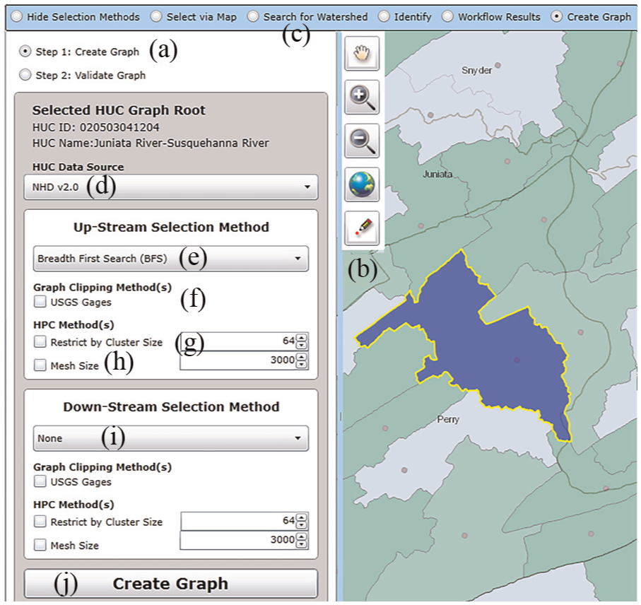
To create a large graph for modeling, the main steps are to specify the up- and downstream graph properties from the root node (blue polygon) and methods to clip the graph.
As already discussed, using DFS or BFS searches can create very large graphs that our current cyberinfrastructure cannot support. Therefore, we provide two methods to clip graphs. The first method is to clip graphs at USGS gauges (Figure 3(f)). USGS gauges provide datasets (temperature, etc.) that can be used for hydrological model boundary conditions. For example, if a modeler is interested in following the path of a major flood, he or she can direct HPC resources downstream from the root node (USGS gauge) rather than modeling the watersheds upstream.
The second method is to clip graphs using HPC requirements. There are two options. The first is to restrict the graph by the number of HPC cluster nodes up and downstream (Figure 4(g)). For example, a user has access to a 128-node cluster; he or she can split the up and downstream graph to 64 nodes each. The second option is to restrict the graph by mesh size (Figure 4(h)). During the data-model workflow (Figure 3(a)), meshes are created representing the land surface. When meshes are large, models like PIHM require more HPC resources that may take too long to compute. Hence, we provide this clipping method to aid the modeler to select graph HUCs up to the mesh size of choice, up- and downstream from the root node. All clipping methods can be used in conjunction with each other to create graph selections for different modeling strategies. For our Juniata watershed use case, we used the map point tool to select root node “020503041204.” To replicate the graph of Figure 1, no downstream selection method was chosen (Figure 4(i)) and BFS search was used to select upstream HUCs with no graph clipping (Figure 4(e)).
After specifying up and downstream clippings and selection methods, the user initiates the first version of the graph workflow by clicking on the create graph button (Figure 4(j)). The graph selection methods specified by the user are serialized and assigned to a new graph workflow object (Table 4) in the HydroTerre databases. The compute node executing the graph workflow de-serializes these properties and executes the workflow as described in section “Graph workflow automated steps.” The graph workflow generates an issue list and metadata to populate the user interface and map visualizations. Figure 5 shows the map workflow result and Table 5 summarizes the issue list, data products, and compute times for the Juniata watershed.
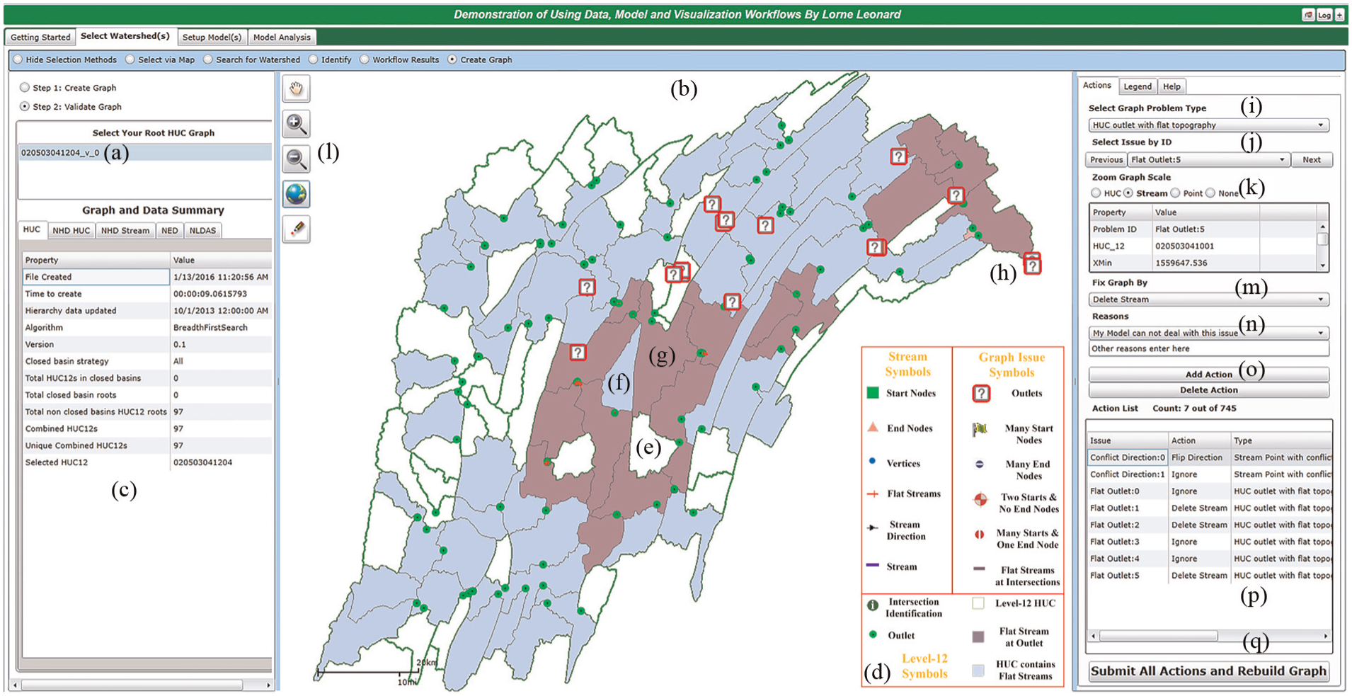
The visual analytics interface to validate the Juniata watershed. The left panel allows users to select graph workflow versions and interrogate the graph and data metadata. The middle panel map shows the graph results, nodes, and edges, with colors and symbols to assist the user to identify problems. The right panel identifies graph issues and controls automated zoom to level of detail. The user creates an action list to fix the graph for modeling.
The main steps for data preparation and analysis of the Juniata graph workflow are summarized below.
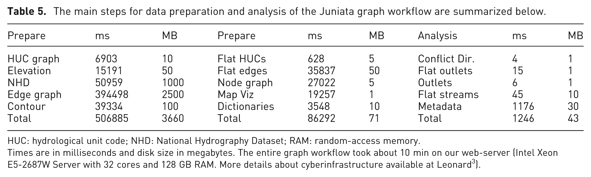
HUC: hydrological unit code; NHD: National Hydrography Dataset; RAM: random-access memory.
Times are in milliseconds and disk size in megabytes. The entire graph workflow took about 10 min on our web-server (Intel Xeon E5-2687W Server with 32 cores and 128 GB RAM. More details about cyberinfrastructure available at Leonard 3 ).
The expert user selects the versioned graph from a list shown in Figure 5(a), which reveals the graph as a map (Figure 5(b)) and populates two user controls. The first control summarizes the graph and metadata properties of the Juniata graph generated by the user (Figure 5(c)). This control provides information about the graph method used, properties about HUCs, streams and supporting datasets, such as NED. These metrics are useful to determine the data requirements, such as forcing datasets, 27 required to execute the end-to-end HydroTerre workflows. To prevent the user being overwhelmed with data, details are not revealed at the first map scale. Rather, the important issues are highlighted with colors and symbols at multiple zoom scales as summarized in Figure 5(d). For example, level-12 HUCs with green edges and white fill indicate no problems (Figure 5(e)), HUCs with blue fill indicate flat-sloped streams and are located within the HUC (Figure 5(f)), and purple HUCs have flat-sloped streams at the outlet (Figure 5(g)). These purple HUCs, numbered in suggested order of correction by distance from a root graph, are suggested to be addressed first by the user to validate the edge direction, as upstream connections may be incorrect affecting the entire graph structure. To aid the user in identifying the locations of the outlets at each HUC, small green circles designate their location without showing edge geometry at this scale extent. Furthermore, there are question mark symbols at each of the outlets that require validation by the user. Based on our graph selection, we know there should be only one outlet, not 16 as the automated analysis revealed.
The second control serves three functions. The first is a help guide, explaining the types of issues and strategies to validate graphs. The second is a map legend that aids users to control level of detail by turning data layers on or off and controlling transparency. The third function is a means to create an action list to validate the graph. The user specifies a problem type he or she wishes to address (Figure 5(i)), which will then fill in the issue by identification control (Figure 5(j)). This control automatically zooms the map to the issue at hand, rather than the user zooming into the map by themselves. The user can override this zoom action at three (HUC, stream (edge), and point) scales (Figure 5(k)). Additionally, the user can control the map with typical zoom and pan tools (Figure 5(l)). Each zoom scale reveals different amounts of data for the user, with point scale revealing all data and then as the zoom extent increases, less data are shown to the user. For example, for a user trying to resolve flat-sloped streams, at the edge scale, elevation values per vertex are labeled, but not NED grids. At the HUC scale, flat-sloped streams are purple lines to alert the user to a data problem requiring attention.
The next step is to select an action (Figure 5(m)) as described in section “User actions to correct graphs” to fix the graph. For provenance, the user has to specify a reason for their action (Figure 5(n)) before adding the action (Figure 5(o)) to the list of actions (Figure 5(p)). The last step is to submit all actions and rebuild the graph (Figure 5(q)). The action list is serialized and added to a new versioned graph workflow job as described previously. A new graph workflow is generated and the user repeats step 2, graph validation, until all issues (old and potentially new issues) have been resolved. For models like PIHM, the 745 issues first identified for the Juniata watershed require modification by the user to improve model performance and took about 2 h to create a corrected large graph. Clearly, even for a small number of level-12 HUCs, fixing these issues is time-consuming and tedious when using standard GIS techniques of manually interacting with map and data taking days to complete corrections. Our graph workflow that automates finding graph issues, combined with visual analytics tools that enable users to zoom directly to the problem and quickly assign an action fix from pre-defined solutions, makes the task of resolving CONUS scale graphs feasible.
Conclusion and future work
Providing the ability to work with large graphs is essential to improve hydrological science. We demonstrated the challenges of working with two scales of imperfect graphs using heterogeneous CONUS datasets; as outlined, imperfect graphs are the norm, not an exception. The first scale discussed was using NHD level-12 HUCs as nodes and the second scale with dividing the NHD CONUS stream network into segments (683,298,991 nodes and 851,265,305 edges). We discussed our techniques to create derived graphs using NHD and demonstrated why expert intervention is necessary to validate these graphs with the dominant reason being lack of elevation detail to validate edge directions. To assist the expert, we then discussed our graph workflow to prepare and analyze data for hydrological modeling. These results were then used to populate the visual analytics interface. We then showed how with user actions (delete, reverse, and assign heights), the expert user addresses graph problems such as inconsistent flow direction, outlets, and flat-sloped streams.
In our Juniata case study, although we demonstrated how our interface simplifies the process to correct issues, the large numbers of issues to correct (745 issues) are still challenging for expert users to cope with. We hope that using LiDAR elevation products may reduce the number of issues in particular with correcting elevation values along streams. However, LiDAR will significantly increase the CONUS scale graph by many orders of magnitude and visual analytic methods will be critical to resolve these large graphs for hydrological modeling. Our vision is to minimize the number of corrections by (1) improving the workflow computational performance for faster interface responses by the user; (2) as more users interact with our graph workflows, the stored provenance and reproducibility of our workflows will improve subsequent user experiences by automatically sharing existing corrections stored in our databases. However, sharing existing corrections raises the question about accuracy with user-generated graphs. Therefore, further research will also include conducting experiments with multiple hydrological models to measure success rates with user actions and specific goals with our interface design. We hope lessons learned from these experiments will improve accuracy as well as improve our automated strategies.
This article focuses on repairing flow directions with NHD stream graphs under normal flow conditions. We anticipate additional uses for the corrected graphs, such as assigning soil properties to missing sand, silt, and clay percentages found adjacent to streams. 3 These are necessary for models such as PIHM, as well as retrieval of elevation cross sections along the stream graphs for flood plan analysis.
Footnotes
Acknowledgements
The authors would like to acknowledge the support from Professor Christopher J Duffy at the Department of Civil Engineering.
Funding
The author(s) received no financial support for the research, authorship, and/or publication of this article.