A fast feature vector approach for revealing simplex and equi-correlation data patterns in reorderable matrices

Abstract

Reorderable matrices may be used as support for tabular displays such as heatmaps. Matrix reordering algorithms provide an initial permutation of these matrices, which should help to reveal hidden patterns in the dataset in the visual structure. Some of these algorithms directly permute the data matrix, instead of its row- and column-proximity matrices. We present a data matrix reordering method (feature vector-based sort – FVS), which reorders a data matrix aiming to reveal simplex and equi-correlation patterns. Our approach extracts feature vectors from a data matrix and uses them to calculate row and column permutations of the data matrix. We used FVS for reordering data matrices of distinct real-world scenarios, in which it revealed those patterns. Our experiments with synthetic matrices revealed that FVS is faster than other known matrix-reordering algorithms and produces results of approximately the same quality (in terms of stress function) when these patterns are hidden in the data matrix. We also present some real-world datasets reordered by our algorithm and discuss the patterns that it uncovers.

Keywords

Reorderable matrix data canonical patterns seriation

Introduction

One aim of information visualization techniques is to reveal patterns in datasets. A dataset may be represented as a matrix or table, whose cell values are related to a tuple (matrix row) and a field (matrix column). A background color may be defined for each cell according to its value. This definition transforms the matrix into a heatmap, whose colors may help users to identify patterns in data. Bertin¹ proposed the concept of a reorderable matrix as a matrix that supports row and column permutations. If reordering is done appropriately, a heatmap based on a reorderable matrix can reveal hidden patterns. Given the factorial number of all possible permutations of rows and columns, much research has been done in order to provide good reordering algorithms for data originating from areas such as archaeology, cartography, and bioinformatics.²

In this sense, Wilkinson³ defined five canonical data patterns for matrices, which expose clear relationships between row and column elements of a matrix: simplex, equi-correlation (or equi), band, circumplex, and block. Figure 1(a) and (b) exemplify equi and simplex patterns, which we cite throughout this paper. In this figure and most figures in this paper, darker heatmap cells represent values closer to 0, and lighter cells represent values closer to 1 (in a normalized version of these patterns). In order to illustrate these examples, suppose that both matrices in Figure 1 represent grades (colors) of students (y-axis) in subjects (x-axis). In this context, an equi pattern (Figure 1(a)) indicates that each student has approximately the same grades in each subject, in a gradient from bad to good grades (top to bottom rows). A simplex pattern (Figure 1(b)) indicates the same gradient (reversed from bottom to top), but also a gradient from easiest to hardest subjects (rightmost to leftmost column).

Figure 1.

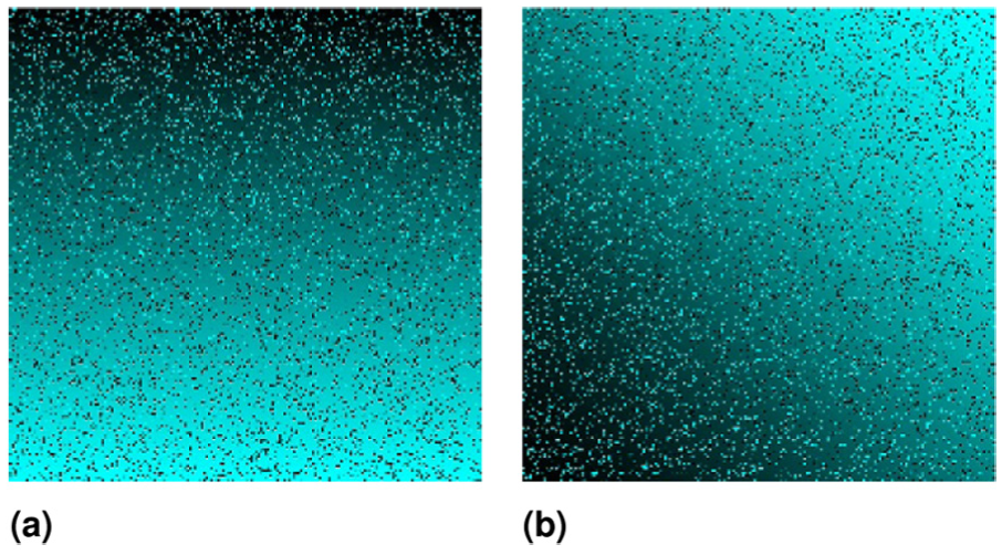
Heatmaps with some data canonical patterns. (a) Equi pattern (noise level: 20%). (b) Simplex pattern (noise level: 20%).

There are lots of algorithms that reorder a data matrix based on creating and permuting their related proximity matrices (i.e. similarity or dissimilarity matrices) for rows and columns. However, the possibility of creating algorithms to reorder a data matrix without creating proximity matrices seems to be under-explored; also, we only found a few comparisons regarding these kinds of algorithms.

This paper presents a new matrix reordering algorithm that does not require proximity matrix construction. It aims to reveal simplex and equi patterns if they are present in some data matrix permutation. The new method is faster than other analyzed methods. In order to discuss our method, we first present a brief theoretical background about matrix patterns and quality measures, and then we present related research on matrix reordering algorithms. “Method” formalizes our method, and “Results and discussion” discusses the results of matrix reordering experiments on synthetic and real data.

Theoretical background

This section details simplex and equi patterns,³ and also presents information about measurements of the quality of a permuted matrix.

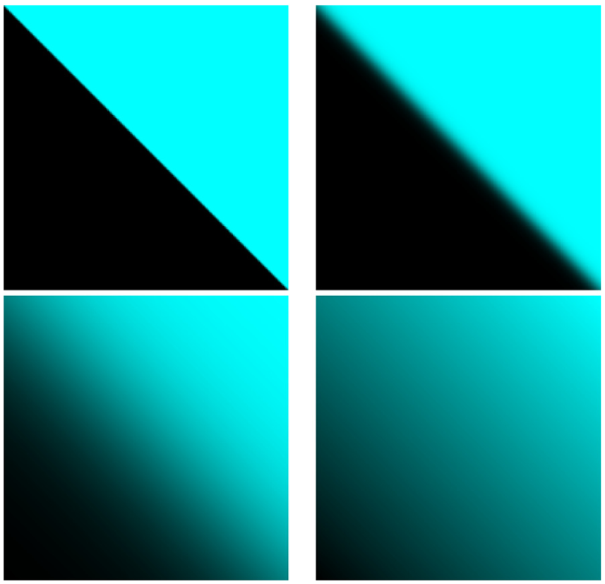
Given a matrix $X_{n \times p}$ that obeys a simplex pattern, each of its cells is defined as $x_{ij} = e^{t} / (1 + e^{t}) + u_{ij}$ , where $i = 1, \dots, n$ , $j = 1, \dots, p$ , and $t = (j / p - i / n) / b$ . In this expression, b defines the smoothness of the boundary between the regions of the highest and lowest values of the data matrix. Figure 2 exemplifies four distinct values of b for this pattern.

Figure 2.

Simplex pattern without noise and with distinct smoothness values: (a) $b = 0.002$ ; (b) $b = 0.02$ ; (c) $b = 0.2$ ; (d) $b = 2$ .

Parameter $u_{ij}$ is a random error. Wilkinson³ defines it as $u_{ij} = k e^{(- t^{2}) Z}$ , where Z is a standard normal random variable. Our approach replaced this definition with salt-and-pepper noise.⁴

On the other hand, each cell $x_{ij}$ of a matrix X that obeys the equi pattern has value $x_{ij} = bi / n + u_{ij}$ . Here, parameter b does not affect smoothness, but the scale of $i / n$ . Note that if we take two equi matrices with distinct values of b, their normalized versions will return similar values (in spite of noise). This fact impacted design choices for our evaluation procedure, as we explain later.

Matrix evaluation may use distinct approaches.⁵ Here we used stress of the Moore neighborhood⁶ (or Moore stress, for short) and the minimal span loss function (MSLF).⁵

Moore stress considers horizontal, vertical and diagonal neighbors of each cell. Moore stress for a matrix $X = {x_{i, j}}$ is given by $s = \sum_{i = 1}^{n} \sum_{j = 1}^{m} \sum_{k = - 1}^{1} \sum_{l = - 1}^{1} (x_{i, j} - x_{i + k, j + l}) .$ The lower the value of s, the better the provided reordering.

MSLF is a function given by $m = \sum_{k = 1}^{n - 1} d_{k, k + 1}$ , where $D = {d_{i, j}}$ is a distance matrix of rows (or columns) i and j. D is constructed by using a distance measure. In this paper, we opted for using Euclidean distance as the classic distance measure. MSLF is equivalent to the sum of distances of all neighboring rows (or columns). The lower the value of m, the better the permutation.

Given a matrix that evidences the equi or simplex pattern (without noise), and one of its permutations in which this pattern is not evident, values of both evaluation measures are lower in the former (given the high similarity among neighboring rows and columns) than in the latter.

Related research

Some matrix reordering algorithms reorder proximity matrices. Therefore, they must permute row and column similarity matrices, and then they must apply these permutations to the original data matrix. Similar approaches consider proximity matrices of rows or columns as a graph adjacency matrix, and therefore they try to order nodes of this graph. We call both types proximity matrix reordering algorithms. On the other hand, some algorithms permute rows and columns of a data matrix without creating proximity matrices. We call them data matrix reordering algorithms.

Proximity matrix reordering algorithms

Proximity matrix reordering algorithms are based on distinct approaches. Breadth-first search, depth-first search, reverse Cuthill–McKee, King’s algorithm, Degree,⁷ visual assessment of (cluster) tendency,⁸ OREO,⁹ TSPCluster¹⁰ and EM-ordering¹¹ are graph-based algorithms, which order graph nodes according to specific searching procedures (e.g. breadth-first search) or node characteristics (such as node degree or node similarity).

Some of them model matrix reordering problems as a traveling salesman problem (TSP), where cities are rows (or columns) and their distances are weighted edges. OREO⁹ is a biclustering approach which defines that either a TSP model or a network flow model may be used to reorder matrices appropriately. EM-ordering uses a specific TSP solver to discover matrix permutations that minimize entropy.¹¹ TSPCluster¹⁰ also uses a TSP solver to solve the reordering problem for a given number of clusters.

There are also other clustering-based approaches which are applicable to proximity-based matrix reordering. Elliptical seriation¹² works with clustering supported by convergence properties for sequences of iteratively formed correlation matrices. Chen and Saad¹³ proposed approaches for reordering adjacency sparse matrices of a graph (by clustering their similarity matrices), in order to extract dense subgraphs. Bar-Joseph et al.¹⁴ order the leaves of a hierarchical clustering tree in an optimal linear ordering, where leaves are rows (or columns) of a data matrix.

It is worth noting that detecting cluster boundaries is useful for clustering purposes, but it is not always of concern for matrix reordering. Besides, Wilkinson³ argues that there is “no advantage to using cluster analysis for seriation or matrix permutation unless the point of the display is to document a cluster analysis already used for other reasons”.

Multidimensional scaling (MDS), singular value decomposition (SVD), locality preserving projection (LPP)³ and multi-scale¹⁵ are based on linear algebra and dimension reduction. Given a set of n rows (or columns) of a data matrix, their general approach has two main steps: creating a $n \times n$ proximity matrix, whose rows are considered as sets of n-dimensional points; and reducing the dimension set to a single dimension, which provides an ordering of the n rows (or columns).

Branch-and-bound algorithms may be applied to proximity matrices in order to reduce bandwidth, but scalability issues seem to arise for more than 40 rows (or columns).¹⁶ Ant-colony-based optimization is another proximity matrix reordering approach.¹⁷

Data matrix reordering algorithms

Data matrix reordering algorithms include heuristics, clustering and entropy-based approaches. 2D Sort¹⁸ aims to “build black areas to the top left and the bottom right corners of the matrix”; it iteratively sorts rows (or columns) according to the sum of their values weighted by column (or row) position.

Barycenter heuristic¹⁸ (BH) binarizes a matrix with a user-defined threshold and uses this binarized matrix as a bipartite graph adjacency matrix. Then the algorithm applies a crossing minimization step which permutes both graph partitions, and uses these permutations in the data matrix.

Ben-Dor et al.’s biclustering algorithm¹⁹ uses a probabilistic model that helps find order-preserving submatrices (OPSMs) inside a data matrix. An OPSM is a local pattern whose columns have at least one permutation that forces the values of each row to be in an ascendant order.

PQR Sort²⁰ is a binary matrix reordering algorithm based on PQR trees. A PQR tree imposes a set of constraints (or restrictions) on a permutation space in order to define consecutiveness among the elements of this set when possible. This concept is used to force rows (or columns) to stay together when they are similar. The tree frontier (i.e. its leaves, from left to right) reveals a possible order for rows (or columns).

Bond energy algorithm (BEA)^21,22 tries to maximize a measure of effectiveness; it is capable of revealing band and block diagonal patterns, and also other partitions not conforming to block diagonal.

None of the data matrix reordering approaches surveyed used feature vector analysis. Also, some of them focus on revealing a specific pattern of the data matrix. We highlight two works that compare matrix reordering algorithms aiming to reveal simplex and equi patterns. Wilkinson³ compared MDS, SVD, LPP and clustering. He considered MDS and SVD to be the best reordering algorithms for simplex and equi. Silva et al.²⁰ compared 2D Sort, BH and PQR Sort, but only for binary matrix reordering.

Method

Our new matrix reordering algorithm is based on the concept of feature vectors. They are often used in content-based image retrieval for summarizing relevant information about an image, for example for image comparison.²³

We observed that matrices which obey Wilkinson’s canonical data patterns equi and simplex have special characteristics. Mean values of equi pattern rows increase monotonically from the top to the bottom rows. This is almost true for noisy matrices, according to noise level.

Therefore, consider a pre-equi matrix, that is, a matrix with an underlying equi pattern which may be revealed by appropriate row permutations. This matrix has a shuffled (i.e. not sorted) feature vector for rows, composed of mean values of each row. Suppose that this vector may be sorted through a permutation $Π_{rows}$ . The same permutation may be applied to the matrix rows. Column permutations are irrelevant in this pattern.

The simplex pattern’s characteristics resemble equi ones. Mean values of its rows increase monotonically from the bottom to the top rows (i.e. the inverse of what happens in equi) in each column. Also, mean values of its columns increase monotonically from left to right in each row. This is almost true for noisy matrices, according to noise level. These mean values compose two feature vectors: one for rows and other for columns.

Therefore, consider a pre-simplex matrix, that is, a matrix with a subjacent simplex pattern which may be revealed by appropriate row and column permutations. This shuffled matrix also has a shuffled feature vector for rows, composed of mean values of each row; and another for columns, composed of mean values of each column. Suppose that both feature vectors may be sorted through permutations $Π_{rows}$ and $Π_{columns}$ . The same permutations may be applied to the matrix rows and columns, respectively.

Following our hypotheses, we proposed a method, called “feature vector-based sort” (FVS). It may be briefly described in two steps: (1) sort the rows of a given matrix according to the arithmetic means of their cells, and (2) do the same for columns. A detailed description is as follows.

Input: Data matrix $D_{m \times n}$ ;

Step 1. Calculate $M_{rows} [i] = mea n_{j = 1, \dots, n} (d_{ij})$ ;

Step 2. Calculate $M_{columns} [j] = mea n_{i = 1, \dots, m} (d_{ij})$ ;

Step 3. Calculate a permutation $Π_{rows}$ which sorts $M_{rows}$ ;

Step 4. Calculate a permutation $Π_{columns}$ which sorts $M_{columns}$ ;

Step 5. Permute rows according to $Π_{rows}$ ;

Step 6. Permute columns according to $Π_{columns}$ ;

Output: D (after permutations).

$M_{rows}$ and $M_{columns}$ are our feature vectors.

Figure 3 exemplifies FVS results for reordering $200 \times 200$ pre-simplex and pre-equi matrices. Column “Original” presents simplex and equi matrices. We considered three distinct noise ratios in these examples: 0, 0.2 and 0.4. These examples use simplex and equi configurations with $b = 0.1$ and $b = 1$ , respectively. Column “Shuffled” contains the same matrices as the first column, but their columns and rows are randomly permuted, that is, they are pre-simplex or pre-equi matrices. The third column presents FVS outputs, given its execution taking each shuffled matrix as input. Note that the obtained results are visually similar to the respective patterns in the first column. FVS results for pre-simplex matrices have the vertical axis inverted when compared to their respective original pre-simplex matrices; this is an equally valid permutation in terms of user interpretation.

Figure 3.

Examples of FVS results for equi and simplex patterns.

Results and discussion

This section presents a complexity analysis of our method and compares it to other matrix reordering methods. We also discuss the results of using FVS and other methods for reordering synthetic and real-world matrices.

We opted for comparing five algorithms to FVS. We observed that BH produced good results in some instances of pre-equi and pre-simplex. Therefore, we chose to use it in our analysis. Besides, it is an easily understandable and implementable algorithm.

We also included classical MDS²⁴ in our experiment, due to Wilkinson’s³ observation about its good results for revealing simplex and equi patterns. We did not include SVD since its results were very similar to MDS ones in Wilkinson’s experiment.

Average linkage clustering (AVC) was included as a classical clustering approach. We constructed two dendrograms according to this clustering procedure, one for rows and the other for columns. The order of their leaves defines the order of rows and columns of the data matrix.

Given that TSP solvers underlie some approaches, we included a TSP-based ordering algorithm (TSP, for short) based on an integer programming optimization model adapted from the Gurobi website (https://www.gurobi.com/documentation/6.5/examples/tsp_java.html). We applied this model to both row and column rearrangement.

Last but not least, we also included EM-ordering as a TSP-based, state-of-the-art algorithm.

Complexity analysis

For convenience, our complexity analysis considers an $n \times n$ input data matrix. The time complexity of FVS steps 1 and 2 is $O (n^{2})$ , and of steps 3 and 4 is $O (n \log n)$ . Given that a reorderable matrix stores permutation arrays for rows and columns, and steps 5 and 6 just replace old permutation vectors by $Π_{rows}$ and $Π_{columns}$ , the time complexity of these steps is $O (n)$ . Therefore, the FVS time complexity is $O (n^{2})$ .

BH time complexity has time complexity $O (n^{2} t)$ , where t represents the unknown behavior of their iterative heuristics, which is hard to foresee.²⁰ The classical MDS algorithm is executed twice (first for the row proximity matrix, and then for the column one). Given that classical MDS has time complexity $O (n^{3})$ ,²⁵ executing it twice still preserves this complexity. The EM-ordering time complexity is $O (n \log n)$ .¹¹ The AVC time complexity, as implemented in Matrix Reordering Analyzer tool (MRA), is $O (n^{3})$ .¹⁴ The time complexity of TSP algorithm is not defined by Gurobi documentation.

Therefore, we conclude that FVS has lower time complexity than classical MDS, but it is unclear if FVS is faster than the other methods analyzed. The following experiments will help us to compare them. Also, they will help us to analyze whether they produce appropriate reordered matrices or not.

Experiments

We designed an experiment for evaluating the performance of FVS and for comparing it to other reordering algorithms in terms of execution time and output quality. We analyzed the performance of reordering algorithms when applied to pre-equi and pre-simplex matrices. As already presented, we restricted our experiment to BH, with the threshold level as the mean of the matrix values (in this case, 0.5); classical MDS (MDS, for short), EM-ordering (EM, for short), AVC, TSP and FVS. Our experiment is similar to that by Silva et al.,²⁰ and it was executed through the MRA tool, in which we implemented FVS. Our independent variables were as follows.

Parameter b of each underlying pattern. We used $b = 1.0$ and $b = 0.5$ for the simplex pattern, in order to test situations with distinct transitions (smoothness) between matrix regions. Besides, we used only $b = 1$ for the equi pattern, given that any value of b would result in the same visualization for normalized matrix values.

Matrix size. We used matrices of sizes $50 \times 50$ , $100 \times 100$ and $200 \times 200$ . We estimate that our results may be extended to bigger matrices.

Noise ratio. We used 0, 0.2 and 0.4 as noise ratios. We suppose that intermediary values would provide similar results. In fact, we observed that noise ratios greater than 0.4 may destroy the underlying pattern.

We used Moore stress to measure matrix quality. It produces low values for simplex and equi matrices, and high values when they are shuffled. Besides, Moore stress analyzes eight neighbors of each cell, which is desirable for our context. Simplex matrix cells increase their value from bottom-left to top-right, and cells that belong to a parallel of the main diagonal have the same value. Therefore, diagonal neighbors are relevant.

We also used MSLF associated with Euclidean distance as a second, distance-based global quality measure. In the same way as Moore stress, the lower the MSLF function, the better the reordering.

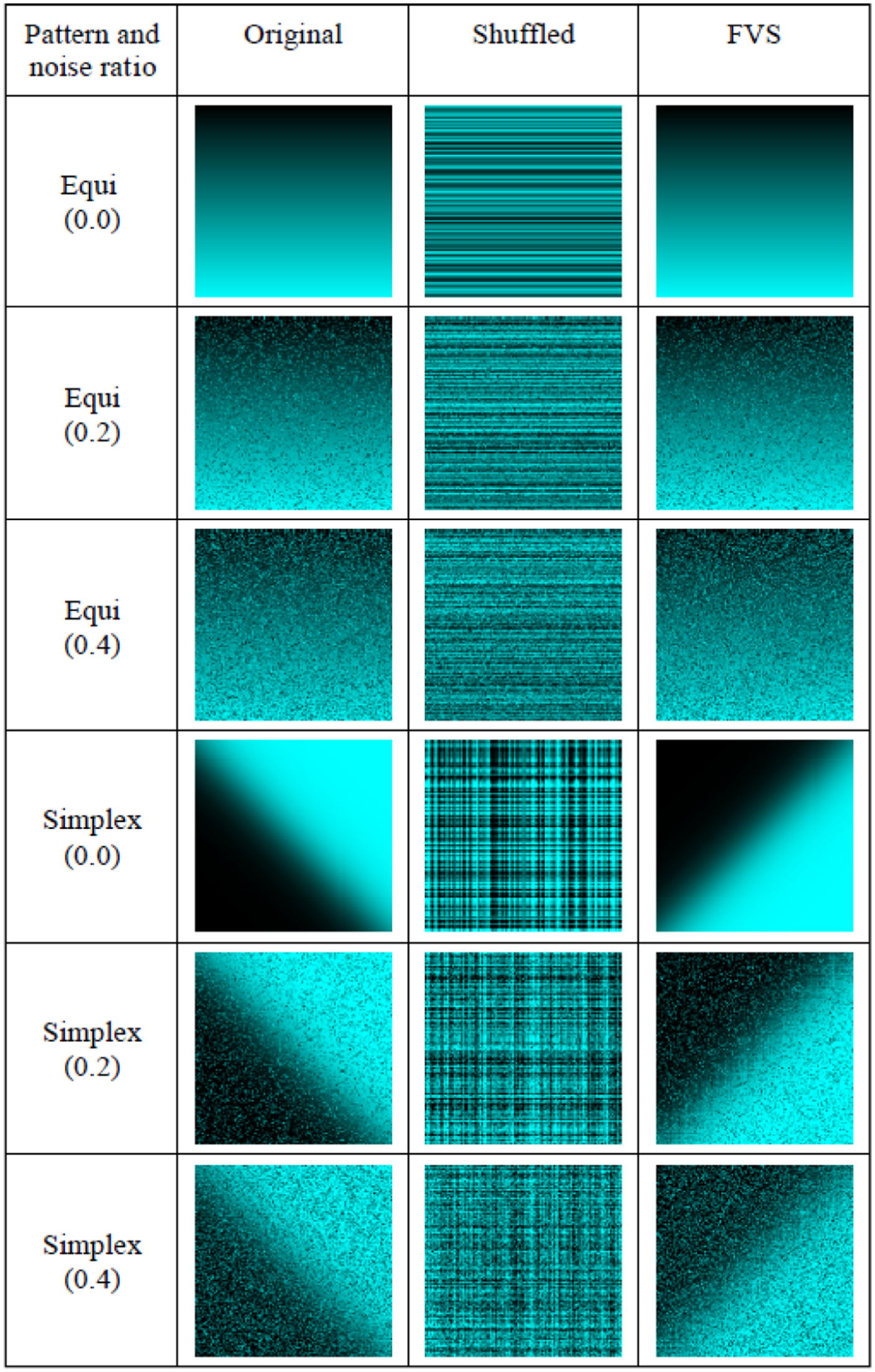
Our experiment also uses shuffling and noising procedures. We use Knuth’s unbiased shuffling algorithm²⁶ for shuffling columns and rows of equi and simplex matrices, in order to provide the pre-equi and pre-simplex matrices used in the experiment. Additionally, our procedure for adding noise to a data matrix was defined as follows.

Given a matrix $M_{m \times n}$ , define its linearized version $M'$ , where $M_{ij}$ and $M'_{in + j}$ are the same cell, $0 \leq i < m$ and $0 \leq j < n$ . Therefore, $| M' | = mn$ .

Define r as the noise ratio, $0 \leq r \leq 1$ .

Create a Boolean array S such that $S_{i} = (i \leq | S | r)$ .

Shuffle S using Knuth’s shuffling algorithm.

For each $0 \leq x < | M' |$ , replace the value of $M'_{x}$ by a random number if $S_{x}$ is true. This random number must be between the maximum and minimum values of M.

The effect of this procedure is salt-and-pepper noise with noise ratio r. Therefore, this noise replaces $u_{ij}$ in our formulation of simplex and equi patterns.

The experiment procedure for each configuration tuple {pattern, parameter b, matrix size, noise ratio, algorithm set} follows.

Create k matrices ${M_{1}, \dots, M_{k}}$ with the predefined pattern, matrix size, noise ratio and parameter b.

Shuffle the rows and columns of these matrices.

For each matrix $M_{i}$ , $1 \leq i \leq k$ , do the following.

Reorder $M_{i}$ with each reordering algorithm from the algorithm set, and measure time spent by each of them.

Measure Moore stress of reordered matrices.

Measure MSLF values of the rows of reordered matrices.

Measure MSLF values of the columns of reordered matrices.

Calculate mean Moore stress for the results of each algorithm.

Calculate mean values of MSLF for rows and for columns of the results of each algorithm.

Calculate mean execution time for each algorithm.

We set $k = 120$ .

Results

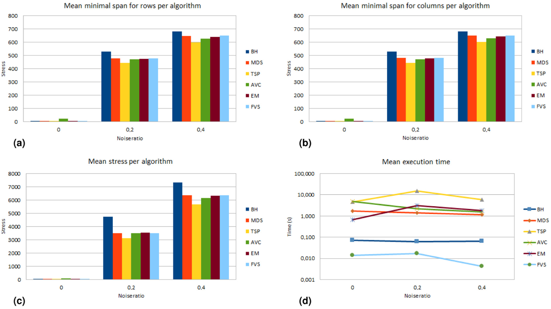
We executed our experiment on 27 parallel processors Power 755 3.3 GHz of an IBM cluster. Figures 4 to 6 and those in Appendix 1 summarize our results. They present mean Moore stress, mean minimal span for rows and for columns, and mean execution time calculated by the MRA tool for our experiment. We will focus our analysis on Figures 4 to 6, related to matrices of size $200 \times 200$ . Similar analysis may be derived from the other six figures in Appendix 1 (Figures 9 –14).

Figure 4.

Experiment results for matrices with pattern simplex ( $b = 0.5$ ) and size $200 \times 200$ . (a) MSLF values for rows. (b) MSLF values for columns. (c) Moore stress. (d) Execution time.

Figure 5.

Experiment results for matrices with pattern simplex ( $b = 1.0$ ) and size $200 \times 200$ . (a) MSLF values for rows. (b) MSLF values for columns. (c) Moore stress. (d) Execution time.

Figure 6.

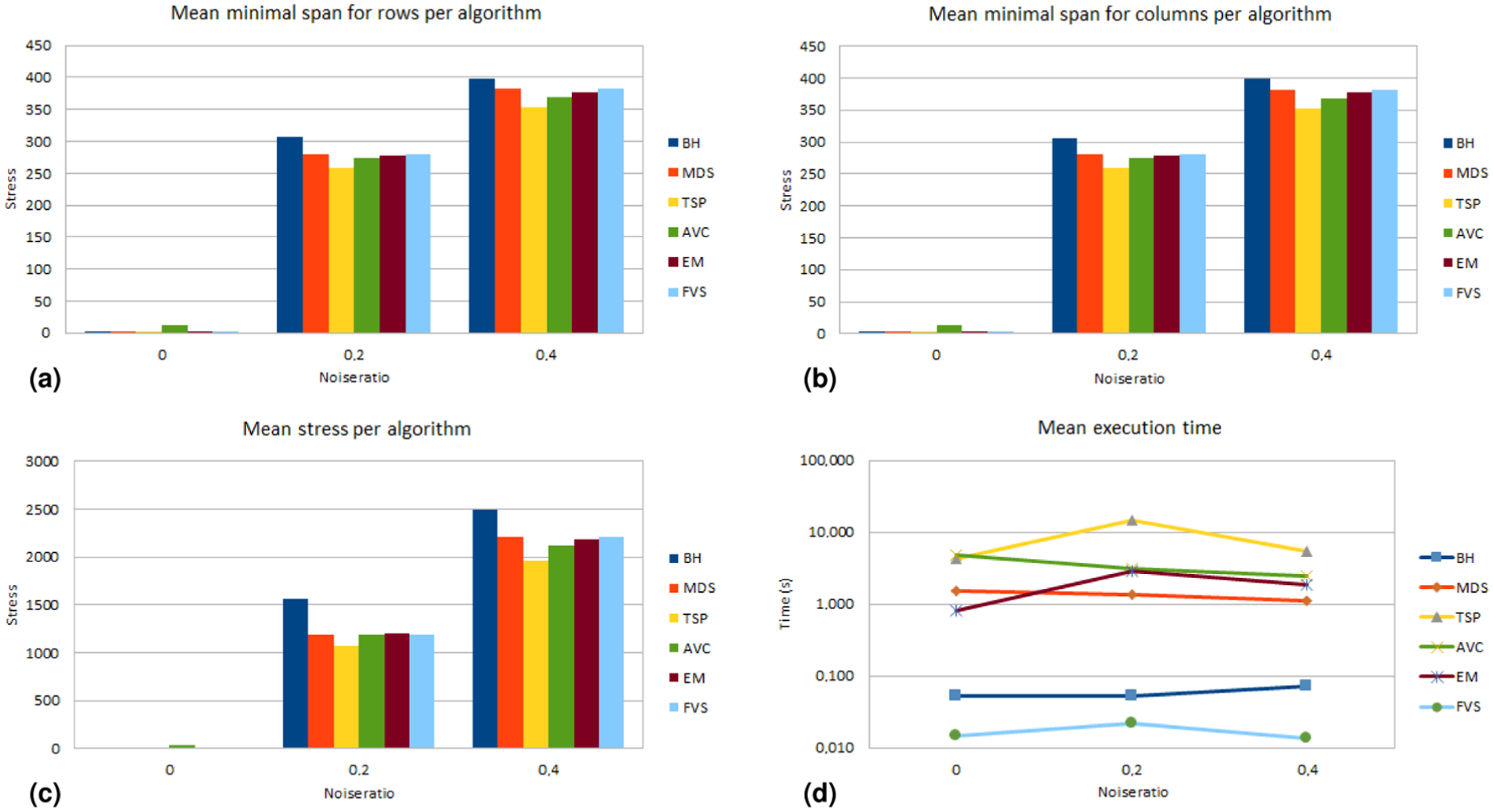
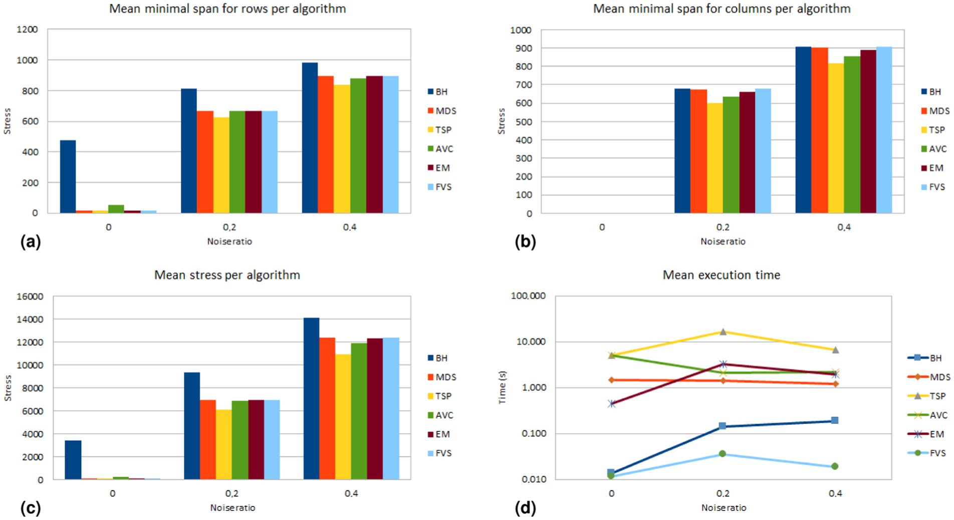
Experiment results for matrices with pattern equi ( $b = 1.0$ ) and size $200 \times 200$ . (a) MSLF values for rows. (b) MSLF values for columns. (c) Moore stress. (d) Execution time.

For the simplex pattern (Figures 4 and 5), mean MSLF values and mean Moore stress for noise ratio 0 are very low for all reordering algorithms. For noise ratios 0.2 and 0.4, we noted that TSP presented the lowest values for these measures, but it was the slowest algorithm. MDS, AVC, EM and FVS produced results with similar mean MSLF values and similar mean Moore stress values. Among them, FVS was the fastest one, with a mean execution time lower than 0.1 s (and in some situations lower than 0.01 s). BH is also a fast algorithm, but its results were the worst ones for these noise ratios.

For the equi pattern (Figure 6), we obtained similar conclusions. It is worth noting that the order of the columns in the equi pattern is less relevant, given the pattern definition.

FVS reached a trade-off between result quality and execution time. It provided permutation results as good as MDS, AVC and EM, but faster, independently of the noise level present in the pre-equi and pre-simplex matrices. We think that these results are generalizable to other noise levels and matrix sizes.

Our approach probably does not apply to other patterns, such as circumplex and band, as we empirically perceived in preliminary tests. Given that other algorithms may produce good results for them, we believe that hybrid methods may be constructed if there is some way to predict which pattern underlies a matrix.

EM (which is based on a TSP solver) returned worse-quality results for these patterns than TSP, despite running faster than it. Also note that AVC may be implemented in faster time complexities than we did in this paper.

Real-world examples

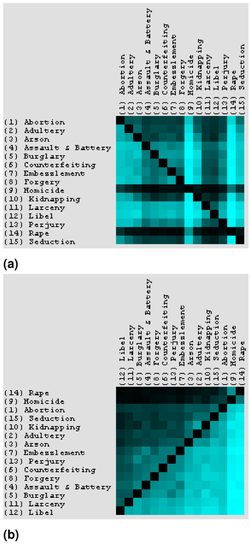
We applied our algorithm to two real-world datasets. Our first dataset was an asymmetric table of pairwise comparisons of crimes and offenses.²⁷Figure 7(a) summarizes the answers of 266 individuals about which crime or offense they consider more serious. In this table, given two crimes $c_{1}$ and $c_{2}$ , a cell ( $c_{1}, c_{2}$ ) (where $c_{1}$ is a row and $c_{2}$ is a column) indicates the proportion of answers “ $c_{2}$ is more serious than $c_{1}$ ”. Cells ( $c, c$ ) have no meaning and have a default value of 0 for any value of c.

Figure 7.

Thurstone’s pairwise comparison about seriousness of crimes and offenses. (a) Original table, as a heatmap. (b) Table reordered by FVS.

We inserted this dataset into MRA and executed FVS, which returned the reordered matrix in Figure 7(b). Note that this matrix is quite similar to a simplex pattern with noise. The analysis of this reordered table reveals an overall continuum among people’s opinions on the seriousness of the analyzed crimes and offenses. It also enables us to conclude that rape, homicide, abortion, seduction and kidnapping were rated as the most serious crimes. In a second scenario, we obtained data from a database of fossil mammals available online at the New and Old Worlds website (NOW public release 030717).²⁸ This database is a spreadsheet with locality of species. We added to this spreadsheet a pivot table whose rows are the species’ order (in a biological sense), columns are countries, and cells count the number of fossils registered at this database. Figure 8 presents how FVS, classical MDS, TSP and AVC reordered this pivot table in MRA. Blue, black and red cells indicate, respectively, low, median and high values. FVS and MDS reveal that this database has a pattern that resembles simplex due to the almost monotonic increasing of values in the vertical and horizontal directions. Both algorithms grouped the highest counts of fossils in a table corner, which was expected for FVS but was not predicted as the behavior of MDS. Both results enable us to perceive that rodents (order Rodentia) and artiodactyls (order Artiodactyla) are well-represented groups of mammals, mainly in Germany, France and Spain. The black and red group of cells forms a cluster of about seven orders of species and covers approximately 24 countries. TSP and AVC split this same group into two or four groups without a clear reason, which seems to hamper matrix analysis.

Figure 8.

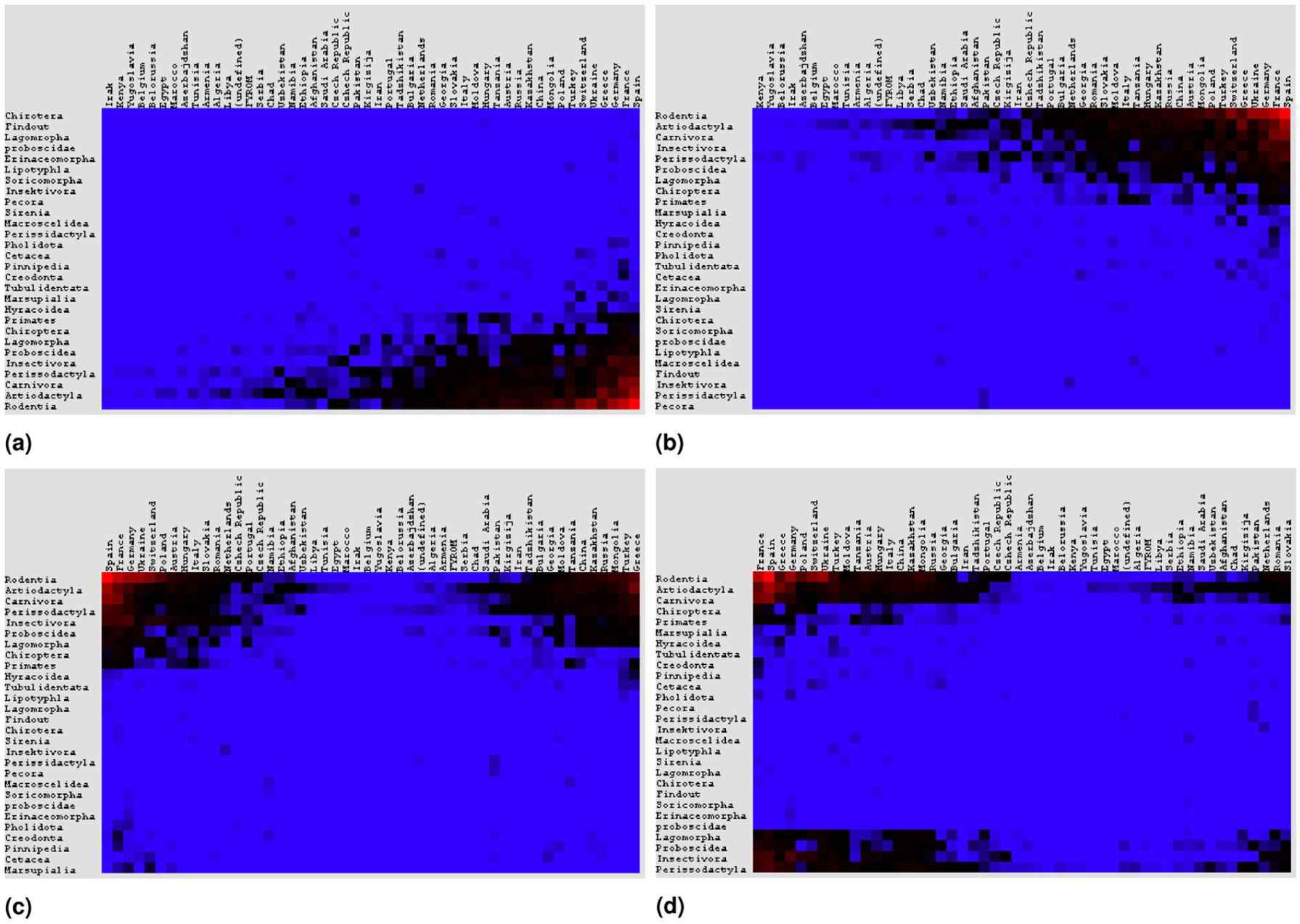
Reordering results for mammal fossil data matrix. (a) FVS results. (b) Classical MDS results. (c) TSP-based algorithm results. (d) AVC results.

Conclusions

We presented our FVS method as a fast ( $O (n^{2})$ ) and easy-to-implement method for reordering matrices without calculating proximity matrices. It was able to reveal simplex and equi patterns on pre-simplex and pre-equi matrices even with a noise level of 40%, and it was executed in much less time than other matrix reordering algorithms. Besides, two real-world examples illustrated that it may produce relevant results. Therefore, it is a competitive algorithm in relation to classical ones (such as classical MDS) for situations in which we know a priori that we have pre-simplex or pre-equi matrices.

Footnotes

Appendix 1 Funding

The author(s) disclosed receipt of the following financial support for the research, authorship and/or publication of this article: This work was supported by the São Paulo Research Foundation (FAPESP) (grant numbers #2014/11186-0, #2015/00411-6 and #2015/14854-7), by National Council for Scientific and Technological Development (CNPq) (grant number 123354/2015-3) and also by CAPES.

References

Bertin

. Semiology of graphics: Diagrams, networks, maps. USA: Esri Press, 2010.

Liiv

Seriation and matrix reordering methods: An historical overview. Stat Anal Data Min ASA Data Sc J 2010; 3(2): 70–91.

Wilkinson

The grammar of graphics. New York, NY: Springer Science & Business Media, 2005.

Gonzalez

Woods

RE.

Digital image processing. 3rd ed.Upper Saddle River, NJ: Pearson/Prentice Hall, 2008.

Tzeng

Chen

. Matrix visualization. In: Chen

Härdle

Unwin

(eds.) Handbook of data visualization. New York, NY: Springer, pp.681–708.

Niermann

Optimizing the ordering of tables with evolutionary computation. Am Stat 2005; 59(1): 41–46.

Mueller

Martin

Lumsdaine

. A comparison of vertex ordering algorithms for large graph visualization. In: Proceedings of the Asia-Pacific symposium on visualisation 2007, Sydney, Australia, 5–7 February, pp.141–148. Danvers, USA: IEEE.

Bezdek

Hathaway

. VAT: A tool for visual assessment of (cluster) tendency. In: Proceedings of the international joint conference on neural networks 2002, Honolulu, Hawaii, 12–17 May 2002, pp.2225–2230. Danvers, USA: IEEE.

DiMaggio

Jr McAllister

Floudas

et al . Biclustering via optimal re-ordering of data matrices in systems biology: Rigorous methods and comparative studies. BMC Bioinform 2008; 9: 458.

10.

Climer

Zhang

. Take a walk and cluster genes: A TSP-based approach to optimal rearrangement clustering. In: Proceedings of the 21th international conference on machine learning 2004, Banff, Alberta, Canada, 4–8 July 2004, pp.363–394. New York, NY: ACM.

11.

Djuric

Vucetic

. Efficient visualization of large-scale data tables through reordering and entropy minimization. In: Proceedings of IEEE 13th international conference on data mining 2013, Dallas, Texas, 7–10 December 2013, pp.121–130. Danvers, USA: IEEE.

12.

Chen

CH.

Generalized association plots: Information visualization via iteratively generated correlation matrices. Stat Sin 2002; 12: 7–29.

13.

Chen

Saad

Dense subgraph extraction with application to community detection. IEEE Trans Knowl Data Eng 2012; 24(7): 1216–1230.

14.

Bar-Joseph

Gifford

Jaakkola

TS.

Fast optimal leaf ordering for hierarchical clustering. Bioinform 2001; 17 Suppl 1: S22–29.

15.

Koren

Harel

A multi-scale algorithm for the linear arrangement problem. In: Kucera

(ed.) Graph-theoretic concepts in computer science. Berlin/Heidelberg: Springer, 2002, pp.296–309.

16.

Brusco

Stahl

Branch-and-bound applications in combinatorial data analysis (Statistics and Computing). New York, NY: Springer, 2005.

17.

Ankerst

Berchtold

Keim

. Similarity clustering of dimensions for an enhanced visualization of multidimensional data. In: Proceedings of the IEEE symposium on information visualization 1998, Research Triangle Park, North Carolina, 19–20 October 1998, pp.52–60. Los Alamitos, California: IEEE.

18.

Mäkinen

Siirtola

Reordering the reorderable matrix as an algorithmic problem. In: Anderson

Cheng

Haarslev

(eds.) Theory and application of diagrams. New York, NY: Springer, 2000, pp.453–468.

19.

Ben-Dor

Chor

Karp

et al . Discovering local structure in gene expression data: The order-preserving submatrix problem. J Comput Bio 2003; 10(3/4): 373–384.

20.

Silva

Melo

Silva

et al . PQR sort: Using PQR trees for binary matrix reorganization. J Brazil Comput Soc 2014; 20(1): 3.

21.

McCormick

Deutsch

Martin

et al . Identification of data structures and relationships by matrix reordering techniques. Technical report, Institute for Defense Analyses, VA, 1969.

22.

Arabie

Hubert

LJ.

The bond energy algorithm revisited. IEEE Trans Syst Man Cybern 1990; 20(1): 268–274.

23.

Torres

Silva

Medeiros

CMB

et al . Visual structures for image browsing. In: Proceedings of the twelfth ACM international conference on information & knowledge management 2003, pp.49–55.

24.

Torgerson

WS.

Multidimensional scaling: I. Theory and method. Psychom 1952; 17(4): 401–419.

25.

Tzeng

HHS

WH.

Multidimensional scaling for large genomic data sets. BMC Bioinform 2008; 9:179.

26.

Knuth

. The art of computer programming. Vol. 2. Reading, MA: Addison-Wesley, 1981.

27.

Thurstone

LL.

The method of paired comparisons for social values. J Abnorm Soc Psych 1927; 21: 384–400.

28.

Fortelius

. New and old worlds database of fossil mammals (NOW), http://www.helsinki.fi/science/now (2003, accessed 20 July 2016).