Graph query algebra and visual proximity rules for biological pathway exploration

Abstract

We present the design and validation of an example-based pathway graph query algebra and visual proximity rules to address challenging large biological pathway exploration tasks. Our pathway graph query algebra interprets relationship queries given by selected examples to find a match for, extract identical parts between, or trace a path from any pathway components. To support the relationship query, users can composite pathway visualizations through visual proximity rules that use proximity to infer users’ intentions in the exploration process. By allowing selection of one or more objects from multiple on-screen grouped graphs as query inputs and using the query outputs as next-query inputs, pathway graph query algebra and visual proximity rules achieve intuitiveness, concurrence, and dynamics for pathway exploration.

Keywords

Biological pathway relational query interactive metaphor visual analytics graph visualization

Introduction

Biological pathways partition biological entities into smaller pieces relevant to individual biological processes. Mathematically, these pathways are compound graphs that contain hierarchical tree structures over network. For example, pathways contain sub-pathways that include cellular locations (compartments) that further contain biomolecules as nodes and biological relationships as edges. In addition to structural network, nodes and edges in these compound graphs also carry numerous semantic attributes, such as gene-expression levels and cross-talk attributes (genes which keep the same function in several pathways). Interpreting such complex relationships is one of the most challenging problems in biological data visualization. If successful, a visualization tool can guide biologists toward the most valuable scientific hypothesis or insights.¹

To design effective visualization tools, scalability becomes a major issue in pathway exploration that has to do primarily with the intricate relationships in large pathways. There are inevitable conflicts among visualization size, limited screen space, and limited human memory. Reducing the complexity of the visualization by partitioning a graph into smaller units can alleviate this conflict. Constructing visualizations in a multi-scale multi-view fashion is another way to improve scalability.² This work combines both approaches and extends the novel metaphor^3,4 to graph exploration by introducing visual proximity rules (VPRs). The metaphor is shown as bubbles, small views that contain a visualization segment. VPRs use view proximity to infer users’ intentions in compositing visualizations and organizing relationships among the visualization segments contained in bubbles.

Pathway graph query algebra (PGQA) is proposed to help biologists explore pathway relationships. It is based on a participatory design and a characterization of the questions asked in pathway analysis. Partly inspired by the database query language Query by Example (QBE),⁵ PGQA lets users make queries by creating examples on the screen. Concurrency is inherent in PGQA since multiple examples can be used in a single query and single queries can be made across multiple pathways at the same time. It may be the first tool of its kind designed for pathway exploration.

The major contributions of this research are (1) a list and analysis of the questions asked in pathway relationship analysis, (2) a PGQA that supports concurrent pathway explorations, (3) VPRs for supporting flexible graph visualization composition and graph exploration, and (4) an exploratory environment for biological pathway studies and use cases demonstrating our approach.

Related work

Pathway relationship exploration

Among the tools used for pathway relationship exploration are many general-purpose graph tools.⁶ Several such tools focus on designing graph layouts or multi-view interactions to facilitate relationship exploration. For example, interconnection between pathways can be visualized in an overall network as used in KEGG Atlas⁷ or can be highlighted by Focus + Context methods in Entourage,⁸ where one pathway map is the focus and is linked to subsets of related pathways. A work similar to ours is enRoute,⁹ which interactively explores experimental data along user-selected paths. ConTour¹⁰ also explores multi-relational datasets for drug discovery through brushing and linking. Complimentary to these powerful tools, our design aims to provide quick relationship discovery through interactive query without making biologists browse through the large and complicated pathways.

QBE

QBE⁵ lets users make queries by creating examples on the screen. Spatial-Query-by-Sketch¹¹ lets the user formulate a spatial query by drawing the desired configuration which is translated into a symbolic representation used to query a geographic database. This work is similar to QBE in using visual examples created on the screen.

Several query languages designed for graph databases use graph structure.¹² Compared to common query languages, our query algebra is semi-structured (impose less strict schemas on input data type and order) and example-based (interactively created by users through mouse clicks and menu selections).

Progressive refinement in multi-view exploration

Biologists’ query is a dynamic process of iterative data reading, comparison, and interpretation. Our approach makes use of a progressive refinement through a multiple view environment to scaffold this query process, which can free biologists from memorizing the dynamic query process, especially when pathway visualizations become bigger than the screen.

Among the efforts in building progressive multi-view visualization, some have studied how to accommodate visualizations and interactions in unified environments based on a metaphorical bubble interface,^3,4 while others explore ways to externalize visible thinking on a whiteboard-style interface¹³ or, similarly, to help users improvise visualizations in coordinated views.^14–16 A successful example that adopted the bubble-based interface for compound graph exploration is PathRings.² We use the key features of a bubble-based interface in VisBubbles⁴ and PathRings,² including flexible view management, continuous virtual workspace, and semantic bubble groups, to support biologists in laying out, navigating, constructing, and querying pathways.

Data characterization and requirement analysis

Data characterization

Biological pathways have complicated relationships within and between them. The within-pathway relationship is usually expressed as a compound graph¹⁷ depicting both interactions between biomolecules and containing relationships between pathway components at three levels: pathway (PW), compartment (CP), and biomolecule (BM). The between-pathway relationship, formed by sharing cross-talk proteins between different pathways, is represented by a link between two shared pathways or cross-talk proteins. In addition, each pathway forms a compound graph since a biological pathway may be broken down into sub-pathways that may be linked to each other through shared nodes (biomolecules), links, or sub-graphs (compartments).⁸Figure 1 shows this type of multiplex network with three types of pathway relationships.

Figure 1.

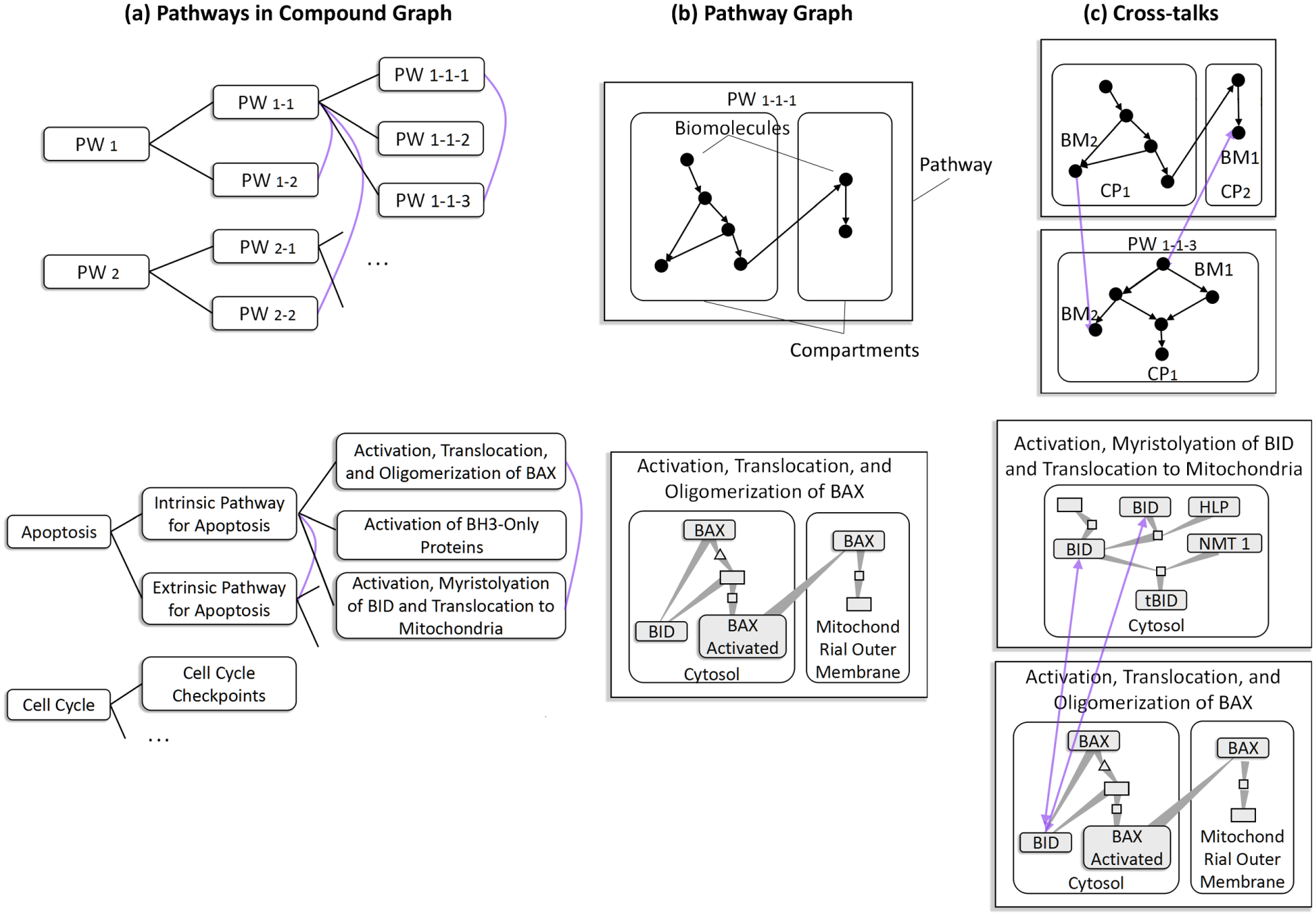
A multiplex network with three types of pathway relationships. Figures on the top row give abstract illustrations; those on the bottom are examples. (a) Pathways in compound graphs. Reactome¹⁸ stores all human pathways in hierarchies in which a lower level pathway describes a subtopic of its parent pathway. The purple curves indicate cross-talk between pathways. The cross-talking pathways share same proteins as shown in (c). (b) Pathway graph. A graph connecting biomolecules within a pathway forms a pathway graph. Three levels are shown: pathway (PW), compartment (CP), and biomolecule (BM). (c) Cross-talks between pathways via cross-talking proteins. For example, the second row shows two pathways cross-talking through a shared cross-talking protein BID.

Pathways in compound graphs

Our pathway representation follows that of Reactome,¹⁸ a public repository of an open-access, manually curated, peer-reviewed pathway database. Reactome organizes hierarchical structures containing about 20–30 top-level pathways, each depicting a biological process under an aggregated topic (e.g. metabolism). Two pathways are considered related (have edge links) when they share biological entities (nodes), share edges, and/or one is contained or referenced in the other.⁸

We use TreeRing^2,19,20 to encode the hierarchical relationship of pathways through ring layers and cross-talks through edges. The example of TreeRing in Figure 2 gives an overview of over 1300 pathways collected from Reactome database.¹⁸ In the tree view, each pathway is rendered as a tree ring node, that is, a ring sector. A ring sector is further segmented into four ribbons color-coded according to the number of cross-talking proteins (proteins that function in multiple pathways), the ratio of differentially expressed proteins to total number of proteins (when linked with input expression), whether the pathway contains rate-limiting proteins (proteins that play important roles in determining the rate of the overall reaction in a multi-step reaction) and orthologous proteins (the “same” proteins in different species sharing a common ancestor protein). The lower level pathways are much simpler and are contained by top-level pathways. Biologists can open the hidden sub-pathways through menu operations.

Figure 2.

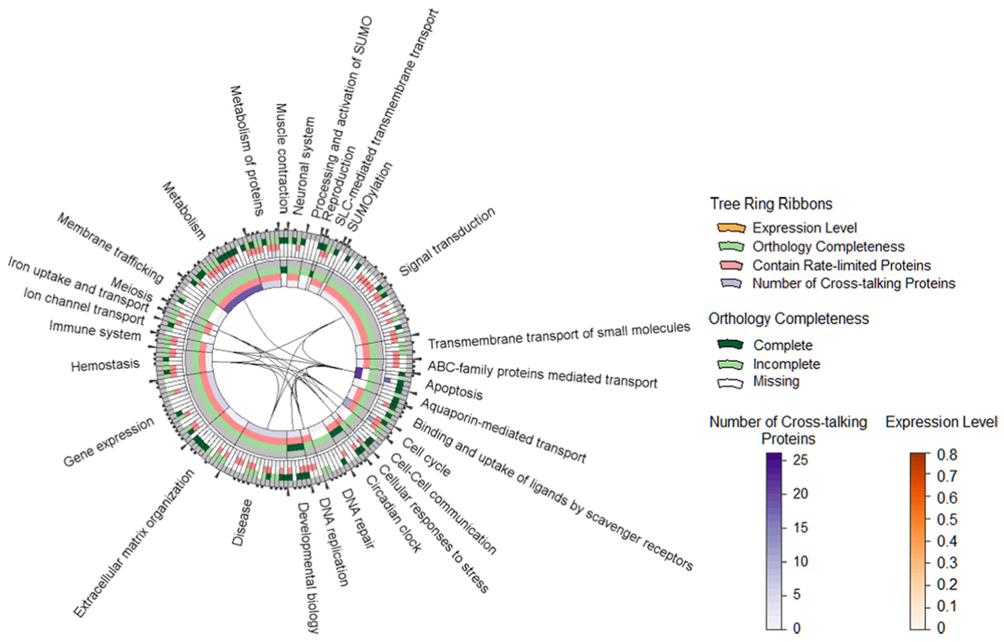
TreeRing: an overview of all Reactome pathways in two layers, each of which contains four concentric circles to encode: (1) the number of cross-talking proteins in a pathway, (2) whether or not a pathway contains rate-limiting proteins, (3) ratio of differentially expressed proteins to the total number of proteins of a pathway, and (4) completeness of orthologous proteins of a pathway (whether all of, part of, or none of its proteins can be found in an given orthologous protein list). Edges indicate that there exist cross-talks which are shared between pathways.

Pathway graph

Interactions between pathway components are represented by graphs. The graph in a pathway consists of nodes presenting biomolecules protein, complex, small molecule, and so on, and directional edges indicating the input, output, or catalyst of the reactions. Nodes are located in cellular compartments inside the pathway.

An example pathway graph is shown in Figure 3. Our graph layout integrates a force-directed algorithm (to reduce edge crossing and edge lengths),²¹ a hierarchical layout (to emphasize compartment information),²² and tapered edges (to emphasize direction).²³ The attribute markers for up-expressed and down-expressed proteins are colored in contrasting red and blue to stand out among a large group of biological entities in analogous yellowish and greenish colors (adjacent colors on the color wheel). Similarly, cross-talking, rate-limited, and orthologous proteins are marked with distinctive colors. The contrasting green and orange are used to highlight the opposite inhibition and activation attributes of edges.

Figure 3.

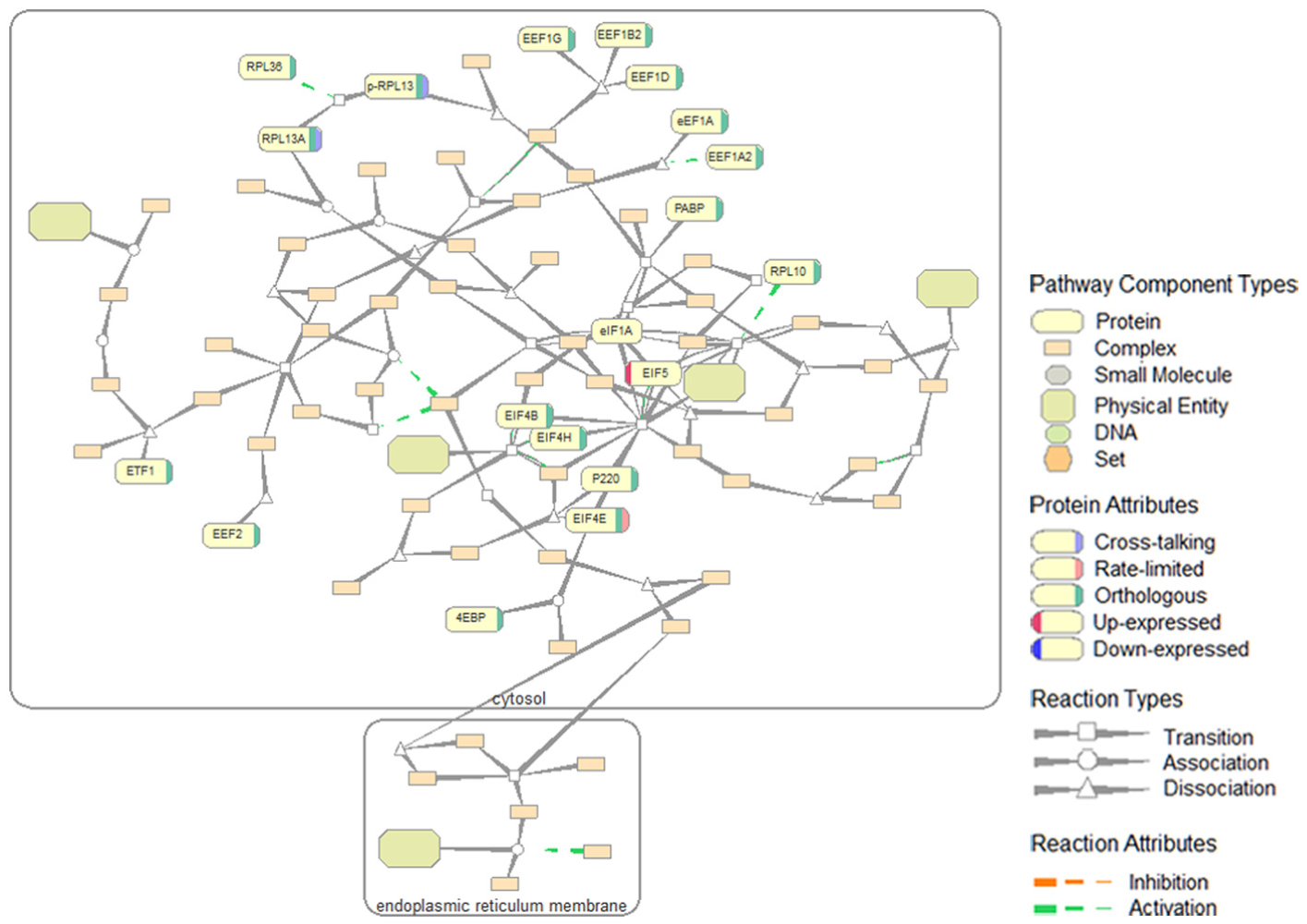
The “Translation” pathway graph and symbols used in pathway graphs.

Cross-talk between pathways

The most common pathway relation is that defined by the so-called cross-talking proteins (Figure 1(c)): changes in one pathway may affect the others carrying the same proteins. Cross-talking proteins are critical in analysis scenarios such as judging effects of drugs in biopharmaceutical research.²⁴ Changes in the expression of such proteins may affect multiple pathways and have significantly more impact on biology than proteins that function in a single pathway.

Analytical tasks

Our design started from observing biologists’ activities of two sorts: study of cross-talks between pathways and gene-expression analysis, which involves exploring both individual pathways and groups of cross-talking pathways. Except for viewing data content (e.g. does a pathway cross-talk? which proteins have high expression levels? how many expressed proteins does a pathway have?), analytical tasks are of three main types: (1) searching interesting pathway components, (2) tracing paths, and (3) comparison (identifying shared parts) between compartments and pathways. For example, biologists may be interested in certain proteins or a path of a protein destined for secretion. Biologists’ queries span different levels (pathways, compartments, and nodes in pathway graphs). They also wish to perform queries based on previous query results or query multiple objects at the same time.

We list in Table 1 six basic-level questions that biologists often ask during pathway exploration and categorize them according to the relationship types they involve and levels of pathway components they cover.

Table 1.

Questions for the analysis of pathway relationships.

Questions		Levels			Relationships	Analytical tasks
		PW	CP	BM	Relationships	Analytical tasks
Q1	Is a protein in other compartments?		X	X	Within-pathway	Match
Q2	Is a protein in other pathways?	X		X	Between-pathway	Match
Q3	Are there any shared proteins in given compartments?		X	X	Within-pathway	Compare
Q4	Are there any shared proteins in given pathways?	X		X	Between-pathway	Compare
Q5	What are the gene products linked to a given protein?			X	Within-pathway	Path tracing
Q6	What are the paths connecting two given proteins?			X	Within-pathway	Path tracing

BM: biomolecules; CP: compartment; PW: pathway.

Design goals

To support biologists’ data exploration and analysis activities above, we have derived the following design goals:

G1: Scalability. It is the main concern in our design due to the size and complexity of the pathway datasets. Allowing exploring pathways in a hierarchical way and extracting and re-composing sub-pathways in multiple views can help achieve data scalability. Visual scalability is further enhanced by allowing overviews, zoom and filter, and details-on-demand (but not necessarily following the order in Shneiderman’s original “overview, zoom and filter, then details-on-command” information-seeking mantra²⁵).

G2: Dynamics. Biologists’ exploratory and analytical processes are dynamic: their exploration path is unpredictable and they often go back and forth between one visualization and another before-making sense of different pathway components. We address dynamics by providing a flexible view manipulation capability for users to create and modify their visualizations.

G3: Synchronization. Path extraction and searching nodes, compartments, and pathways of interest are frequent activities of biologists. Those activities are also highly repetitive and can be synchronized for different pathways.

Progressive exploration environment

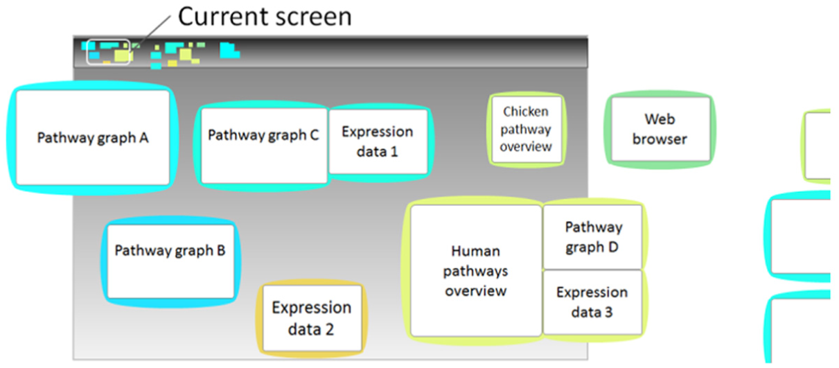
Our visualization environment was iteratively designed in collaboration with the two biologists who are also our target users and coauthors and followed the principles of direct manipulation.²⁶ Direct drag-and-drop enables users to rapidly explore, filter, and select elements from visualizations. Tight coupling allows continuous updating between coordinated views to increase the fluidity of interaction.¹⁴Figure 4 shows the interface and sample visualizations that we build in our visualization environment. Combined with “bubble interfaces”^3,4 which helps users to manipulate views incrementally, it has several features:

Intuitive visualization composition—menu and direct dragging are designed to support operations such as grouping, splitting, ungrouping, and merging different views to composite visualization.

Automatic view management—whenever overlap between bubbles or disconnection between grouped bubbles happens after a bubble is created, moved, rescaled, grouped, ungrouped, or deleted, an automatic spatial-layout algorithm is invoked to incrementally modify bubble locations.

Pannable workspace—a pannable bar shows an overview map of the entire workspace. This makes possible a continuous virtual space, so that biologists need not toggle between the virtual desktops in a classical discrete space.

Synchronized operations—operations applied to one bubble of a group are applied to the others.

Figure 4.

An exploratory multi-view visualization environment: (a) virtual workspace, (b) TreeRing overview of all pathways, (c) pathway Apoptosis, (d) expression data, (e) text search, (f) eGIFT iTerms²⁷ for protein CYCS, (g) compartment nuclear envelope that has been removed, (h) compartment nucleoplasm that has been dragged out from pathway Apoptosis, (i) the drop-down menu that supports file management, view manipulation, and graph query, and (j) legend map of visual encodings. The thick gray edge on the left links the pathway in (c) to its corresponding TreeRing node in (b); the thick gray edge on the right links protein CYCS in (c) to its eGIFT iTerms in (f).

It also provides simple tools such as keyword search for pathways and proteins, remote access to eGIFT (an online database for biologists to query the informative terms, that is, iTerms, mined in literatures containing related gene),²⁷ for biological entities, quick pathway loading by dragging it out of a TreeRing bubble or, for the cross-talking case, opening cross-talking pathways by menu at a cross-talking protein location. Our environment was implemented in Visual Studio C++ and used an open-source software Qt 4.8.

Visual proximity rules

View manipulation through VPRs

In the context of pathway study, we believe, graph visualizations work best when the graphs are put close to each other in multiple views organized so as to reflect their relationships. For example, cross-talking pathways would group together; the pathways or their sub-graphs which are less interested by biologists would be placed at peripheral views around the focused views. In addition, the directness of interaction improves learnability, memorability, expert performance, and so on.²⁸ Dragging a visual object through a short distance is the most common and direct interaction. We therefore introduce VPRs that use proximity to infer users’ intentions in compositing graphs and exploring relationships.

Through VPRs, users can intuitively composite a multi-view visualization to explore pathway data by merging, grouping, splitting, linking, ungrouping, and deleting bubble views that contain a visualization segment. Figure 5 illustrates all the view manipulation cases through VPRs as listed below.

Figure 5.

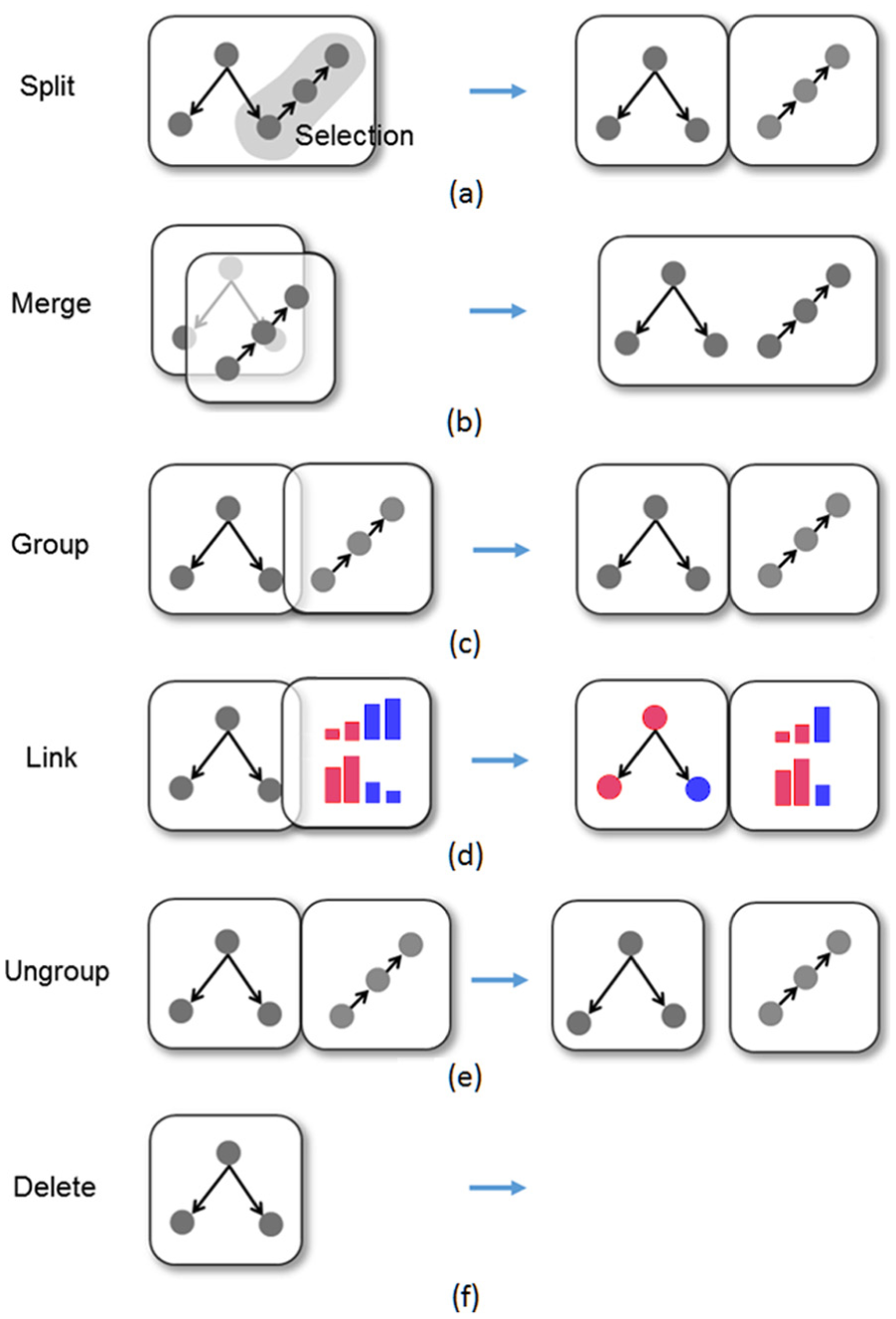
A taxonomy of multi-view composition through visual proximity rules (VPRs).

Split—one view is split into two views which each contain a part of the visualization. Sub-pathway can be constructed using arbitrary shape selection. These two sub-graphs will be in the two separated views (Figure 5(a)).

Merge—two views are merged into one as a user drags one view onto the other when these two views overlap more than half of the size of a single view. The once separate visualizations in two views are fused into one where the common nodes and structures are displayed only once (Figure 5(b)).

Biologists can extract and recombine sub-graphs of a pathway. There are two ways of extracting sub-graphs from a bubble: (1) using a pen (found through menu operations “Tools → Pen Selection”) to circle selected pathway components or (2) directly dragging an item out of a pathway bubble. Drawing a region on the bubble and dragging the selected items to an empty space will open a bubble showing all the components contained in the circled region. Biologists can also drag a single pathway component such as a compartment or a protein out of a bubble. The dragged items will be shown in a new bubble. An example is shown in Figure 6. In addition, biologists can drop a bubble containing a sub-graph back to the bubble to recover the original pathway graph.

Figure 6.

Select a sub-graph in a pathway. Left: after circling a group of nodes. Right: after dragging the selected sub-graph out of the original pathway bubble.

Group/Link—two views are grouped side-by-side as a user drags one view on top of the other (Figure 5(c)). The grouped views of same types respond to the same user inputs. For example, if a bubble of the group is linked to an expression data, a new bubble added to the group is also linked to the same expression data.

The grouped views of different types may trigger a “link” operation. A typical example is that grouping an expression view with a pathway view highlights the up-expressed (meaning the increase in the gene-expression levels, highlighted in red) and down-expressed (meaning the decrease in the gene-expression levels, shown in blue) proteins in a pathway bubble. Meanwhile, in the expression bubble, only the genes expressed in the linked pathway bubble remain visible (Figure 5(d)).

Figure 4 gives an example of grouped expression data and pathways. After a biologist picks an expression data through menu operations “Open → Expression,” the gene-expression data are shown in an expression bubble with bar charts.⁹ Grouping expression bubbles with pathway bubbles automatically highlights the genes in both expression (Figure 4(d)) and pathway (Figure 4(c)) bubbles.

Ungroup—the reverse of group operation (Figure 5(e)). Two grouped views are ungrouped into individual views. Deleting/ungrouping a grouped bubble removes the “link” result between views, for example, the highlighting of the proteins that were expressed according to the expression data, if the view showing the expression data is deleted or ungrouped.

Create/delete—two inverse operations. A default visualization is shown in a newly created view that users can edit later. After deleting a view (Figure 5(f)), the system restores the adjacency of the other views in the group, if a disconnection occurs.

Deleting uninterested bubbles saves space and simplifies visualizations. On the other hand, biologists can also get simplified visualization by deleting a sub-graph by extracting the interested sub-graph into a new bubble and deleting the whole original bubble containing the uninterested parts of the pathway. Figure 4(g) indicates the blank spot for the compartment nuclear envelope that has been removed in this way.

Colors are used to show the types and groups of the views and thus provide a perceptible structure of how the views are organized. Initially, an artist collaborator rendered bubble boundaries in bright categorical colors (light blue, magenta, yellow, etc.) and used a dark background. We use the categorical colors she provided to indicate the bubble types. The colors for bubbles containing a pathway graph are chosen from a spectrum of light blues, while those showing expression data use colors from an orange spectrum. Boundaries of grouped bubbles are assigned the color of the initial bubble of the group and differ slightly from the boundaries of the other bubble groups nearby. Our color scheme is illustrated in Figure 7. The top pannable bar gives an overview of all views with color blocks presenting the types and locations of bubbles or bubble groups in the system.

Figure 7.

View coloring scheme.

Pathway query algebra

PGQA is based on a QBE paradigm.⁵ A biologist makes a query by simply clicking example objects and selecting query type and level via menu; the system automatically interprets the example objects and highlights objects found in pathway graphs. PGQA harvests the benefits of direct manipulation and human’s ability to quickly perceive and interact with visual objects. Simplicity is achieved from the biologists’ perspective by a visual and implicit object relationship presentation; no query languages such as Structured Query Language (SQL) are needed. Users interact with pathway graph through PGQA by simply selecting an example configuration (objects and expected output level). PGQA parses this input and translates it into a graph query.

Basic concepts

Query level

A user selects a query level so that the query will output objects at the given level, which can be biomolecule (BM), compartment (CP), or pathway (PW) and not necessarily the level of example objects selected. Since biologists are mainly interested in proteins, by default, selecting biomolecule level outputs proteins.

Semantic object

A semantic object is defined as a set of pathway components with a containing parent–children relationship. In a query, selecting a set of items with containing relationships implies that the query is to seek items with the same relationships. If more than one object is contained by another object, or vice versa, more than one semantic object is abstracted. Figure 8 shows all the possible semantic objects composed of items of one to three levels; Figure 8(h) shows an example of user input for which more than one semantic object is extracted.

Figure 8.

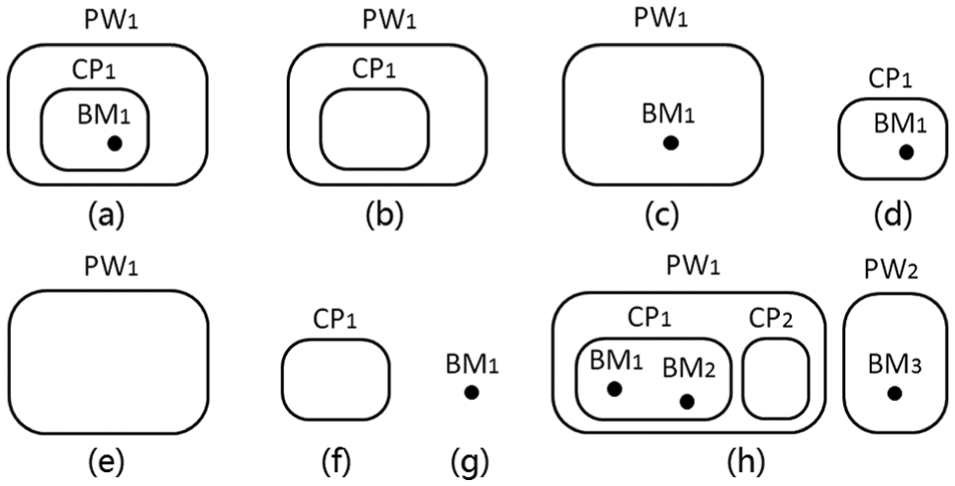
Semantic objects defined by containing relationships: (a) ${ / B M_{1} \in C P_{1} and C P_{1} \in P W_{1}}$ , (b) ${< C P_{1}, P W_{1} > / C P_{1} \in P W_{1}}$ , (c) ${ / B M_{1} \in P W_{1}}$ , (d) ${ / B M_{1} \in C P_{1}}$ , (e) ${P W_{1}}$ , (f) ${C P_{1}}$ , (g) ${B M_{1}}$ , and (h) four semantic objects selected: $Objec t_{1} = { / B M_{1} \in C P_{1} and C P_{1} \in P W_{1}}$ , $Objec t_{2} = { / B M_{2} \in C P_{1} and C P_{1} \in P W_{1}}$ , $Objec t_{3} = {< C P_{2}, P W_{1} > / C P_{2} \in P W_{1}}$ , and $Objec t_{4} = { / B M_{3} \in P W_{2}}$ .

Query algebra

A typical query has three steps: (1) select example objects, (2) set query level, and (3) query (match, compare, or trace path of) each selected object in grouped pathways. Table 2 enumerates all query cases.

Table 2.

Pathway graph query algebra (PGQA).

Input objects	Output level
Input objects	Biomolecule (BM)	Compartment (CP)	Pathway (PW)
(1) Match
BM ₁	All BM₁ proteins	All compartments containing BM₁ (Q1)	All pathways containing BM₁ (Q2)
CP ₁	All proteins in compartment CP₁	All CP₁ compartments	All pathways containing CP₁
PW ₁	All proteins in PW₁	All compartments contained by PW₁	All PW₁ pathways
BM ₁, CP₁ (BM₁∈ CP₁)	All BM₁ proteins contained by compartment CP₁	All CP₁ compartments containing BM₁	All pathways containing CP₁ which contains protein BM₁
BM ₁, PW₁ (BM₁∈ PW₁)	All BM₁ proteins contained by pathway PW₁	All compartments containing BM₁ and contained by PW₁	All PW₁ pathways containing BM₁
CP ₁, PW₁ (CP₁∈ PW₁)	All proteins contained by CP₁ which is contained by PW₁	All CP₁ compartments containing PW₁	All PW₁ pathways containing CP₁
BM ₁, CP₁, PW₁ (BM₁∈ CP₁, CP₁∈ PW₁)	All BM₁ proteins contained by CP₁ which is contained by PW₁	All CP₁ compartments containing BM₁ and contained by PW₁	All PW₁ pathways containing CP₁ which contains protein BM₁
(2) Compare
CP ₁ and CP₂	Shared proteins by compartments CP₁ and CP₂ (Q3)
PW ₁ and PW₂	Shared proteins by pathways PW₁ and PW₂ (Q4)	Shared compartments by pathways PW₁ and PW₂
(3) Path tracing (all paths)
BM ₁	All biomolecules and edges linked to BM₁ in certain reaction steps (Q5)	All compartments and the edges between them linked to BM₁ in certain reaction steps
CP ₁	All biomolecules and edges linked to CP₁ in certain reaction steps	All compartments and the edges between them linked to CP₁ in certain reaction steps
(4) Path tracing (between nodes)
BM ₁ and BM₂	All biomolecules and edges linked to both proteins BM₁ and BM₂ (Q6)
CP ₁ and CP₁		All compartments and the edges linked to both compartments CP₁ and CP₂

Q1–Q6: Question numbers in Table 1 that could be answered by a query.

For example, if users want to find all proteins named SMAD3 contained by compartment Nucleoplasm, they select a SMAD3 and a Nucleoplasm containing it and set the search level to biomolecules (BM). This outputs all SMAD3s contained by Nucleoplasms in the grouped pathway graphs. If the user select the same input but sets the search level to compartment (CP), the output will instead be all Nucleoplasms containing SMAD3 in the group.

Matching

The outputs are the items matching the names and relationships implied by the input sample semantic object. Table 2(1) gives all the input and output cases of a search for the items matched by a single semantic object. If a user selects more than one semantic object, the output is the union of the results of individual input objects: for example, $Match (Objec t_{1}, Objec t_{2}, \dots, Objec t_{n}, Level) = Match (Objec t_{1}, Level) \cup Match (Objec t_{2}, Level) \dots \cup Match (Objec t_{n}, Level)$ .

Comparison

Comparison is made between two compartments or pathways to find all the items they share. Different comparison cases are shown in Table 2(2); example objects must be in the same level and be compartment (CP) or pathway (PW). If more than one semantic object is selected, the output will be the intersection of the results of comparing every two input objects: for example, $Compare (Objec t_{1}, Objec t_{2}, \dots, Objec t_{n}, Level) = Compare (Objec t_{1}, Objec, Level) \cap \dots Compare (Objec t_{1}, Objec t_{n}, Level) \dots \cap Compare (Objec t_{n}, Objec t_{1}, Level) \cap \dots Compare (Objec t_{n}, Objec t_{(n - 1)}, Level)$ .

Path tracing

There are two path-tracing types: one finds paths from the selected objects, the other finds paths connecting selected objects. The two cases are shown in Table 2(3) and (4). If more than one semantic object is selected, the output in the first case will be the union of the results for individual input objects, and in the second case, the union of the paths connecting every input object.

As shown in Table 2, PGQA can actually answer more than the six questions listed in Table 1, giving biologists the potential to explore larger problem domains in various scenarios.

Examples

Query nodes of interest

Biologists input example objects by direct click and find matched or shared items of the selected objects across pathways through menu operations before a query.

Figure 9 shows two typical query results. The items the biologists select as input are highlighted in solid orange boundaries, output items are highlighted with orange halos and each pair of matched items are linked with blue lines. Figure 9(a) shows the results for finding all proteins named SMAD7 contained by compartment Nucleoplasm through menu operations “Selection → Match.”Figure 9(b) shows all the proteins shared by the two pathways through menu operations “Selection → Compare.” The selection of output level is done through menu operations “Selection → Settings.”

Figure 9.

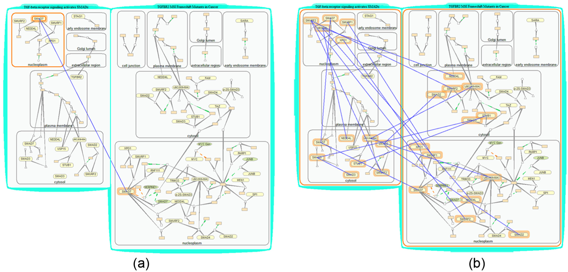
Find items of interest. (a) Search protein SMAD7 that is located in compartment Nucleoplasm. (b) Search shared proteins by two pathways. The input sample objects are highlighted with solid orange boundaries, and objects found are highlighted with orange halos. Pairs of matched items are linked with blue lines.

Query paths of interest

PGQA provides two path-tracing operations. (1) Search “all paths” from a given starting node: highlights all edges and nodes connected with the node in certain reaction steps. Applying this operation through menu operations “Selection → Link → All Paths” successively traces through all paths reachable from the selected node set. (2) Search “linking paths” between selected nodes through menu operations “Selection → Link → Between Nodes.”

Some resulting paths are shown in Figure 10. Figure 10(a) shows the result for finding all paths connected to a complex in three reaction steps. Figure 10(b) shows the result for finding all paths from a compartment. Figure 10(c) shows the path linking two proteins TGFBR2 and SMURF2. Figure 10(d) shows the paths found after a path search for TGFBR2, SMURF2, and a complex.

Figure 10.

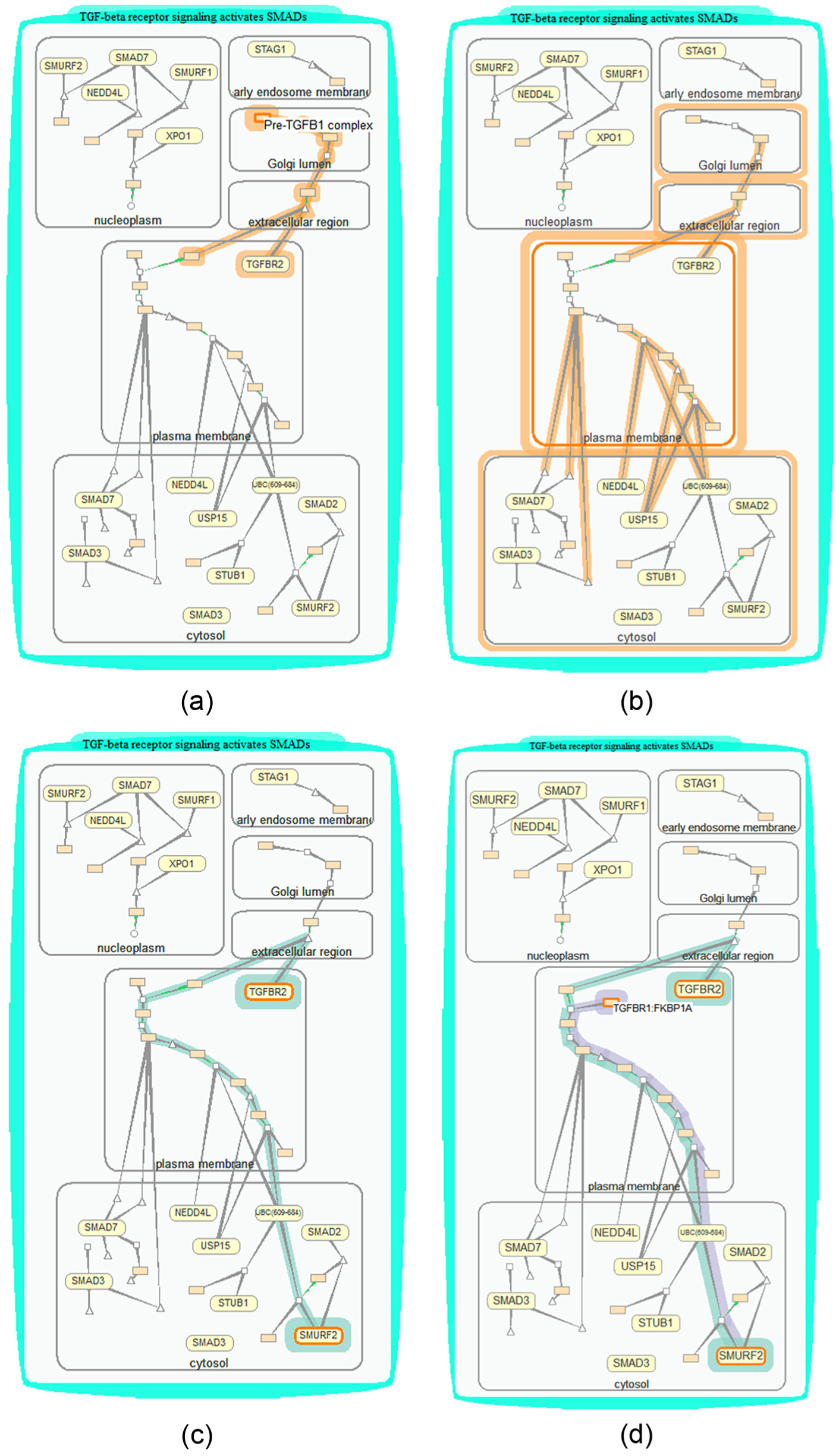
Find paths of interest. The input objects are highlighted with solid orange boundaries and objects found are highlighted with orange halos. (a) Search all paths in biomolecule level linked to complex pre-TGFB1 complex in three reaction steps. (b) Search all paths in compartment level linked to compartment Plasma Membrane. (c) Search paths linking proteins TGFBR2 and SMURF2. (d) Search paths from proteins TGFBR2 and a complex TGFBR1:FKBP1A to SMURF2. The resulted two paths are highlighted in two colors, respectively.

Use cases and discussion

Studying cross-talks between pathways

TreeRing bubbles provide a quick overview for biologists to spot interesting pathways such as those with the most cross-talking, rate-limiting, or up-expressed proteins. Pathway Apoptosis regulates cell death process, making it critical in disease and drug study. Looking at a TreeRing bubble, we find that Apoptosis is marked in dark purple, which means it cross-talks to more pathways than most other pathways. Interested in learning how it cross-talks to others, we open pathway Apoptosis by dragging its corresponding node out of the TreeRing bubble. We find several cross-talking proteins highlighted in purple, for example, protein CYCS. We then open all the pathways containing CYCS through menu operations “Open → Cross-talk Pathways.” These pathways are grouped automatically, and we remove a few pathways or compartments not of current interest to simplify the visualization. We then use the “match” operation to highlight all cross-talks through CYCS among the grouped pathways. Eventually, we are able to thoroughly check all cases of cross-talk in the pathway Apoptosis and learn the possible impacts of the cross-talking proteins over these interrelated pathways. A screen shot of the visualizations built is shown in Figure 11. This usage scenario demonstrates that our tools could help biologists quickly find and inspect cross-talks among large number of pathways.

Figure 11.

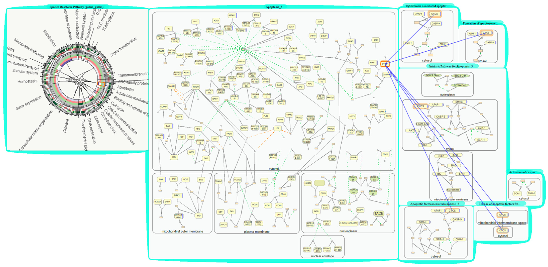
Studying cross-talk between pathways (a bubble group with pathways cross-talking through CYCS).

Studying downstream effect across pathways

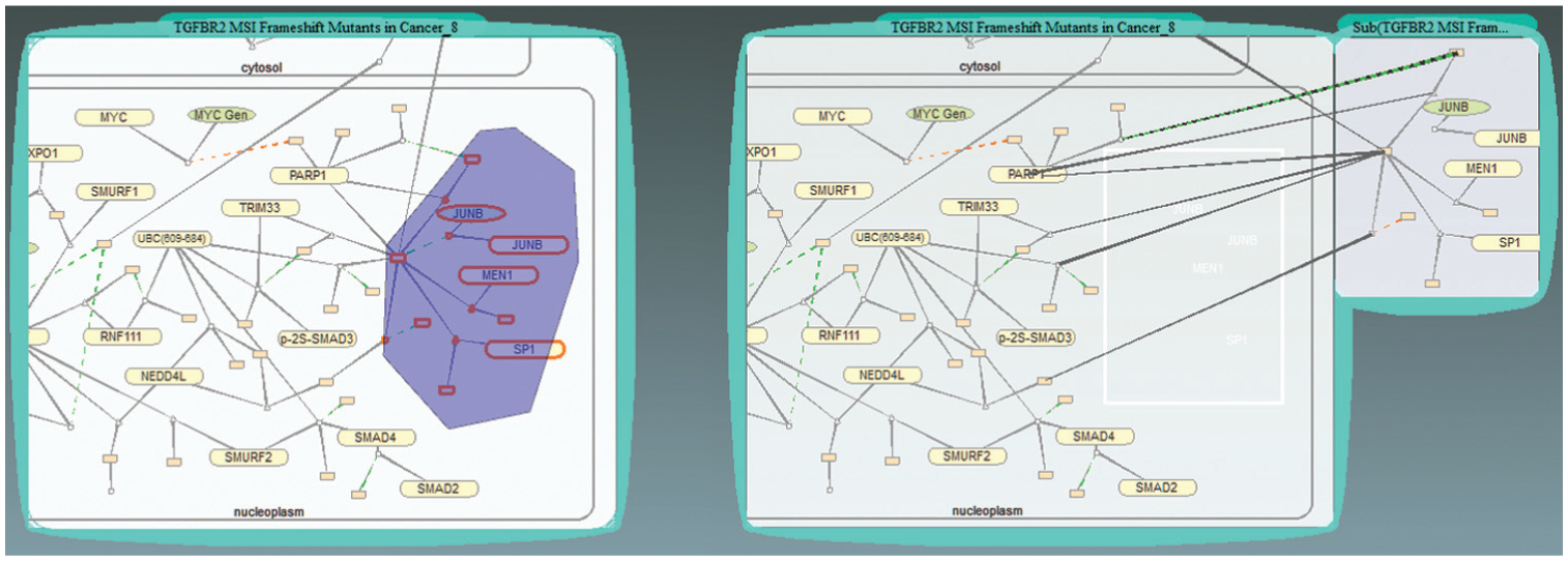
Biologists obtain gene transcriptome data by biological experiments.²⁹ One of the biologists’ primary interests is in transforming growth factor beta (TGF-β) signaling pathways, which are involved in many cellular processes. They load their expression data and group them with one of the transforming growth factor (TGF) pathways TGFBR2 MSI Frameshift Mutants in Cancer. This pathway describes a process in which the TGFBR2 gene is frequently targeted by loss-of-function frame shift mutations in colon cancers with microsatellite instability (MSI). Gene SMAD4 and SMAD7 are found up-expressed (marked in red in Figure 12). SMAD4 and SMAD7 belong to the SMAD family of signal transduction proteins that are essential in forming several protein complexes in TGF-β signaling pathways. Interested in the effect of knocking down gene SMAD4, we use path-tracing operations to highlight all genes connecting with SMAD4. Quickly browsing through the highlighted downstream paths, we find one path leading to protein complex p-2S-SMAD2/3:SMAD4 that will either directly or indirectly regulate the expression of gene MYC, JUNB, and so on inside the nucleus (nucleoplasm).

Figure 12.

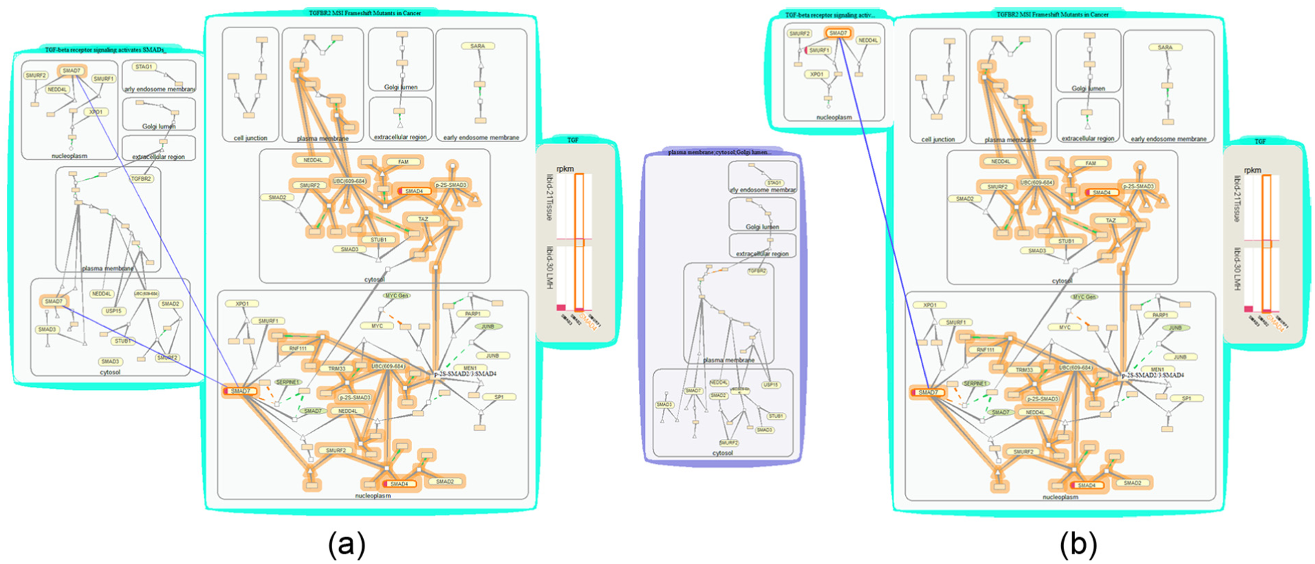
Studying downstream effect of expressed proteins and cross-talk in two TGF pathways: (a) Visualizations built after tracing through the paths from SMAD4 and identifying cross-talks between the two TGF-related pathways. (b) Visualizations built after separating the less interesting parts of a pathway.

To look further at the downstream impact of other TGF-β signaling pathways, we open a related pathway that activates a TGF-β receptor signaling cascade, TGF-β receptor signaling activates SMADs, group the two pathway bubbles, and use the “match” option to find all matched proteins contained by a nucleus in the new pathway for those in the highlighted paths. We find SMAD7 among the shared proteins. Eventually, through PGQA, we learn that knocking down gene SMAD4 will affect the final expression of downstream genes in the cell nucleus and knocking down gene SMAD7 would also affect pathway TGF-β receptor signaling activates SMADs.

The visualizations built during this use case are shown in Figure 12. This use case study demonstrates the usefulness of PGQA and VPRs in identifying downstream effects of a differentially expressed gene based on expression data and in close inspection of cross-talk cases.

Discussion

Our biologist collaborators and coauthors valued the exploratory capabilities of PGQA and VPRs and also found that, with PGQA and VPRs, query became more efficient. The rich interactions provided by our visualization environment were not only easy to use but also addressed their needs effectively in viewing, searching, and compositing new pathway graphs.

We summarize the user experience of the two biologists as follows. (1) Scalability: overviewing complete Reactome pathways and drilling down to small segments such as a single compartment or a few nodes of a pathway at the same time effectively make pathway visualizations scalable. Moreover, all views, large or small, are easily accessible such that all exploration steps can be retrieved. (2) Progressive exploration: VPRs and our visualization environment support a progressive exploration and analysis to address their dynamic exploration workflow. There is a flexibility of switching among different views and placing visualization anywhere and anytime. Even during a random exploration, any information found is recorded in the visualizations, highlighting, and edges linking between views, freeing the biologists from memorizing the scene. (3) Synchronization: performing synchronized query for shared or linked items were exciting time-saving functions rarely found in typical pathway explorers. They can open multiple-related bubbles all at once, rather than having to find and open them one by one as in many other databases or systems. (4) Intuitiveness: the interaction designs, including requesting a query by directly selecting an on-screen example, creating sub-graphs by direct dragging, and conducting synchronous operations among grouped pathway are intuitive and reduce the mental workload remarkably.

We can further improve on our visualization and tool. For example, the graph layout approach can be optimized in terms of minimizing edge crossings by adjusting the stopping condition of the force-directed algorithm and reducing the edge crossings between compartments. Current PGQA augmented with species level may be used to study pathways for different species and answer more comprehensive questions such as integrating data found in specific ontologies to infer signaling and metabolic pathways.

Although our VPR and PGQA are motivated and designed for biological pathway exploration, they can be useful in other graph applications such as social network, brain network studies, or any other large graph applications involving searching similar and different entities.

Conclusion

This article presents a novel solution, PGQA paired with VPRs, to support biologists in interactive pivoting of biological pathways of intricate relationships. As demonstrated, PGQA and VPRs enable dynamic and concurrent queries on different pathway components and thus offer biologists new capabilities and experiences that other tools may not.

Overall, data exploration supported by PGQA and VPRs is an attractive approach to tackling the challenge of big data with complex structures. First, it may well be possible to generalize the synchronized operations allowed among grouped entities through VPRs and relationship exploration through PGQA to any other large graphs and networks. Second, PGQA and VPRs can also be used in other applications to support information-seeking and multi-view explorations. Finally, the initial success of our study in pathway exploration also suggests a new progressive exploration design concept by using proximity to guide view manipulation and directly using examples of visual elements to imply input relations for queries.

Footnotes

Funding

The author(s) disclosed receipt of the following financial support for the research, authorship, and/or publication of this article: This work was supported in part by grants from NSF DBI-1260795, DBI-1147029, and IIS1302755. Any opinions, findings, and conclusions or recommendations expressed in this material are those of the authors and do not necessarily reflect the views of the National Science Foundation.

References

Gehlenborg

O’Donoghue

Baliga

. Visualization of omics data for systems biology. Nat Methods 2010; 7: 56–68.

Zhu

Liang

Alexander

. PathRings: a web-based tool for exploration of ortholog and expression data in biological pathways. BMC Bioinformatics 2015; 16: 165.

Bragdon

Zeleznik

Reiss

. Code bubbles: a working set-based interface for code understanding and maintenance. In: Proceedings of the SIGCHI conference on human factors in computing systems, Atlanta, GA, 10–15 April 2010, pp. 2503–2512. New York: ACM.

Bragdon

Pan

. VisBubbles: a workflow-driven framework for scientific data analysis of time-varying biological datasets. In: Proceedings of the SIGGRAPH Asia posters, Hong Kong, 12–15 December 2011.

Zloof

. Query by example. In: AFIPS ‘75 Proceedings of national computer conference and exposition, Anaheim, CA, 19–22 May 1975, pp. 431–438. New York: ACM.

Munzner

. Interactive visualization of large graphs and networks. PhD Thesis, Stanford University, Stanford, CA, 2000.

Kanehisa

Goto

Sato

. KEGG for integration and interpretation of large-scale molecular data sets. Nucleic Acids Res 2012; 40: D109–D114.

Lex

Partl

Kalkofen

. Entourage: visualizing relationships between biological pathways using contextual subsets. IEEE Trans Vis Comput Graph 2013; 19: 2536–2545.

Partl

Lex

Streit

. enRoute: dynamic path extraction from biological pathway maps for in-depth experimental data analysis. In: Proceedings of the IEEE symposium on biological data visualization (BioVis’12), Seattle, WA, 14–15 October 2012, pp. 107–114. IEEE.

10.

Partl

Lex

Streit

. ConTour: data-driven exploration of multi-relational datasets for drug discovery. IEEE Trans Vis Comput Graph 2014; 20: 1883–1892.

11.

Egenhofer

. Query processing in spatial-query-by-sketch. J Vis Lang Comput 1997; 8: 403–424.

12.

Wood

. Query languages for graph databases. ACM SIGMOD Rec 2012; 41: 50–60.

13.

Walny

Carpendale

Riche

. Visual thinking in action: visualizations as used on whiteboards. IEEE Trans Vis Comput Graph 2011; 17: 2508–2517.

14.

Weaver

. Improvise: a user interface for interactive construction of highly-coordinated visualizations. University of Wisconsin–Madison, Madison, WI, 2006.

15.

Al-Awami

Beyer

Haehn

. NeuroBlocks—visual tracking of segmentation and proofreading for large connectomics projects. IEEE Trans Vis Comput Graph 2016; 22: 738–746.

16.

Streit

Lex

Gratzl

. Guided visual exploration of genomic stratifications in cancer. Nat Methods 2014; 11: 884–885.

17.

Von Landesberger

Kuijper

Schreck

. Visual analysis of large graphs: state-of-the-art and future research challenges. Comput Graph Forum 2011; 30: 1719–1749.

18.

Croft

O’Kelly

. Reactome: a database of reactions, pathways and biological processes. Nucleic Acids Res 2011; 39: D691–D697.

19.

Holten

. Hierarchical edge bundles: visualization of adjacency relations in hierarchical data. IEEE Trans Vis Comput Graph 2006; 12: 741–748.

20.

Zhu

Chen

. EINVis: a visualization tool for analyzing and exploring genetic interactions in large-scale association studies. Genet Epidemiol 2013; 37: 675–685.

21.

Dogrusoz

Giral

Cetintas

. A compound graph layout algorithm for biological pathways. In: Pach

(ed.) Graph drawing. Berlin, Heidelberg: Springer, 2005, pp. 442–447.

22.

Sugiyama

Tagawa

Toda

. Methods for visual understanding of hierarchical system structures. IEEE Trans Syst Man Cybern 1981; 11: 109–125.

23.

Holten

Van Wijk

. A user study on visualizing directed edges in graphs. In: Proceedings of the SIGCHI conference on human factors in computing systems, Boston, MA, 4–9 April 2009, pp. 2299–2308. New York: ACM.

24.

Ashburn

Thor

. Drug repositioning: identifying and developing new uses for existing drugs. Nat Rev Drug Discov 2004; 3: 673–683.

25.

Shneiderman

. The eyes have it: a task by data type taxonomy for information visualizations. In: Proceedings of the IEEE symposium on visual languages, Boulder, CO, 3–6 September 1996, pp. 336–343. New York: IEEE.

26.

Shneiderman

. Direct manipulation: a step beyond programming languages. Comput 1983; 16: 57–69.

27.

Tudor

Schmidt

Vijay-Shanker

. eGIFT: mining gene information from the literature. BMC Bioinformatics 2010; 11: 1–11.

28.

Frohlich

. Direct manipulation and other lessons. In: Helander

Landauer

Prabhu

(eds) Handbook of human-computer interaction. Amsterdam: Elsevier, 1997, pp. 463–488.

29.

Liang

Lamont

Cooksey

. Transcriptome response to heat stress in a chicken hepatocellular carcinoma cell line. Cell Stress Chaperones 2015; 20: 939–950.