Visualizing the strategic landscape of arbitrary games

Abstract

We present Gamalyzer, a game-independent and efficient visualization of sets of play traces. Unlike previous work on game-independent visualization, we focus on sequences of game actions as opposed to sequences of game states. Action sequences directly represent players’ strategic decisions. Moreover, since game actions may already be recorded as part of games’ telemetry and metrics, Gamalyzer is easier to integrate into existing analysis toolchains than state-sequence-based visualizations. Gamalyzer displays each play trace as a vertical line, with symbols along the line indicating game events. Similar play traces (according to the Gamalyzer metric, a specialization of edit distance) are arranged together along the horizontal axis, and as traces become more and less similar to each other over time, they bend towards and away from each other. The Gamalyzer metric is also used to present only the most interestingly different traces in the visualization, with the rest grouped together under their most similar cousins. We position Gamalyzer as an ideal trace filtering and selection tool to be used in concert with a state-centric (and possibly game-specific) visualization for context. This article also provides a detailed account of the Gamalyzer metric and new advice for defining game action schema to maximize the benefits obtained from the tool, along with two detailed case studies of the Gamalyzer visualization in practice.

Keywords

Event analysis play trace visualization game analytics exploratory visualization edit distance

Introduction

What is the purpose of game visualization? Visualization designers assume that mapping quantitative data onto a visual representation helps explain phenomena of interest, or supports insights that could not be as readily obtained by examining the raw data. In devising any new visualization, we have to consider who is expected to use it, what data it uses as input, what phenomena it attempts to present, and, of course, how to treat and display the data. In this work, we assume that the game designer or professional analyst is the target audience.

When we visualize games, specifically gameplay, we have to consider visualization early on in the analytics pipeline. Data-gathering must be incorporated into the game program, testing, and network protocols, and these data must either be useful on their own or they must be sufficient to reconstruct the object of our future analysis. Games have a lot in common with each other, but nearly every game is one-of-a-kind in terms of what data comprise a game state or what game actions can be performed during play. Since the data-gathering process is already so labor-intensive, we hope to develop generic visualizations that can leverage that effort without putting undue constraints on the shape or type of data being collected and without requiring extensive training on the part of the analyst.

Gameplay data are rich and highly heterogeneous along two main axes. First, the subject of the data may be either the events that transpire in the game or the state of the game at various points in time (the difference between textual chess notation and photographs of chessboards). While state data are easy to examine individually, event data are highly contextual; at the same time, event data more directly describe player activity and generalize better across distinct game situations. Second, the data may be fine grained and low level (e.g. individual moves in chess) or it may be more aggregated and abstracted (e.g. the number of pieces captured by each side during a complete game). On the one hand, low-level, concrete instances are simple to understand and relate to real play; but on the other hand, the analyst may miss overall details in a confusion of specific cases.

Our visualization, Gamalyzer¹ (see Figure 1), aims to describe a game’s strategy space: the distinct families of interrelated policies players adopt during play. Since strategies describe the actions players take over time,² we work with sequences of game actions (player inputs) called play traces. Actions are also less expensive to record, store, and transmit than complete captures of game states over time. Importantly, actions may be easier to compare against each other than complete states, especially if some relevant state-related context is provided as part of the action definition. Some questions that we can more readily answer with action sequences than state sequences (and, indeed, with sequences rather than instants or complete aggregates) include the following:

“Do players pursue diverse strategies?”

“Are winning traces similar to each other?”

“What are the outlier plays of this game?”

“Is it possible to win without being at all similar to this canonical trace?”

“How many other players acted mostly like this player?”

“What are the typical solutions to this level? How do players figure out those solutions?”

Figure 1.

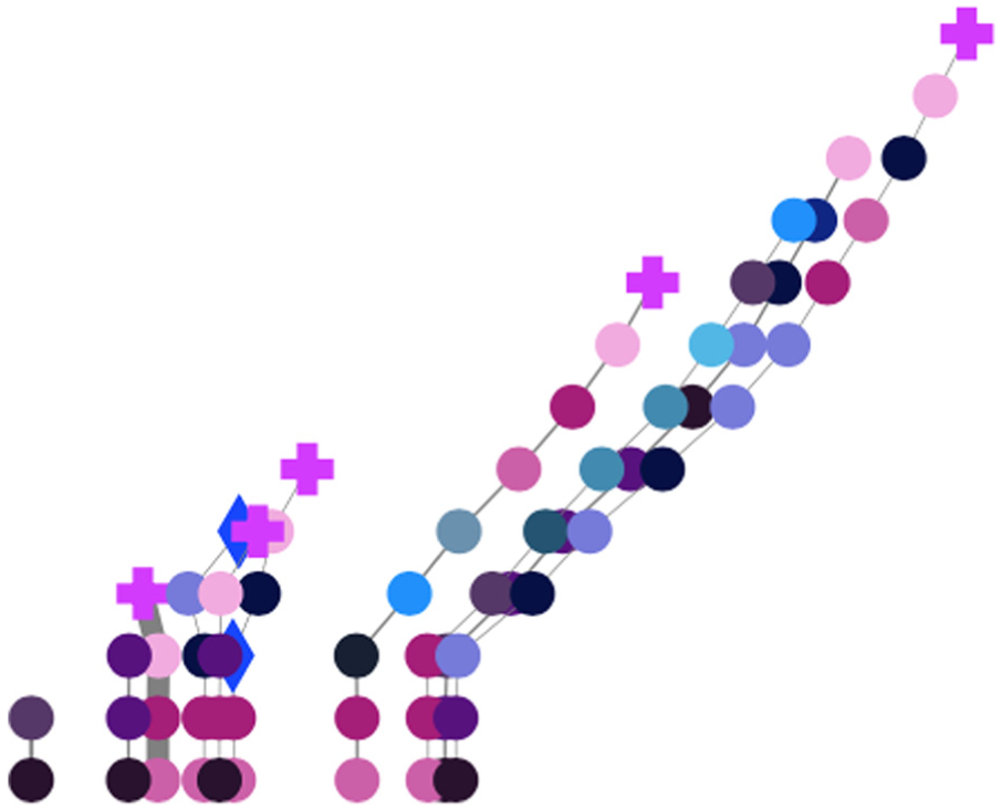
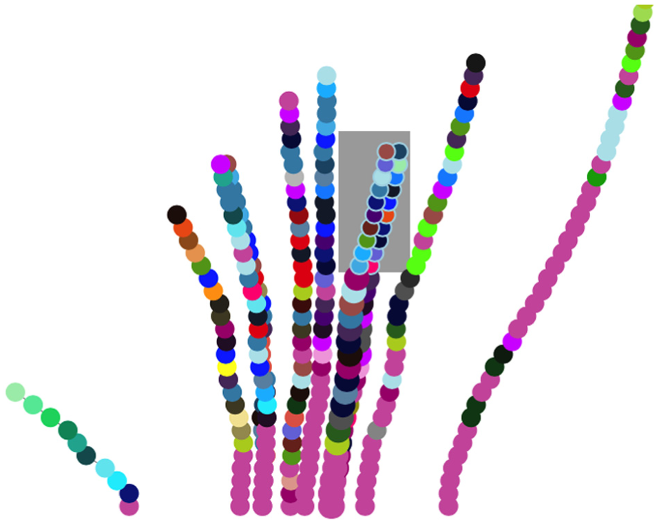
Gamalyzer applied to play traces from the puzzle game Refraction. Each trace is a polyline beginning at the bottom, each input is a colored glyph, and similar traces are grouped together.

These questions suggest four requirements that Gamalyzer must fulfill. First, Gamalyzer must not require the game’s rules as input: it should work only on sets of play traces, without any additional modeling effort. Second, Gamalyzer should cluster together similar play traces for easy appraisal and selection. Third, designers and analysts should not be expected to author similarity measures, distance metrics, layout constraints, or other low-level Gamalyzer-specific features. Finally, the tool must scale well in the number and the length of considered play traces, both in terms of computational efficiency and visual complexity.

Previous work introduced a suitable play trace dissimilarity measure also called Gamalyzer.¹ The Gamalyzer metric is based on the constraint continuous edit distance (CCED),³ a syntactic measure of similarity by which whole play traces (action sequences) are compared against each other. The end result is a number between 0 (identical) and 1 (incomparably different), though a matrix of incremental differences is generated as a side effect. Importantly, analysts may opt to either define an action-versus-action dissimilarity metric or use the default metric, a weighted lexicographic order over actions’ parameters. Initially, Gamalyzer was evaluated automatically against a synthetic dataset and against previous efforts in player model identification. It has since been validated against human designers’ perceptions of play trace difference⁴ and versus non-designer perceptions of human-like play style.⁵ In sum, Gamalyzer has been used with four distinct games (one real-time game, one short puzzle game, and two longer puzzle games) and integrated into two game engines (gathering and visualizing play traces from a puzzle game maker and a real-time 3D game engine), though its performance in one of the longer puzzle games and in the two game engines has not been evaluated.

This article introduces the Gamalyzer visualization, expands on the definition and use of the metric for an audience which may not have seen it before, and relates it to other recent work in play trace analysis and visualization.

Related work

Game metrics and analysis comprise a relatively new field, but one with significant motivation from and participation by the games industry. This emerges somewhat naturally from practices like playtesting and it is given urgency by business concerns such as profitability and user retention. Representative examples of play trace visualization include histograms of game event counts and overlaying of player actions (including meta-game actions like asking other players for help) onto a game’s map.^6,7

Playtracer⁸ is one of the few visualizations that neither maps state onto a game’s navigational space nor is genre- or game specific (Figure 2). Unfortunately, incorporating Playtracer into a design process is challenging, requiring that designers both identify relevant state features and define a state-distance metric using those features; these problems are difficult even for experts. Wallner and Kriglstein⁹ specialize Playtracer by integrating domain knowledge, using a player’s location in space as a shorthand for a state and rendering other information about that state with, for example, overlays and pie charts. This is acceptable if movement and space are the most important aspects of gameplay, but it may not be the right choice for every game and genre. Their work allows for other genre- and game-specific techniques to provide Playtracer-style results with less designer awareness of the underlying algorithms, but these still require substantial human intervention. Moreover, while Playtracer connects “adjacent” states, it does not make it easy to visualize, for example, a single player’s path through (requires filtering the whole set of visualized traces down to just one trace).

Figure 2.

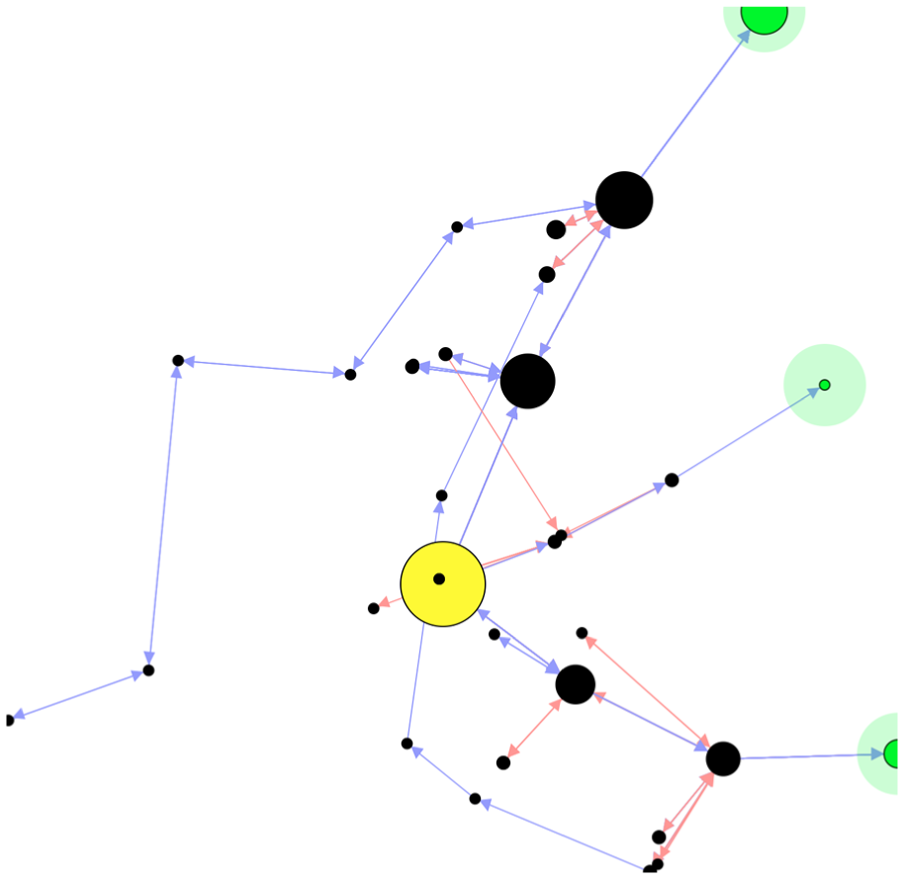
Playtracer applied to the same data as Figure 1. Each circle is a cluster of states, with larger circles indicating more play trace visits to states in that cluster.

Glyph¹⁰ is a recent Playtracer-like state sequence visualization. Like Playtracer, seen states are linked to their observed successors and laid out on a 2D projection, though unlike Playtracer the layout is derived by grouping together states which often transition into each other (rather than from a state-distance metric). The biggest contribution of Glyph is a side-by-side juxtaposition of the state graph just described with a state sequence visualization where each node is a play trace; Glyph collapses state sequences into single nodes, and then lays out those nodes based on their respective distances determined by dynamic time warping (DTW).

DTW is an edit-distance metric like the CCED used by Gamalyzer. Both compare sequences by comparing their individual elements and finding useful alignments between subsequences that are roughly similar. Glyph works with game state sequences (as opposed to Gamalyzer’s action sequences), which requires analysts to define a state similarity function, as in Playtracer.

Another key difference between Gamalyzer and Glyph is generality. Glyph’s metric can be seen as a special case of Gamalyzer where the matching constraints (the warp window, explained in CCED) are relaxed, each action is an emission of the complete game state, and the action-versus-action distance function is the designer-provided state-distance function.

All visualizations that depend on designers defining state difference functions face a key problem: these metrics are not forthcoming for games in general, and generic definitions are impossible. Moreover, gathering up all of a game’s states over time can become expensive if state information is highly detailed. Focusing on actions instead of states sidesteps these problems. Glyph is right to make play traces the object of analysis, and its juxtaposed interface is a substantial improvement over previous work, but we believe action sequences are easier to interpret than Glyph’s opaque, collapsed state sequences.

Audiovisual similarity analysis is a highly generic approach that has been applied to everything from film and music to video games.¹¹ Games with soundtracks or with a significant amount of state encoded in the on-screen display are good candidates for visualization based on chromatic or spectrum analysis. The visualizations commonly used here support a kind of manual edit path or sequence alignment calculation on the part of the analyst, but automating this by devising a metric would be straightforward. The success of this type of visualization suggests that showing alignments or incremental distance measures between two traces might be a useful future direction for visual play trace analytics. As a general approach, interpreting play traces as sentences of actions has proved useful: given a suitable encoding, high-level player strategies have been identified as relations between abstract words¹² that combine abstract actions and some state information. Loh and Sheng¹³ also found that string distance over action sequences adequately captures different player strategy profiles.

Separately from sequence alignment approaches, provenance has been used to describe and visualize dependencies between game states and the actions which produce them.¹⁴ This requires a game-specific mapping from the domain of game objects onto the domain of intentional agents, inert entities, and activities that effect change. This kind of mapping is potentially more involved than Playtracer’s required state-distance metric or Gamalyzer’s input encoding or input-distance metric. Like Gamalyzer, PROV explicitly represents actions, and like Playtracer it emphasizes the available transitions between pairs of states. Unlike both of these, their visualization seems to be tailored for investigating an individual play session, whereas Playtracer and Gamalyzer are both meant for comparing play sessions against each other.

Wender et al.¹⁵ describe a fascinating tool for visualizing Starcraft replays that cross-indexes a log of game events with aggregate information on game states over time. While it is Starcraft specific, the approach does seem generalizable; however, like PROV, it does focus on one trace at a time. We see their trace-based system as evidence that approaches hybridizing state- and action-centric approaches may be superior to either approach on its own; of course, this relies on a robust set of action-centric visualization approaches.

Games with complex generated dialogue or story structures are a natural target for combinatorial visualization. Sali’s work on visualizing visited story nodes in Façade¹⁶ and Prom Week¹⁷ was intended to help system designers understand whether and how their authored content was presented to players, and leveraged both state- and action-centric approaches. Our earliest prototypes were designed to scale this sort of analysis up to larger sets of play traces without losing precision; specifically, we wanted a more robust notion of uniqueness than prefix sharing or event counting, for which we had to develop a suitable metric.

Our play trace visualization was also inspired by visualization projects from the medical informatics community. Medical analysts must find similarities between two patients’ histories, compare treatment schedules, and look for patterns in medical observations without knowing in advance what those patterns might be. The LifeFlow¹⁸ project emphasizes the discovery of anomalous sequences by combining event series into a prefix-tree representation, accounting for misalignment by letting users forcibly align the diagram by a particular shared event. LifeFlow also involves users in merging similar events together, sorting events, and filtering out uninteresting events or sequences. While this interface supports trace analysis, it scales poorly with the number of distinct event types and requires significant analyst interaction. It effectively replaces the human-defined state-distance metrics of Playtracer with a manually enacted trace distance metric. In contrast, our approach sidesteps both the difficulty of defining a game-specific state-distance metric and the lack of scalability of manual trace alignment through the development of a general and effectively computable trace distance metric.

The Gamalyzer visualization

Before presenting the Gamalyzer metric in detail, we will describe our visualization and the requirements it places on the metric. Recall that our visualization should be game-independent, it should group related play traces together, and it should scale to real-world datasets in terms of both performance and visual complexity. It should address game actions rather than game states. And most importantly, we want to visualize whole traces and obtain an understanding of strategies, as opposed to just frequently visited states or common subsequences of actions.

We must immediately discard spatiotemporal visualizations. For one thing, assuming that the game takes place in a simulated space is not justifiable in general (card and dice games often assign no semantics to space beyond here or there). Even when games simulate space, not all game actions are situated in that space. Moreover, in (for example) block-pushing puzzle games, the nature of the physical space changes substantially over time: just superposing states or actions can be misleading. Finally, and worst of all from our perspective, mapping events onto space prioritizes spatial over temporal information, making it tough to compare the relative lengths of traces or the times at which different events occur. Certainly, purpose-built individual visualizations can resolve some of these issues—Tremblay¹⁹ describes a powerful algorithm and visualization for games in which players sneak around a level with moving guards—but here, we are looking for a generic visualization approach. Even Tremblay’s work must assume that enemies follow deterministic paths that do not respond to player behavior, perhaps in part because of the visualization challenges inherent in showing the space of possible scenarios.

Given the importance of wide and frequent branching outcomes to the experience of playing games and the time sensitivity of interactions leading to such outcomes, Gamalyzer supports the discovery of distinct approaches or strategies employed by players. A designer or analyst can view multiple strategies and compare them to each other, or dig deeper into various refinements of a particular strategy. This visualization was originally intended to debug AI general game players by examining their strategies, but the same information is useful for designers targeting human play.

Figure 3 shows a typical Gamalyzer display for human play trace data from the Mario AI Benchmark.^20,22,23 The most prominent features are the colored circles, one for each decision made by a player, in this case actions corresponding to controller inputs. Each polyline connecting those inputs represents a play trace, and time proceeds from the bottom of the image towards the top. As time progresses, it is easy to see how the traces diverge—some earlier than others—and sometimes converge. Traces also naturally cluster together visually. The rounded box shows the currently selected inputs (time points 27 and 28 of the Emil and Keith traces).

Figure 3.

Gamalyzer applied to downsampled human play traces^20,21 from the Mario AI Benchmark²² in the incremental similarity layout (s = 0.005). The mouse is hovering over a pair of traces that is laid out in parallel to each other, with a tooltip showing the actions at the selected time point.

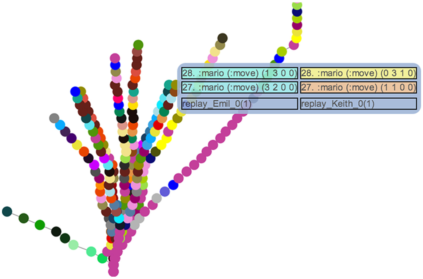
The Mario AI Benchmark receives 24 inputs per second and games last up to 1 min; this has been downsampled to one aggregate action per second to simplify the display. Because it is not possible in general to resample input sequences automatically, the easiest solution here is one that game developers may already be using to minimize the storage requirements of their game metrics: aggregation. This can be implemented when gathering metrics, in a post-processing step on the raw data, or in a custom reader for Gamalyzer (which easily supports new input formats).

For the Mario AI Benchmark, aggregate actions are all of the same type and have four parameters: the number of frames (in this second) spent holding the fireball/run button; the number of frames spent moving rightwards (which may be negative if the player moves left); the number of frames spent holding the jump button; and the number of frames spent holding the duck button. First-person shooter inputs could be aggregated in a similar fashion, for example, by taking the player’s average velocity and number of shots fired during that second. These aggregates do not have to be sufficient for reconstructing the whole play trace, but they serve as a way to smooth over small differences in event order and to reduce the calculation time required by Gamalyzer as well as the visual complexity of the display. Aggregation could also theoretically improve the semantic value of the metric if it captured certain features or context that would be hard to recover from individual traces; but this is necessarily a game- or genre-specific operation. It would be better to avoid using aggregation for that purpose and find ways to parameterize the metric to account for those kinds of concerns.

This downsampling operation is not strictly necessary for the short games being played in the Mario AI Benchmark, but could be important to consider for longer games. A dense representation of play traces—one input per time point—may have visual and computational scaling issues (even in terms of storage) as game lengths increase beyond a few minutes. Gamalyzer’s performance scales linearly with play trace length, but 70 h of play at thirty frames per second still seems out of reach without downsampling, random sampling, or other tricks to drop a few orders of magnitude; compression-based approaches¹² are also worth exploring here. Any visualization that emphasizes sequences will have to contend with this issue, whereas visualizations that aggregate by design can use set representations like Bloom filters that purposely blur time away.

Similar traces are nearer to each other than they are to dissimilar traces, and as traces become more and less similar over time, they converge and diverge. The degree to which incremental similarities influence the layout can be controlled by the user. Figure 4 shows the case where only overall similarity is used. Note that the short trace and long traces are still visually far outliers.

Figure 4.

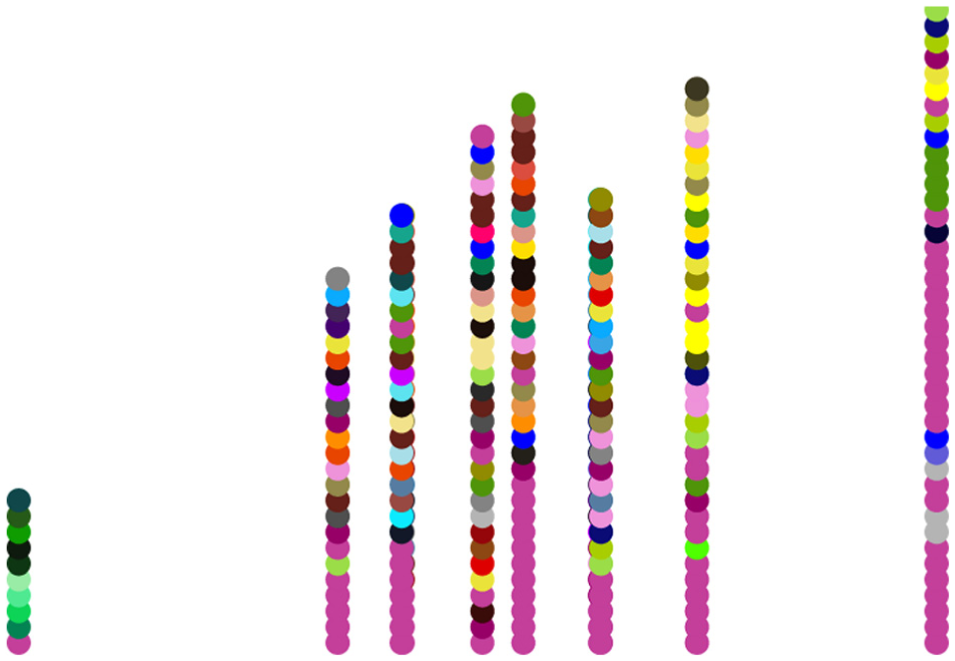
The overall similarity layout (s = 0.000) of the same traces shown in Figure 3. This view more clearly separates traces which may start in similar ways but are overall very different.

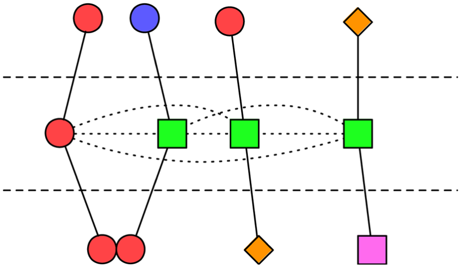
When the user mouses over one or more inputs (inputs may be overlapping), their contents are shown in a hovering information box. Each input is assigned to a particular player and time point (we assume that all traces share the same input frequency) and carries data comprised of a determinant (a category of input, for example, in Chess, a regular move versus castling or a choice of promotion) and a sequence of values (the parameters for that input, for example, where to move, which type of piece to become). Actions with different determinants are not comparable, and actions with the same determinant are similar to the extent that their values are similar. To facilitate visual comparison, different determinants are assigned different glyphs (see Figure 1) and different value combinations are assigned different colors.

Gamalyzer works entirely in terms of actions, not states. We assume that while states are difficult to compare directly, sequences of actions are easier to compare. Even identical game states can carry substantially different design consequences: a player who visits a state once is very different from a player who visits that same state 10 times. We further assume that most players actively pursue goals, so that each trace captures an attempt to achieve one of a small set of objectives relative to the number of traces. The goal of the Gamalyzer visualization is therefore to collate and present players’ strategies for achieving goals so that designers can understand how their game is played in the wild.

To group similar traces, Gamalyzer first uses CCED as a dissimilarity metric, calculating a pairwise matrix of dissimilarity values between 0 and 1. This matrix also has a time dimension, giving pairwise dissimilarity up to a given time point. Gamalyzer uses the overall similarity values—the final time slice of the dissimilarity matrix—to position the final inputs of each trace along the visualization’s X axis so that each pair of traces is as close as possible to its desired distance. This is done using an approximation to classical multidimensional scaling called stress majorization, as implemented by Multidimensional Scaling for Java.²⁴

In general, this is a lossy transformation. Consider three play traces among which each pair has a relative overall distance of 0.5; one example would be the set ${(a, b) (a, c) (a, d)}$ where each trace has two events. There is no way to layout these points along one dimension without violating at least one of the distance constraints, but in two dimensions, this layout is trivial. Different dissimilarity matrices $m_{t}$ require different number of dimensions $d (m_{t})$ for loss-free layout, but the Gamalyzer visualization presents $T$ such matrices, one for each time point. Therefore, we assume without loss of generality that each layer (time slice) is laid out in one dimension; but there is no reason that Gamalyzer could not use two or more dimensions for each layer, given camera controls to facilitate exploration by an analyst.

After the final inputs are placed, Gamalyzer incrementally lays out the earlier inputs to illustrate how play traces converge and diverge over time. Independently laying out each layer using stress majorization or classical multidimensional scaling would be problematic, because these techniques are not stable with respect to the small changes in the distance matrix that accumulate over time. The resulting layouts would be incoherent—a single trace might have inputs spread out and oscillating across the entire width of the visualization. We therefore developed an incremental layout technique that would keep a trace’s inputs relatively close to each other in the horizontal dimension.

Of course, collapsing a high-dimensional metric space onto a single dimension will necessarily be lossy, and the resulting axis positions are not necessarily meaningful on their own. Consider three points in some arbitrary dimensional space which are all equidistant from each other. We could safely project this specific case onto two dimensions, but projecting to a single dimension will necessarily make two of the edges seem shorter than they ought to be, and the points’ position along that single dimension will be totally arbitrary. Their relative positions, especially with respect to other points far away from these equidistant points, can be interpreted—if there are many points which are far away from these three, the three points might even completely overlap in the projection. Gamalyzer visualizations therefore do not include any horizontal axis, since absolute horizontal position is meaningless and the visualization is meant to be interpreted loosely; applications that need precise distance information should work in metric space rather than in the visualization’s low-dimensional projection.

Earlier slices of the dissimilarity matrix provide soft geometric distance constraints between the corresponding inputs of each pair of play traces at each time point. These are expressed as link distances in the force-directed layout component of the Data-Driven Documents visualization framework (d3.js).²⁵ The user can control the strength, s, of these soft constraints—how tightly traces are pushed apart or drawn together based on (dis)similarity—to explore the relationships between play traces and their similar subsequences. Figure 5 illustrates the constraints at work at a single layer of the incremental layout. Note that while the lowest level of inputs is drawn, Gamalyzer has not in fact laid them out in any way; the upper layer strongly determines the X coordinate of the middle layer’s nodes, while the dotted-line constraints among middle-layer nodes weakly shifts the polylines left or right according to s.

Figure 5.

Constraints used during incremental layout (center row).

As s increases, instantaneous differences dominate gestalt differences and it becomes difficult to follow an individual trace through time. If s is too low, shared motifs become more difficult to spot. Intermediate strength values give good separation to slightly different trace segments while still drawing together somewhat-similar trace segments (see Figure 6). Reasonable values for s range between 0.000 and 0.005; at higher values, layouts become too chaotic to read and there are no new insights. In general, we view 0.000, 0.002, and 0.005 as key interesting values for s. s = 0.005 could be seen as the default setting, since it shows overall differences and how groups of traces diverge over time. s = 0.002 can be used if s = 0.005 is unclear, perhaps because many traces are quite similar (but not identical) on the moment-to-moment scale. s = 0.000 strongly shows the overall differences and is useful especially if many traces share a common prefix or have shared motifs that are not important to the analyst.

Figure 6.

Intermediate link strengths (s = 0.002) separate slightly different traces (see the highlighted inputs) while still drawing together somewhat-similar trace segments (compare Figures 3 and 4).

Interactivity

Users can select traces or inputs to reveal extra information by dragging out selections over the Gamalyzer visualization or by using a hypothetical auxiliary state visualization (to answer, for example, “How did the character get to this position?” if the state visualization is a heatmap, or “How did this quantity exceed this amount?” if the state visualization is a plot of values over time).

We investigated the Refraction dataset (the same featured in Playtracer’s presentation⁸) for a qualitative comparison of Gamalyzer and Playtracer along these lines. The tasks were to identify distinct solutions for a given Refraction puzzle and to appraise players’ skill levels. Gamalyzer revealed aspects of play traces (e.g. durations, orderings, and cycle characteristics) that Playtracer was not capable of showing, although as expected the state-centric tool did a better job of showing when different players reached identical states.

These are important properties for designers to know about: Playtracer can show a tangent that was abandoned, but Gamalyzer can show how many moves that diversion took; Playtracer can show that two players tried three approaches before reaching a solution, but Gamalyzer can tell a designer if both were always tried in the same order; Playtracer can show that a player visited a handful of states and then gave up, but Gamalyzer can show that player repeatedly trying and failing at the same approach.

We saw the best results when Gamalyzer and Playtracer were used in concert: identifying interesting trace clusters in Gamalyzer and interrogating them in Playtracer, or vice versa. This suggests that while the Gamalyzer visualization can be used by itself to enumerate strategies, readability is improved by an auxiliary, state-centric visualization. The goal of this juxtaposition is to give a quick impression of the state reached by a sequence of actions. One generic approach to this state visualization might be to automatically run the game up to a selected time point, giving inputs based on the trace or traces selected by the user, and to show the resulting states as superposed screenshots in the Gamalyzer interface. Even a simple technique like this would satisfy much of the need for concrete state visualization alongside Gamalyzer, given a complete encoding and deterministic replay.

Trace-selection

The visualization described above works well for small number of traces. It is clear that it would become quite noisy with hundreds or thousands of traces. Moreover, the layout constraints used are somewhat expensive to compute (more so, in fact, than the distance metric itself, whose results can moreover be easily cached). To resolve these issues, we wanted to highlight and, if possible, limit our processing to only the most interesting play traces.

While almost every play of a game is unique, most are different in trivial ways. In Figure 3, for example, only one of the third and fourth traces from the left is necessary to understand the strategy space. Since their overall difference according to the Gamalyzer metric begins and remains small, they are redundant in a measurable way. It suffices to show just one of them as an exemplar, standing in for the other. If we pick the right traces to capture the interesting strategies as representative examples and summarize the remainder of the population, we can gain both visual simplicity and efficiency without sacrificing too much precision. We can also provide special interactions to zoom in on particular bundles of mostly similar traces for more detailed exploration.

Automated graph layout is by nature an expensive operation, so the graph-layout community has had to solve essentially the same problem. Brandes and Pich²⁶ developed a linear-time approximation to multidimensional scaling by selecting relatively few nodes (variously called “pivots” or “landmarks”) and laying out the graph relative to those pivots instead of the full population of nodes. This works because usually a small number of nodes determine the overall shape of the graph.

Brandes and Pich evaluate two methods of pivot selection: random choice and the maxmin strategy, which picks the first pivot arbitrarily and selects each subsequent pivot to be the datum which has the greatest (max) least (min) distance from all currently selected pivots. In other words, maxmin always chooses a node which is most unlike any of the previous pivots. While Brandes and Pich are selecting a subset of nodes in their work, we are finding a subset of traces which themselves comprised multiple actions and laid out as multiple nodes in the final visualization. We adapt their approach by treating complete traces as points in a high-dimensional metric space, selecting pivots among those high-dimensional points using the maxmin strategy, and finally performing a separate visual layout of the inputs of the traces which pivot selection determined were the most important. Brandes and Pich also prefer the maxmin strategy, because it reaches good layouts with a much smaller number of pivots than the random strategy: it captures more significant samples more quickly.

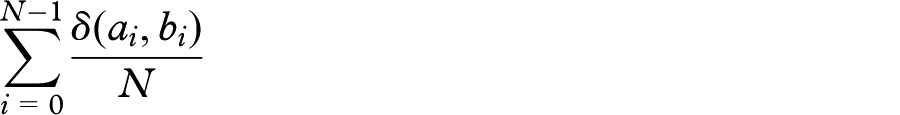
We select as pivots the most interestingly distinct play traces, and count for each pivot what proportion of traces are more like it than they are like any other pivot. This counting comes at no additional computational cost, since we have replaced the $N^{2}$ distance comparisons with $k \times N$ comparisons (where $k$ is the number of pivots). The number of exemplar traces could be determined automatically (by continuing until the maxmin value reaches a threshold) or given by a parameter; so far, we have found a tunable parameter suffices, allowing the user to work at any precision.

Pivot selection foregrounds the traces that add the most substantial information about the game’s strategic landscape. While we use a fully automatic method here, it stands to reason that users could select certain traces as pivots manually to orient analysis around particular traces, perhaps for comparative analysis.

The Gamalyzer metric

The Gamalyzer visualization aggregates similar traces. But what does similar mean? To answer this question, we turned to the body of knowledge on sequence clustering, a familiar (but open) problem in the speech recognition and bioinformatic communities (among others).

Briefly, the problem of sequence clustering is to take sequences of symbols (e.g. component molecules) and determine whether they belong to one group (e.g. a protein family) or another; or, in the unsupervised case, to determine how many distinct groups there are and how closely a given sequence of symbols matches each such group. Two approaches are generally used: discriminative methods locate shared structure and interpret the degree of sharing as a feature for use with a traditional clustering algorithm;²⁷ and generative methods learn statistical models (often hidden Markov models) from data, measuring similarity as the likelihood that a given statistical model would generate a candidate sequence.²¹

Gamalyzer uses a discriminative technique, applying CCED³ to sequences of game inputs. For our purposes, discriminative methods are easier to explain and encode fewer assumptions about the underlying game and player models than generative methods do. Our method is also reasonably efficient, scaling only linearly in the lengths of the sequences (thanks to the constraints) and in the number of sequences (as described in trace-selection).

Edit distance is a measure of how dissimilar two sequences are based on how many edit operations—insertions, deletions, and matches—would be required to change the first sequence into the second. We borrow three chief insights from CCED and related techniques: first, we can consider changes instead of matches; second, not all changes are equal (e.g. changing a 9 to an 8 may be easier than changing it to a 6, and changing it to a 1 may be impossible); and third, we can constrain the allowed edit operations to improve efficiency and avoid degenerate cases such as deleting the entire first sequence and inserting the entire second sequence.

Gamalyzer assumes that all measured sequences share a common clock rate, but it may be possible to automatically insert “no-op” events to synchronize two sequences; at any rate, we leave that for future work. Taking insertion and deletion costs to be equal (and both 1), we calculate the cost of changing one specific input into another using an input (as opposed to input sequence or state) dissimilarity metric. If such a change is not possible, then the input must be deleted or an input from the other sequence must be inserted. Given these costs, CCED finds a globally optimal edit path.

Inputs comprised two primary terms: a type (or determinant) and a value. If two inputs have distinct types, they are incomparably different kinds of decisions; changing one to the other is not possible. To compare the values of two inputs with the same type, we must rigorously define what those values are and how to determine their similarity.

For example, numeric values might be normalized to their possible domain and the distance could be their absolute difference (or some non-uniform distribution could be assumed). The difference between string values might be 0 if they are identical and 1 if they are distinct; or we might take string edit distance as the difference. Events could also have compound values such as lists of parameters, and these might be compared via weighted difference. These data types and comparators are opaque to Gamalyzer, which is always parameterized with a specific input-wise dissimilarity metric $δ (a, b)$ . Our implementation provides (and the text so far assumes) a relatively generic $δ$ function and data schema which assumes that each input’s value is either an ordered list or unordered set of numbers, non-numeric tokens, or nested lists and sets; the details here are reproduced from the original Gamalyzer paper.¹

Numbers are normalized according to their observed domain (in the whole set of traces) and their normalized distance gives a dissimilarity value. We assume here a uniform distribution, but other distributions (e.g. Bernoulli, Gaussian) are possible.

Non-numeric tokens are completely distinct ( $δ (a, b) = 1.0$ ). There is room here to add sophistication by considering probabilistic distributions of atoms.

The difference between two unordered sets $a$ and $b$ of length $N$ is the sum

\sum_{i = 0}^{N - 1} \frac{δ (a_{i}, b_{i})}{N}

The difference between two ordered lists $a$ and $b$ of length $N$ is the sum

\sum_{i = 0}^{N - 1} \frac{(N - i) δ (a_{i}, b_{i})}{\sum_{j = 1}^{N} j}

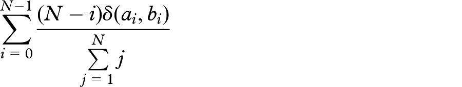
Each successive term in the list is discounted linearly and normalized so that the maximum value of the sum is 1.

Since Gamalyzer is game-agnostic, designers must have some way to inform the metric about game-specific notions of similarity. This is exclusively done by defining the input types, the possible values taken by inputs, and the $δ$ functions used to compare the values of inputs with identical types. Taken together, we call these a game’s encoding for Gamalyzer (so far, all games we have considered have used the default $δ$ function). These encodings will be game-specific, but it should be straightforward to use a game’s existing telemetry to produce the input types and their value schema. Furthermore, defining an input-versus-input dissimilarity measure should be much easier than defining a play trace-versus-play trace dissimilarity measure. In our experience, such a measure naturally follows from the input types’ possible values, as did our default $δ$ function. Of course, the designer may supply any arbitrary $δ$ function and syntactic encoding—the default function above is just a generally useful approach. A further discussion of encodings is given in Gamalyzer Encodings.

Given such an input-against-input dissimilarity function $δ$ , the continuous edit distance (without constraints) for changing the input sequence (play trace) $A$ into the input sequence $B$ can be defined by the recurrence³

Δ (A, B) = \min {\begin{matrix} Δ (A, B_{Rest}) + \cos t_{ins} (B_{First}) \\ Δ (A_{Rest}, B) + \cos t_{del} (A_{First}) \\ Δ (A_{Rest}, B_{Rest}) + δ (A_{First}, B_{First}) \end{matrix}

If $A$ (respectively $B$ ) is empty, we insert (respectively delete) inputs until both sequences are exhausted. In this way, every pair of inputs ( $A_{i}, B_{j}$ ) from both traces is compared to find the minimum value of $Δ (A, B)$ . This value is then normalized by the sum of the lengths of the two sequences (multiplied by the deletion and insertion costs, respectively) to give a value between 0 and 1: the Gamalyzer metric. Being a dissimilarity metric, this is larger for less similar traces and smaller for more similar ones.

Since many of the intermediate minima found during this recurrence will be reused, it is traditional to use a dynamic programming implementation. We fill out an $| A | \times | B |$ array starting from the initial pair so that the value at index $(i, j)$ is the edit distance $Δ (A_{0 . . i}, B_{0 . . j})$ for the corresponding subsequences of $A$ and $B$ . We then find the optimal path by tracing backwards from $Δ (A_{0 . . | A |}, B_{0 . . | B |})$ towards the origin. We chose this bottom-up approach because it afforded easier implementation of global constraints on the search as described in the next section: these constraints amount to avoiding certain regions of that array. A useful consequence of this algorithm is that we obtain not just the cost of changing one play trace to another but also the entire sequence of edit operations and the partial costs up to each step in that sequence. This means that we could show users of Gamalyzer not just how similar entire play traces are, but also how these traces become incrementally more or less similar over time.

CCED

CCED is so called because it adds two constraints to continuous edit distance:³ the Sakoe–Chiba Band²⁸ and the Itakura²⁹ Parallelogram. These are both envelopes (or warp windows) that constrain the permissible area of the $| A | \times | B |$ edit matrix. Intuitively, both prevent degenerate matches of early parts of one sequence against late parts of the other sequence. The Sakoe–Chiba Band ensures that no time points which are further apart than the window can be matched against each other, and the Itakura Parallelogram gives a window which is small at the beginning and end of the sequences but larger in the middle. In other words, the former constraint prevents traces which are too different overall from being comparable (i.e. having a dissimilarity less than one), and the latter constraint requires that comparable traces begin and end in similar ways. In a speech recognition context, the Sakoe–Chiba Band ensures that the “th” in “thick” is not a good match for the one in “bath,” and the Itakura Parallelogram makes the pronunciation of “crawfish” comparable to “crayfish” but not to “dolphin.”

Both constraints make sense for speech recognition, but gameplay traces invalidate the assumptions of the Itakura Parallelogram: even given similar goals and strategies, not every trace will begin or end with similar actions. Under the Itakura Parallelogram, two traces which are similar up to a certain point but then diverge (or traces which begin differently but then converge) would be punished heavily. We would be forced to ignore their common prefix (resp. suffix) because their suffix (resp. prefix) was too different. We therefore use only the Sakoe–Chiba Band to constrain matches. Adopting constraint with envelope width $ω$ means that the performance of the dynamic programming approach can be improved from $O (| A | | B |)$ to $O (| A | ω)$ —linear in the length of the first sequence. We assume that $ω$ is provided by the designer, but it is straightforward to imagine reasonable defaults based on median play trace lengths.

Gamalyzer penalizes differences in play trace length using global constraints, insertion costs, and deletion costs. When the window is narrow relative to differences in length between sequences, sometimes no edit path can be found; in this case, it is not only fair but also desirable to assume complete dissimilarity. We believe this is justified if the time ordering of moves is important; if earlier moves substantially influence the game state, similar moves that occur later on are taken in a different context and their seeming similarity is therefore only superficial.

Consider a player jumping over an obstacle: we would not want one player’s hop over the level’s first obstacle to match against another player hopping over its last obstacle. Those are similar actions, and if we were doing N-gram analysis or motif detection, we might be interested in that similarity, but in terms of analyzing the entire play trace, this is a nonsensical matching.

Our unoptimized, single-threaded implementation in the Clojure Lisp dialect (which targets the Java virtual machine) takes 5 s to compute a $100^{2}$ dissimilarity matrix for synthetic traces averaging 44 inputs long on a 2.6-GHz Intel Core i7 laptop (using negligible RAM). In practice, the metric would not be calculated $N^{2}$ times, but $k \times N$ times, where $k$ is the number of pivots (see trace-selection) and $N$ is the number of traces. This gives a scaling behavior which is linear instead of quadratic in the number of traces (and also linear in the length of traces). In terms of asymptotic complexity, this is about as good as could be hoped for in the absence of extensive indexing or pre-processing.

That said, constant factors remain an issue. Considering all 40 levels of the Mario dataset at full precision, we have 400 play traces averaging around 800 inputs in length (with some traces as long as 1400 inputs). Finding each additional pivot point in this moderately sized set takes around 18 s, and laying out the diagram takes roughly 20 s (most of which time is spent building visual elements for display). We believe these constant factors could be substantially reduced by moving to a language designed for computational efficiency (a preliminary, unoptimized re-implementation in Rust won two orders of magnitude improvement); by executing several trace-versus-trace distance calculations in parallel during pivot selection (a probable linear speedup with the number of processors); and by taking advantage of CPU cache with more compact storage or more sophisticated algorithms.³⁰ In fact, all of these distance calculations could be done incrementally or offline, since traces are assumed to be immutable, performance of the metric currently poses no theoretical barriers to interactive use.

The diagrams in this article were each produced in well under a half a second; this time includes both the calculation of the required distances and browser layout and rendering via d3.js. Our diagrammatic layout could be made even less expensive by approximating our layout constraints more coarsely or by using a different and less memory-intensive renderer than a web browser.

Gamalyzer encodings

As earlier evaluations of Gamalyzer showed, the metric is sensitive to the choice of action sequence encoding. The two main questions to consider are when actions are emitted and what the actions are like. In the Super Mario example, we came to understand that one action per frame was less useful than one action per second.

After deciding on the rate at which events are generated, the designer must consider what types of input there are, and how are they parameterized. In other words, what are the axes of difference which are relevant to the questions that the designers have about their game? We illustrate these concerns with examples.

In Chess, we want to pick input types and values that will foreground distinctions in strategy. As a first attempt, we might say that there are regular moves and castling moves, where regular moves are parameterized by a player, a piece, and a destination, and castling moves are parameterized by a player and a direction. Pieces are uniquely identified (player 1’s king’s bishop, player 2’s third pawn, etc.) and destinations are coordinate pairs. Castling moves have a difference of 1.0 if the players are different, 0.5 if the players are the same but the directions are different, and 0.0 if both are identical. Regular moves have a difference of 1.0 if the players are different; otherwise, add the piece difference and the position difference, where the piece difference is 0.0 if the pieces are identical, 0.3 if the pieces have the same type, and 0.6 otherwise, and the position difference is the [0, 0.4]—normalized Manhattan distance between the two positions. This reflects the insight that the type of piece matters more than the destination position when considering Chess moves.

While this suffices to describe all plays of Chess, it is poorly suited for Gamalyzer because it is highly context-sensitive and puts too much of the burden of difference into values rather than types. Captures are more significant than regular moves from a designer’s standpoint, en passant captures are even more surprising, and piece promotions are important enough that they should show up in the metrics. We can obtain more useful results if we break up the original encoding’s regular moves into moves without capture, moves that cause capture, and en passant captures; all three can use the same input value schema (player, piece, and destination) and $δ$ function. It may even be worth separating castling into separate castling-left and castling-right input types. Finally, we add a piece promotion event with the values being the player, the pawn involved, the promoted rank, and the position at which the promotion occurred; if the players are the same, two promotion events can be compared as a weighted sum of which pawn was involved, which rank was chosen, and the Manhattan distance between the promoted positions. With this encoding, more of the flavor of each match is surfaced in the Gamalyzer output difference.

For a real-time game like Super Mario Bros., we are interested in frame-by-frame inputs. If we were to create one Gamalyzer input event for each button (jump, move right, move left, or run), then some frames would yield several inputs and some frames would yield no inputs; this would make it hard to represent simultaneous actions and, more importantly, it violates Gamalyzer’s assumption of a common clock rate among input sequences. Since simultaneous actions are possible, we must represent player input as the set of buttons held on a given frame; we will give all such inputs the determinant move. Among the buttons, running is the most significant predictor of style,³¹ so we use a weighted ordered list of numbers $(Bt n_{Run}, XDirection, Bt n_{Jump}, Bt n_{Duck})$ , prioritizing the four types of input in that order. Each value represents whether the corresponding button was held (0 or 1) or the direction in which the player wanted to move (−1, 0, or 1).

We used our prior knowledge of Mario play to devise a good Mario input encoding. When we applied Gamalyzer to the social puzzle game Prom Week,³² we worked with that game’s designers to devise two reasonable encodings.

Prom Week

Prom Week serves as an interesting use case for Gamalayzer, as it is a game that defies typical genre descriptions. The designers of Prom Week have referred to Comme il Faut,³³ the AI system that underlies the game, as a “social physics” engine since it allows for myriad social forces to dynamically determine the behavior of the game’s characters. Consequently, the game itself has been called a “social physics puzzle game.”

Players are given social goals to complete, such as having two estranged friends make peace, or helping a social pariah claw their way to the top of the high school hierarchy. To complete these goals, the player selects pairs of characters to engage in social exchanges; these are activities such as bickering, reminiscing, and asking each other out on dates. The set of available social exchanges is determined through an evaluation of the game’s social state and represent the desired actions of the game’s characters. Moreover, each selected social exchange alters this social state, affecting the exchanges available in subsequent turns.

To successfully complete the game’s goals, players must massage the social state so that the desires of the characters are in line with the desires of the player. Each campaign of the game can be solved in many ways, and as such a mechanism such as Gamalyzer to discern common and uncommon strategies of play would be of great utility to the game’s designers. Since its initial release on 14 February 2012, over 100,000 play trace files have been generated, making Prom Week a good candidate for developing novel forms of visualization.³⁴

Each move in Prom Week has the player select an initiating character, a social exchange, and a target character. In the first encoding ( $gl z_{ie > t}$ ), every input has the same determinant (move); the social exchange’s initiating character (i) has the same relevance as the combination of social exchange (e) and social intent (a social exchange category); and both of those have greater relevance than the target character (t). The second encoding ( $gl z_{intent}$ ) puts the intent into the determinant and treats the initiator, social exchange, and target as equally important.

These encodings carry different design knowledge. In the former, it is assumed that every input is roughly comparable; in the latter, pursuing different social goals—improving friendship, beginning to date, becoming enemies—is treated as making fundamentally different maneuvers. If using one encoding rather than the other makes Gamalyzer agree better with Prom Week designers’ perception of dissimilarity, that tells us something about Prom Week: either social intent is one component of strategy among many, or else it is the primary indicator of player intention.

For a concrete example of each encoding, consider a turn in which the player wants Chloe to flirt with Doug. Here, the initiator is Chloe, the target character is Doug, the social intent is to increase Doug’s romantic affection for Chloe, and the specific social exchange is flirting. In the $gl z_{ie > t}$ encoding, the input’s determinant is move and the value contains Chloe, Flirt, and Doug, with Doug in a less-important position; in the $gl z_{intent}$ encoding, the determinant is romanceUp and the value contains Chloe, Flirt, and Doug in equal prominence.

We found that using a greater number of distinct determinants produced better (more designer-comprehensible) results. This carried through to unpublished work applying Gamalyzer to puzzle games: in general, we feel that if traces are short, then it helps to use more distinct types of determinant, whereas longer traces benefit from the increased blurring that shared determinants provide.

Using Gamalyzer

Gamalyzer is a general-purpose approach and its core metric and layout algorithm are relatively simple (assuming access to a force-directed layout, multidimensional scaling, or constraint satisfaction library). A prospective user can apply Gamalyzer to their own project either by using our existing implementation or by reproducing the central algorithms in their own codebase or analytics pipeline. The only precondition is that the game must be instrumented to capture enough moment-to-moment information about player activity to reconstruct action sequences for analysis. This may already be the case for games with persistent Internet connections; otherwise, modifying source code to record game actions, storing these action sequences, and transmitting that information to centralized data stores is outside the scope of this article (we refer readers to the game analytics literature for the particulars⁷). Recall that Gamalyzer works on play traces, which are sequences of actions tied to a particular play session or player. Any technique that can construct these traces from recorded data (producing a Gamalyzer encoding) will suffice to provide input to the metric and visualization.

The second step towards integration with Gamalyzer is to calculate the metric for pairs of play traces in a given encoding. Our reference implementation is distributed as a Java library. The data structures it uses as input can be built directly by client code, read from a generic data format (Extensible Data Notation³⁵), or read in a game-specific way by defining a reader function. Analysts may instead choose to reimplement the metric on their own, which can be done in a dozen lines of code.

With a function for calculating the distance between two traces, an analyst can now prepare the inputs to the visualization. Our implementation provides a web service that maps different URLs onto requests for data from particular games; the path refines this request to cover particular levels, players, or other sub-divisions mirrored in the directory structure of the trace files on disk. A configuration file in each game directory provides game-specific settings describing the format of the files, which reader function to use, and so on. It would be straightforward to extend this code to perform database queries or access other data sources.

After loading the traces, we build a set of pivots and count how many traces are represented by each pivot (see trace-selection); then, we calculate the overall trace layout using multidimensional scaling and send all of these data to the client for rendering. Any re-implementation could follow similar steps, specialized to the game in question. Our code performs all this on demand, but the calculations could also be cached, re-done as new traces are collected, or revised in a scheduled batch process. Finally, our client-side visualization code makes a request for a particular user-provided URL, determines glyphs and colors to assign to each input, and then builds the graphical display described in The Gamalyzer Visualization.

Gamalyzer was originally designed to sanity-check the behaviors of a general videogame-playing agent. The metric and visualization are agnostic to the source or semantics of player actions: we can analyze not only machine- or human-generated gameplay actions (though that has been the focus of our evaluation and other work) but any representation of semantic game trace properties as structured syntax. These representations of semantic information as syntax can even be augmented by including state data within the actions comprising the trace.

For example, in a stealth game, we may have a prior belief that player movements mean something different when the players are undetected as opposed to when they are under suspicion or fleeing. We could thus encode the player’s movement actions as one of three different types of action depending on status, or include a danger property in the move action. Emitting whole game states at each frame is also worth exploring and evaluating in more detail: is Gamalyzer’s advantage specifically because it analyzes sequences, or is it because it analyzes actions?

We may also pick different encodings depending on our design query. If we wanted to know whether enemies ever exhibit unusual behaviors, we may choose enemy behaviors or enemy states as our action sequence. Other debugging tasks could also be Gamalyzer-assisted: emitting an event when an art asset needs to be loaded from disk, or when a frame takes longer than a sixtieth of a second, along with events describing player actions to correlate player activity and performance issues. In the context of competitive games, we could answer questions about the global population of strategies by looking at sequences of games rather than sequences of actions within an individual game.

Another notable feature of Gamalyzer’s assumptions is that they can be satisfied by activities that are not games at all. Any goal-directed sequence of actions is a candidate for analysis with the Gamalyzer metric (and, indeed, the Gamalyzer visualization). This includes task-oriented computer usage (such as game designer modeling³⁶), medical treatment history, and conversational AI.

In summary, our approach (a lexicographically weighted product order) is lightweight compared to asking designers to define an input-distance function, simple to explain by example, usable without perfect knowledge of Gamalyzer’s inner workings, and easy to integrate into existing game metric instrumentation—either by altering the game’s metrics output or through a post-processing step. Gamalyzer does not require the use of this specific dissimilarity function, but we provide it as a generally useful default; replacing it with a different function is straightforward but might reduce generality.

Evaluating Gamalyzer

The Gamalyzer visualization depends on the Gamalyzer metric surfacing meaningful differences between play traces. We have evaluated the metric in several different contexts of use and game genres;^1,4 the results here are reproduced from these previous publications. We also note that other string-distance-based metrics have been shown to be consistent with designer perception,¹³ and these independent results reinforce our own.

In the paper introducing Gamalyzer, we synthesized play trace data from an artificial game and also checked Gamalyzer’s results against the hand-tuned Super Mario Bros. player clustering reported by Holmgård et al.³¹

Identifying artificial player models

First, we wanted to know if Gamalyzer could identify typical examples of player strategies. Our synthetic data experiment evaluated Gamalyzer against 1000 sets of 60 traces each, where each trace was drawn from one of three models of an abstract game with three similar (but distinct) moves. Each model preferentially selects one among these three inputs, modulated by a noise percentage by which inputs are pulled from a different (randomly selected) model. We increased this noise to understand how Gamalyzer’s discriminative performance degraded as noise increased.

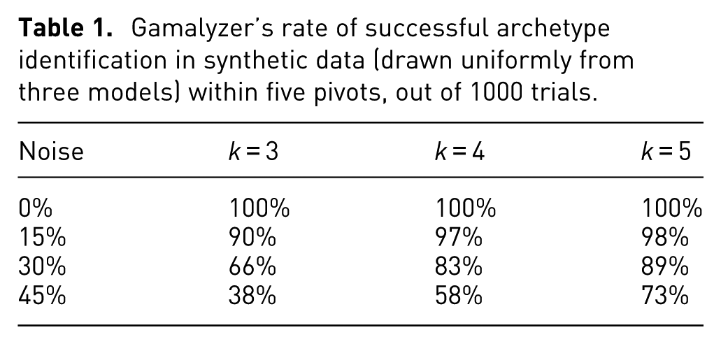
Table 1 shows Gamalyzer’s success rate in picking out the three models (i.e. selecting at least one instance of each of the three models as a pivot) from increasingly noisy data with three, four, and five pivots. Each row uses the same 1000 sets of synthetic traces, but selects an increasing number of pivots. Even when all three models are not recovered, two distinct models always appear among the traces, and the redundantly selected pivots are at the fringes where models act like each other. The synthetic data experiments suggest that Gamalyzer’s distance metric successfully identifies distinct player strategies when applied to a dataset with noisy play traces from a finite set of player models. Moreover, if the goal is only to identify all of the models, the number of pivots can be increased until an error threshold is met.

Table 1.

Gamalyzer’s rate of successful archetype identification in synthetic data (drawn uniformly from three models) within five pivots, out of 1000 trials.

Noise	$k = 3$	$k = 4$	$k = 5$
0%	100%	100%	100%
15%	90%	97%	98%
30%	66%	83%	89%
45%	38%	58%	73%

Mario player clustering

Next, we wanted to investigate the semantic value of the Gamalyzer metric. The play trace similarity measures used by Holmgård et al.³¹ were based on hand-selected features and seemed to be both well motivated and effective at distinguishing how players moved through a level, so we used the clusters found in that work (along with their method of clustering) as a baseline. Gamalyzer is sensitive to the level in which play traces take place, so we planned to compare a clustering based on the Gamalyzer metric for each level against the corresponding tagged player data for each level.

We then compared the quality of each pair of clusterings (the baseline clusters and those found by Gamalyzer for a given level) using Adjusted Mutual Information—specifically, $AM I_{\max}$ . $AM I_{\max}$ is an information-theoretic measure tuned for small number of items relative to the number of clusters which discounts any similarities that could be due to chance.³⁷ Any value above 0 indicates that the two clusterings are more similar than would be expected by chance, and a value of 1 means that the two clusterings are identical.

Our results are summarized in Table 2. Across the 40 levels, we found an $AM I_{\max}$ of 0.28 with a standard deviation of 0.26. The high standard deviation was caused by levels where only one cluster was attested in the baseline data; these (trivially) perfect alignments skewed the distribution. Ignoring those levels, we found a mean of 0.22 with a standard deviation of 0.17. These values indicate that the manual feature selection and the Gamalyzer metric gave clusterings which were substantially more similar than could be expected by chance alone.

Table 2.

Mean $AM I_{\max}$ of different sets of traces across different sets of levels.

$AM I_{\max}$	All levels	Interesting levels
All traces	$μ = 0.28, σ = 0.26$	$μ = 0.22, σ = 0.17$
Similar durations	$μ = 0.44, σ = 0.30$	$μ = 0.32, σ = 0.16$

Any value above 0 indicates that the two clusterings are more similar than would be expected by chance, and a value of 1 means that the two clusterings are identical.

One significant difference between the Holmgård et al. feature vector and the Gamalyzer metric is that the former is duration-insensitive. A play trace which perfectly followed the target path for 5 s before falling into a pit would receive a high similarity score according to the feature vector even though the AI’s behavior is much more diverse when considering the whole level. Gamalyzer would treat this pair of traces as similar at first, but strongly divergent overall (we suspect that large differences in trace length will be of significance to human designers as well). We performed an additional experiment to investigate how much this artifact of the different approaches impacted the clusterings.

For this analysis, we dropped from each level any trace whose duration was more than one standard deviation away from that level’s mean. We removed these traces from the (post-clustering) tagged Holmgård et al. dataset and from the (pre-clustering) input to Gamalyzer. This difference in treatment was justifiable: a feature-based score is independent of which traces are included in the clustering, so removing individual samples’ post-clustering should not have a significant impact on the overall clustering; in Gamalyzer, however, all distances are relative to other traces, and removing those distances amounts to removing the pre-clustering data point. When all traces were of similar length, we saw an $AM I_{\max}$ of 0.44 with a standard deviation of 0.30 when including levels with only one cluster and an $AM I_{\max}$ of 0.32 with a standard deviation of 0.16 without those levels. This reinforced our intuition that much of the difference between the clusterings was due to time sensitivity.

Overall, we found fairly similar clusters to those determined by the hand-selected and hand-tuned feature vectors from Holmgård et al. This was achieved solely by determining an order among the properties of player inputs—namely, considering running as the most important aspect of player intention, followed by moving right and jumping—and clustering based on the Gamalyzer distance metric under that assumption. Humans still have a role in this process, but the play trace features under examination fall naturally out of the game design and do not require substantial effort in defining or calculating time-varying features of the game state.

Prom Week

Our next step was to check the assumption that Gamalyzer faithfully represented designer-relevant differences, as opposed to merely identifying syntactic differences in play traces. For their previous evaluation and visualization work, the Prom Week developers had already recorded every gameplay action made by players. This dataset was therefore an attractive target for Gamalyzer.⁴ The first author wrote a simple program to translate their existing action traces into several distinct Gamalyzer encodings; we then conducted several experiments measuring the Gamalyzer metric’s suitability for various designer-relevant purposes. We must emphasize that this, too, is an evaluation of the Gamalyzer metric, not the visualization.

In designing our experiments, we supposed that one feature that play trace comparison has in common with image comparison³⁸ is that most distances, on a 0–1 scale, are likely to be close to 1: so different as to be effectively incomparable. In our case, we were not trying to derive the features that humans use to discern play trace differences; instead, we were trying to validate that the distances found by various metrics conform to the distances determined by humans. The experiments conducted by Russell and Sinha³⁹ comparing the L1 and L2 distances for image dissimilarity were a closer match for our aims. Here, the authors also controlled for semantic content so that human ratings purely concerned the visual properties (rather than the subjects) of the image. Semantic content is the whole point of play trace analysis, so our experimental design borrowed techniques from both studies.

We compared Gamalyzer against three baseline dissimilarity metrics that had appeared earlier in the literature around Prom Week: 1-grams, the normalized Manhattan distance between counts of social exchange action names;⁴⁰Interactions, the normalized Manhattan distance between counts of interactions (the intent, initiating character, and target character); and States, the angular dissimilarity between the numeric parameters of the game state (as opposed to the earlier baselines, which considered game actions).

These baselines were evaluated along with two Gamalyzer encodings (described in sec:encodings) in three experiments (results are shown in Table 3). The first task asked designers to rate play traces in terms of their relative difference from a reference trace. The metrics were evaluated based on their agreement with this appraisal.

Table 3.

Root-mean-square error results for all metrics in the Prom Week study.

	Dissimilarity	Outliers	Uniqueness
$gl z_{intent}$	0.208	0.279	0.189
Interactions	0.219	0.292	0.173
-grams	0.236	0.304	0.242
$gl z_{ie > t}$	0.287	0.326	0.290
States	0.592	0.557	0.576

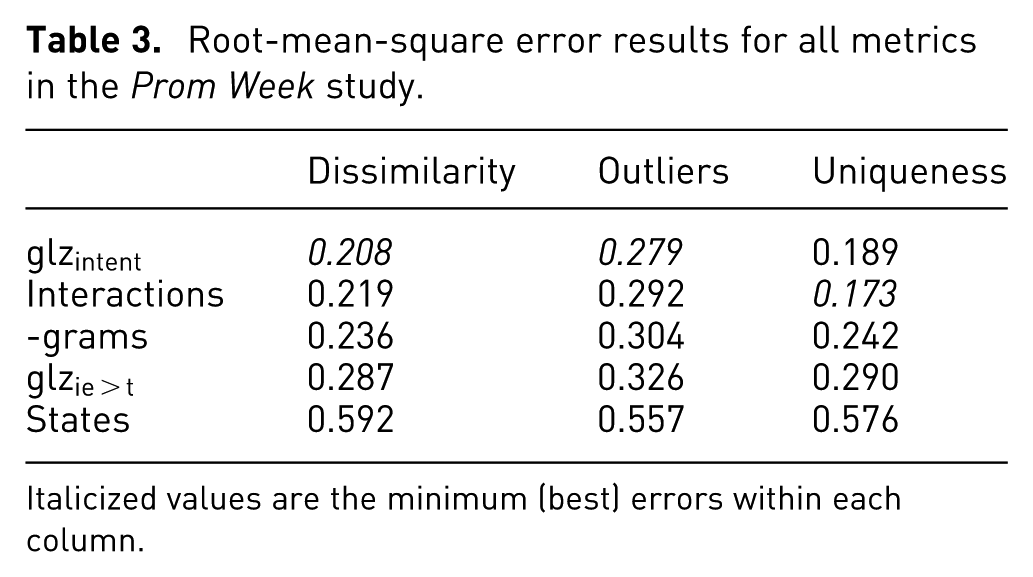
Italicized values are the minimum (best) errors within each column.

We also considered the problem of presenting a sorted list of outliers to a designer; this could highlight players who are misunderstanding a system, or who are playing to sabotage or circumvent it. To determine the degree to which each play trace is an outlier, we formed an operational definition of “outlier-ness” in terms of distances between play traces. Then, we asked designers to identify how well each trace of a set of traces fit into the set as a whole; the best metric was the one for which the outlier statistic was highest for the designer-selected trace.

We used a similar approach to judge the overall uniqueness of traces in a set (a question of particular interest to Prom Week’s designers⁴⁰): to a first approximation, we supposed that the average outlier rating of the traces in the set was a proxy for the set’s overall uniqueness. For sets where many traces were strong outliers, the uniqueness would be high, and for sets with few strong outliers, the uniqueness would be low. Designers were asked to describe a set of traces in terms of its overall coherence, and these ratings were normalized and used as ground truth.

Overall, one Gamalyzer encoding performed better than the other metrics, and in general the action-oriented measurements beat the state-centric one. We only examined one state-based metric, so we are not prepared to claim that analyzing actions is superior in general to analyzing states, but this merits further investigation.

The substantial difference in performance between the two Gamalyzer encodings (and the good performance of the two counting metrics) shows that, although Gamalyzer is game-independent, the best choice of encoding may vary from game to game. Gamalyzer encodings seem to perform better when the determinant (the type of the event) discriminates strongly in the same ways a designer would discriminate; otherwise, unrelated events will be perceived as more similar than they ought to be. In Prom Week, it appears that the strategic part of the move is the intent—that is, a begin dating move is so strongly different from a become better friends move that they cannot be compared directly. This is in agreement with the similarity in performance between the action-oriented metrics, which mostly emphasize intent over other aspects of interactions.

Case studies

Although the visualization has not been subjected to the same experimental evaluation as the metric, our main purpose in designing the metric was to produce something suitable for the analysis of branching and rejoining play traces. Its initial incarnation was meant to debug the behavior of a general game playing agent; promising results there led us to investigate its use for understanding human players as well. We believe that the Gamalyzer visualization is an interesting and novel approach that usefully shows incremental and gestalt sequence alignments. In this section, we describe two case studies of using Gamalyzer to find analytic insights in play trace data.

Prom Week, revisited

We claim that that the Gamalyzer visualization can be an effective means of teaching game designers how players are interacting with their games. To help illustrate this, we present output from three different campaigns of Prom Week (each campaign gives players access to different characters, and tasks them with a unique set of social goals to complete), accompanied by insights they reveal about the affordances of Prom Week’s gameplay.

Figure 7 is a visualization of players’ paths through one of the game’s introductory campaigns (Chloe). It reveals an interesting repeated pattern of gameplay: many traces beginning similarly, deviating slightly from one another mid-trace, and then ending similarly. Since every move in Prom Week alters the social state—which in turn influences what player actions are available—it could potentially be the case that as the game progressed, players would be presented with fundamentally different choices from each other based on their earlier playstyles. This figure, however, shows that small deviations in action selection can still yield similar options for players towards the end of the campaign. Whether or not this is a desirable property depends on designer intent; an early campaign, such as Chloe’s, must accommodate players that are still learning the game. As such, always presenting options to players that would make progress towards the campaign’s objectives is valuable.

Figure 7.

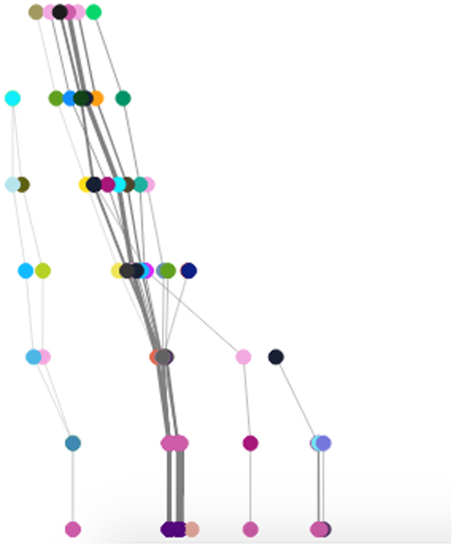
A visualization of “Chloe’s Campaign,” an introductory Prom Week level.

However, it also conveys a certain inertia in the player’s capacity to influence character behavior. One of the intended player experiences of Prom Week is the ability to dynamically influence the desires of the characters through taking actions, but if the same actions are available regardless of the choices the player made, it implies their choices are less important than the starting state baked into the game by its designers. Examining visualizations of other levels confirms this pattern is relegated to this introductory campaign, where it beneficially serves as a forgiving tutorial.

This is exhibited in Figure 8, which depicts a visualization of Doug’s campaign. Here, players begin by pursuing diverse strategies. These strategies largely remain distinct (with one notable exception of one polyline merging into another), though their collective leftward leaning implies some commonality exists across the traces. This is expected behavior for the Prom Week designers, as it implies the game’s players are making choices to satisfy the campaign’s social goals. Traces that lacked this commonality would indicate that Prom Week is capable of accommodating many courses of actions through the game—something of great import to the game’s designers—but that players weren’t motivated by the game’s goals. Here, the analysis reveals distinct paths with similar strategies, which is ideal from the perspective of the game’s designers.

Figure 8.

A visualization of “Doug’s Campaign,” a more complex level than Chloe’s, with additional social goals to achieve.

Finally, Figure 9 depicts two visualizations from a third campaign (Simon). The Prom Week designers have used other visualizations of Simon’s campaign in previous publications³³ to convey the expressive space of their game. As such, it is useful to visualize this data with Gamalyzer as a point of comparison and reference.

Figure 9.

Two visualizations of “Simon’s Campaign.” The top visualization has a pivot count of 10, and the bottom has a pivot count of 20. All other Gamalyzer parameters are consistent across the two.

In previous publications, it was discovered through visualization that every player of Simon’s campaign eventually discovered a path that was uniquely their own. However, prior visualizations made no attempt to communicate how distinct these traces were from each other, nor did they reveal if there were any instances of shared action sequences. It is of great interest to the Prom Week designers to discover if Gamalyzer corroborates the previous findings of trace uniqueness, as well as any additional insight Gamalyzer can offer regarding the relationships the traces have with one another.

When given a pivot count of 10 (the top half of Figure 9), there seem to be a few clusters of similar starting behavior, which tend to spool out into distinct traces. Increasing the pivot count to 20 (the bottom half of the figure) better reveals the range of starting strategies players engaged in. This result agrees with the previously published findings: that some players may begin by taking similar actions to other players, but that gradually these traces become distinct from one another. Additionally, this visualization reveals that there are moments where two mostly distinct paths interweave across one another before separating again. It is surprising to the Prom Week developers that this is possible in a campaign of great length (whereas this behavior was expected and desirable in the much shorter Chloe’s campaign, discussed above), and speaks to the possibility of redundant game states or interchangeable player moves. Knowing that such possibilities exist, the Prom Week designers can analyze these traces to make determinations about what changes—if any—should be made to the game’s simulation system.

Incorporating state visualizations

We have argued that combining action and state visualizations offers novel benefits, filling in weak spots in each family of techniques. This section describes a provisional integration of Playtracer with the Gamalyzer visualization. Because the two tools are built on different user interface platforms, this integration is not automatic and manual cross-indexing of trace identifiers is required; but some modest engineering effort to reproduce either visualization would easily automate this.

We examine a representative analysis task using Playtracer and Gamalyzer in combination for the educational puzzle game Refraction. The theme here is exploratory visualization: at a glance, do we see any surprising strategies or situations?

During exploratory visualization (Figure 10), an analyst might first look at Playtracer to see how many winning states there are, and then at Gamalyzer to see how many groups of action traces there are which end in wins (crosses). If there are more or fewer distinct action sequence groups than there are distinct winning state clusters, this suggests respectively that there are many routes to one or more winning states or that some winning states are very different but can be reached by very similar strategies. We may also look at those traces that do not end in solutions: did the players start out in the right way, or did they make a wrong choice early on that led them astray?

Figure 10.

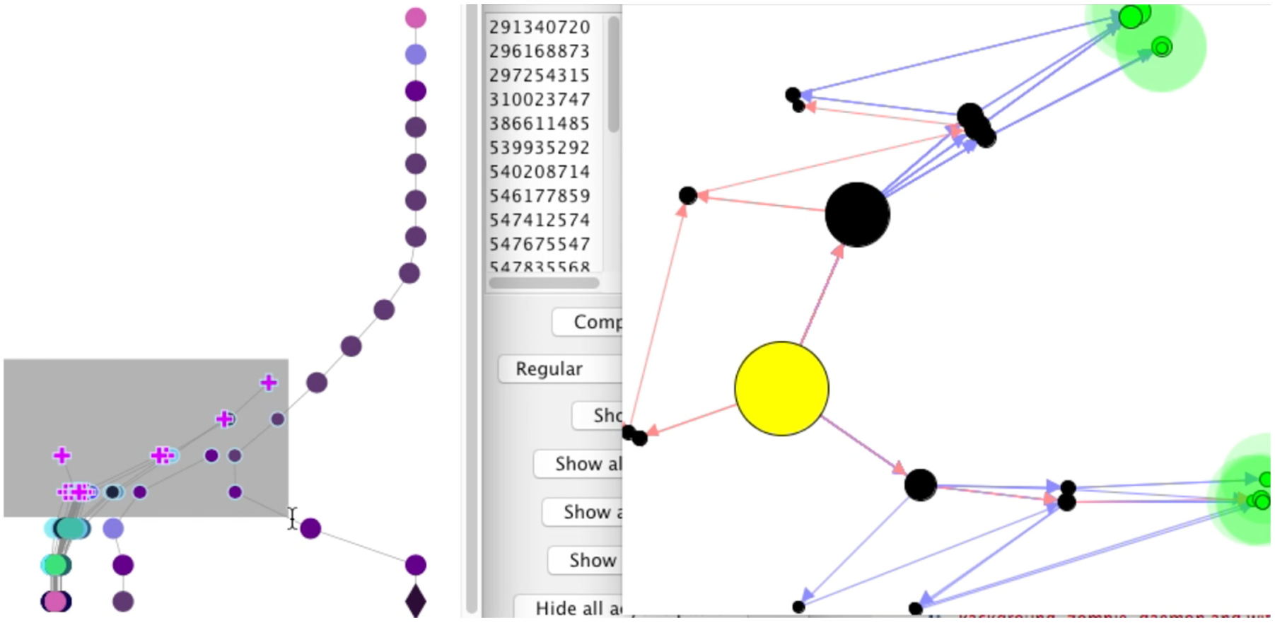
Gamalyzer with Playtracer. Wins are highlighted.

Two interesting facts stand out immediately: First, most of the winning plays are quite similar to each other, even though they result in very different terminal states according to Playtracer—there is a somewhat weak separation between two main groups of the purple crosses (Figure 10). Second, many plays start out in the right direction but never result in a win; this is made clearer by toggling between a high and a low value for s to quickly show the overall and incremental action trace clusterings (Figure 11). Playtracer’s red arrows also show that some players don’t win, but it is difficult to tell quickly how many players or play-throughs are represented by those confused players. Dragging a rectangle over the interesting actions could highlight in Playtracer the states those actions produce (conversely, clicking on a state could show which Gamalyzer traces and actions lead into that state).

Figure 11.

Gamalyzer with Playtracer. Different values of s (0.005 in the top left, 0.002 in the top right, and 0.000 in the bottom left) show overall trends.

Playtracer reveals that there are losing states that are extraordinarily close to winning states, even overlapping in the visualization, but some key property is missing that prevents the win (Figure 12). We can look through the players to see which ones fail to reach the win, and then click on it to see which Gamalyzer trace represents that player. Mousing over that player’s actions and comparing them to their nearest neighbor, we see a series of off-by-one errors from which the player never recovers.

Figure 12.

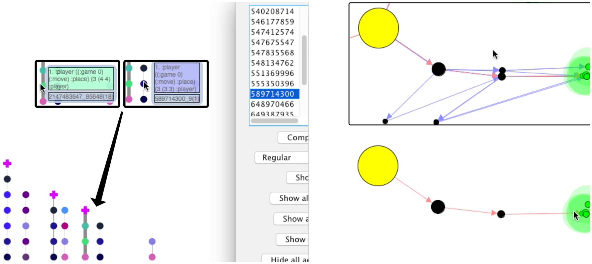
Gamalyzer with Playtracer. An almost-victorious player with a pattern of off-by-one errors (left insets) relative to its closest neighbor. The right inset also shows the proximity of their path to winning paths.

Another interesting aspect of the Gamalyzer visualization is the very long trace on the right: is seems to be just one confused player who picks up and puts down the same piece repeatedly in various nearby positions, eventually giving up (Figure 13). This is not immediately clear from Playtracer, but now that we know what we are looking for we can narrow in on the problematic player and see which states they visited by clicking on the trace. Even though they made many moves, they did not make any significant progress towards any goal. It is interesting that even though syntactically they started to move in the right direction, and they did reach a state that was closer to the goal than their original move, they never made it out of their local minimum.

Figure 13.

Gamalyzer with Playtracer. A player who made many redundant moves (insets) and did not make substantial progress towards any goal.

We can also imagine that the filters provided by Playtracer (all winners, all outliers, etc.) could be shown in Gamalyzer as well, or all the pivots selected by Gamalyzer could be shown in Playtracer. Clicking on a state or an action could show a screenshot of the game in that state, or in a representative state for the cluster. Even generic approaches like these could rapidly accelerate exploratory visualization of game strategy space.

Conclusion

We have presented the Gamalyzer visualization, which lays out gameplay traces to highlight incremental similarities and differences obtained from the Gamalyzer metric (a variant of CCED). Our visualization selects only the most informative (layout-influencing) traces for presentation, optimizing for both computational and visual complexity.

In the future, progressive disclosure could be an extremely useful feature of the interactive visualization: expanding a single exemplar trace into the bundle of traces it represents, their layout bounded within a portion of the image could act like a loupe or callout to more closely inspect a subset of traces. Displays which allow dilation of time to illustrate sequence alignments could also help understand similarities between traces. We would also like to experiment with three-dimensional views to better separate traces at each time slice.

Selecting an appropriate encoding for Gamalyzer remains a bit of an art, but this article provides guidelines for analysts. Of course, the option remains to use a custom action distance function, but we feel that the weighted lexicographic order solves more problems than it creates (and remains simpler than defining a game-specific state-distance measure).

While we have informally used Gamalyzer in concert with Playtracer, we believe that formally integrating the two systems (potentially also incorporating Glyph as well as screenshots of the games as they are played) could lead to an extremely useful multimodal analysis platform—perhaps a game-specialized analog to VisTrails.⁴¹

Footnotes

Funding

The author(s) received no financial support for the research, authorship, and/or publication of this article.

References

Osborn

Mateas

. A game-independent play trace dissimilarity metric. In: Proceedings of the 9th international conference on the foundations of digital games, Fort Lauderdale, FL, 3–7 April 2014.

Zook

Harrison

Riedl

. Monte-Carlo tree search for simulation-based strategy analysis. In: Proceedings of the 10th conference on the foundations of digital games, Pacific Grove, CA, 22–25 June 2015.

Chhieng

Wong

. Adaptive distance measurement for time series databases. In: Kotagiri

Krishna

Mohania

. (eds) Advances in databases: concepts, systems and applications. Berlin; Heidelberg: Springer, 2007, pp. 598–610.

Osborn

Samuel

McCoy

. Evaluating play trace (dis)similarity metrics. In: Proceedings of the 10th annual AAAI conference on artificial intelligence and interactive digital entertainment, Raleigh, NC, 3–7 October 2014.

Gaudl

Osborn

Bryson

. Learning from play: facilitating character design through genetic programming and human mimicry. In: Pereira

Machado

Costa

. (eds) Portuguese conference on artificial intelligence. Cham: Springer, 2015, pp. 292–297.

Moura

El Nasr

Shaw

. Visualizing and understanding players’ behavior in video games: discovering patterns and supporting aggregation and comparison. In: Proceedings of the 2011 ACM SIGGRAPH symposium on video games, Vancouver, BC, Canada, 10 August 2011, p. 2. New York: ACM.

El Nasr

Drachen

Canossa

Game analytics: maximizing the value of player data. London: Springer, 2013.

Andersen

Liu

Apter

. Gameplay analysis through state projection. In: Proceedings of the 5th international conference on the foundations of digital games, Monterey, CA, 19–21 June 2010, pp. 1–8. New York: ACM.

Wallner

Kriglstein

. A spatiotemporal visualization approach for the analysis of gameplay data. In: Proceedings of the SIGCHI conference on human factors in computing systems (CHI’12), Austin, TX, 5–10 May 2012, pp. 1115–1124. New York: ACM.

10.

Nguyen

THD

El-Nasr

Canossa

. Glyph: visualization tool for understanding problem solving strategies in puzzle games. In: Proceedings of the 10th conference on the foundations of digital games, Pacific Grove, CA, 22–25 June 2015.

11.

Raphaël

Gareth

Pierre

. Understanding player experience through the use of similarity matrix. In: Proceedings of the 2015 DiGRA international conference (DiGRA ’15), Lüneburg, 14–17 May 2015. Tampere, Finland: Digital Games Research Association, http://www.digra.org/digital-library/

12.

Thawonmas

Iizuka

. Visualization of online-game players based on their action behaviors. Int J Comput Game Technol 2008; 2008: 5.

13.

Loh

Sheng

. Measuring the (dis-)similarity between expert and novice behaviors as serious games analytics. Educ Inform Tech 2015; 20(1): 5–19.

14.

Kohwalter

Clua

Murta

. Game flux analysis with provenance. In: Reidsma

Katayose

Nijholt

(eds) Advances in computer entertainment. Cham: Springer, 2013, pp. 320–331.

15.

Wender

Cordier

Watson

. Building a trace-based system for real-time strategy game traces. In: Proceedings of the EXPPORT: EXperience reuse: provenance, process-ORientation and traces (ICCBR), Case-Based-Reasoning Saratoga Springs, NY, 8–11 July 2013, pp. 1–10. Menlo Park, CA: AAAI Press.

16.

Sali

Mateas

. Using information visualization to understand interactive narrative: a case study on façade. In: Proceedings of the international conference on interactive digital storytelling, Vancouver, BC, Canada, 28 November–1 December 2011, pp. 284–289. London: Springer.

17.

Sali

Wardrip-Fruin

Dow

. Playing with words: from intuition to evaluation of game dialogue interfaces. In: Proceedings of the 5th international conference on the foundations of digital games, Monterey, CA, 19–21 June 2010, pp. 179–186. New York: ACM.

18.

Wongsuphasawa

Alexis

Gomez

. LifeFlow: visualizing an overview of event sequences. In: Proceedings of the SIGCHI conference on human factors in computing systems, 2011, pp. 1747–1756. ACM.

19.

Tremblay

Torres

Rikovitch

. An exploration tool for predicting stealthy behaviour. Technical Report WS-11-19. In: Proceedings of the 2nd workshop on artificial intelligence in the game design process, Boston, MA, 15 October 2013, pp. 1–7. Menlo Park, California: AAAI Press.

20.

Ortega

Shaker

Togelius

. Imitating human playing styles in Super Mario Bros. Entertain Comput 2013; 4(2): 93–104.

21.

Smyth

. Clustering sequences with hidden Markov models. In: Mozer

Jordan

Petsche

(eds) Advances in neural information processing systems. Cambridge, MA: MIT Press, 1997, pp. 648–654.

22.

Karakovskiy

Togelius

. The Mario Ai Benchmark and competitions. IEEE T Comp Intel AI 2012; 4(1): 55–67.

23.

Shaker

Yannakakis

Togelius

. Crowdsourcing the aesthetics of platform games. IEEE T Comp Intel AI 2013; 5: 276–290.

24.

Algorithmics Group. MDSJ: Java library for multidimensional scaling (version 0.2). 2009, http://www.inf.uni-konstanz.de/algo/software/mdsj/

25.

Bostock M. d3.js data-driven documents, 2011, http://vis.stanford.edu/files/2011-D3-InfoVis.pdf

26.

Brandes

Pich

. Eigensolver methods for progressive multidimensional scaling of large data. In: Kaufmann

Wagner

(eds) Graph drawing (Lecture notes in computer science), vol. 4372. Berlin; Heidelberg: Springer, 2007, pp. 42–53.

27.

Leslie

Eskin

Cohen

. Mismatch string kernels for discriminative protein classification. Bioinformatics 2004; 20(4): 467–476.

28.

Sakoe

Chiba

. Dynamic programming algorithm optimization for spoken word recognition. IEEE T Acoust Speech 1978; 26(1): 43–49.

29.

Itakura

. Minimum prediction residual principle applied to speech recognition. IEEE T Acoust Speech 1975; 23(1): 67–72.

30.

Chowdhury

Ramachandran

. Cache-oblivious dynamic programming. In: Proceedings of the 17th annual ACM-SIAM symposium on discrete algorithm, Miami, FL, 22–26 January 2006, pp. 591–600. Philadelphia, PA: Society for Industrial and Applied Mathematics.

31.

Holmgård

Togelius

Yannakakis

. Decision making styles as deviation from rational action: a Super Mario case study. In: Proceedings of the AAAI conference on artificial intelligence and interactive digital entertainment, Boston, MA, 14–18 October 2013.

32.

McCoy

Treanor

Samuel

. Prom week: designing past the game/story dilemma. In: Proceedings of the 8th international conference on the foundations of digital games FDG 2013, Chania, Crete, Greece, 14–17 May 2013.

33.

McCoy

Treanor

Samuel

. Social story worlds with Comme il Faut. IEEE T Comp Intel AI 2014; 6: 97–112.

34.

Samuel

McCoy

Treanor

. Story sampling: a new approach to evaluating and authoring interactive narrative. In: Proceedings of the 9th international conference on the foundations of digital games, Fort Lauderdale, FL, 3–7 April 2014.

35.

Hickey

. Extensible data notation, 2012, https://github.com/edn-format/edn

36.

Liapis

Yannakakis

Togelius

. Designer modeling for personalized game content creation tools. In: Proceedings of the AAAI conference on artificial intelligence and interactive digital entertainment, Boston, MA, 14 October 2013.

37.

Vinh

Epps

Bailey

. Information theoretic measures for clusterings comparison: variants, properties, normalization and correction for chance. J Mach Learn Res 2010; 11: 2837–2854.

38.

Rogowitz

Frese

Smith

. Perceptual image similarity experiments. In: Proceedings of the human vision and electronic imaging III, San Jose, CA, 24 January 1998, vol. 3299, pp. 576–590. Bellingham, WA: International Society for Optics and Photonics.

39.

Russell

Sinha

. A perceptually based comparison of image similarity metrics. Perception 2011; 40(11): 1269–1281.

40.

McCoy

Mateas

. All the world’s a stage: a playable model of social interaction inspired by dramaturgical analysis. PhD Thesis, University of California—Santa Cruz, Santa Cruz, CA, 2012.

41.

Bavoil

Callahan

Crossno

. VisTrails: enabling interactive multiple-view visualizations. In: Proceedings of the IEEE Visualization (VIS 05), Minneapolis, MN, 23–28 October 2005, pp. 135–142. New York: IEEE.