Visual feature fusion and its application to support unsupervised clustering tasks

Introduction

Machine learning and data mining techniques are, in general, split into supervised and unsupervised approaches or a combination of both. In supervised approaches, user knowledge can be input into the analytical process through sets of processed data instances. In unsupervised, knowledge can be added by changing algorithm parameters or the data representation, also known as features. For unsupervised methods, therefore, the challenge is not only to define the most appropriate set of parameters but also to find the data representation that best expresses user knowledge or expectation.

Depending on the application domain (e.g. text or image), there exist several approaches to constructing features, each providing complementary information about the original or raw data. Since there is no perfect feature, the idea of joining different representations is straightforward. This process is called data or feature fusion, ¹ and it can occur through combining the features’ vector representation or merging distances calculated from them. When the machine learning or data mining task involves a cost function, for instance, classification accuracy, it can be used to guide the combination. However, for tasks, like clustering^2,3 or multidimensional projection,^4,5 where such a function does not exist, support needs to be provided to allow users to build proper combinations. Otherwise, in practice, data fusion is impossible or useless given the abundance of possible combinations.

In this article, we present a novel feature fusion approach that allows users to control and understand the fusion of different feature sets. Starting with a small sample, users employ a simple widget to define the weights for the combination and observe in real-time the outcome through a scatterplot-based visualization. Once users find the weighted combination that best matches their point of view of similarity, the same weights can be used to combine the complete data set. In this way, we not only allow users to test different combinations easily but also enable the interpretation of the attained results.

In summary, the main contributions of this article are the following:

Related work

The process of integrating information from multiple sources to produce a unified enhanced data model is called data fusion. ¹ The goal is to combine different data representations into a single model aimed at incorporating properties from various sources. Data fusion can occur in different ways, including combining features, that is, the vectorial data representation, or merging distances calculated from the various sources.

The concept of merging features is called feature fusion. Feature fusion aims to generate a unified vectorial data representation based on different sets of features (vectorial representations).^6,7 The most straightforward approach is feature concatenation.^8,9 In concatenation, given the sets of features F 1 , F 2 , … , F p , the unified representation is given by [ F 1 , F 2 , … , F p ] . Despite its simplicity, the literature reports several examples. In Wang et al., ¹⁰ Local Binary Pattern (LBP) ¹¹ and Histograms of Oriented Gradients (HOGs) ¹² features are concatenated to improve performance in pedestrian detection. In Manshor et al., ¹³ Scale Invariant Transform Features (SIFT) ¹⁴ and boundary-based shape ¹⁵ features are concatenated to improve object recognition. In Chu et al., ¹⁶ high, low, and medium layer features of a deep neural network are united to support object detection, and in Chun et al., ¹⁷ color and texture features are progressively concatenated to reduce model complexity in a content-based retrieval framework. Feature concatenation has also been used in the text domain. In Loni et al., ¹⁸ the authors extract seven types of lexical, syntactical, and semantic features and combine subsets of them to improve text classification.

Weights can be used in the concatenation process to control the influence of the different features. In this process, the unified representation is given by [ α 1 F 1 , α 2 F 2 , … , α p F p ] , ⁶ where α 1 , α 2 , … , α p are the weights. In Loni et al., ¹⁹ a weighted concatenation was used to improve text classification by combining lexical, syntactic, and semantic features. In Ma et al., ²⁰ a neural network was used to learn the weights of a concatenation, combining different image features, such as color, shape, and texture, to improve classification accuracy. In You and Tang, ²¹ the authors use a saliency detection model to fuse color and texture features through a weighting strategy. First color and texture features are transformed into saliency features, which are then combined linearly. Different from the previous weighted techniques, features are combined instead of concatenated, that is, the unified representation is given by [ α 1 F 1 + α 2 F 2 + … + α p F p ] . Such combination is possible since the saliency representations have the same dimensionality.

In practice, the feature concatenation is not recommended since it may result in high-dimensional feature vectors leading to the curse of dimensionality problem. ⁶ One solution is to apply a dimensionality reduction after the concatenation, ²² or to perform a distance fusion. In the distance fusion, instead of combining the vectorial representations, the distances calculated from the representations are combined. If Δ ( F i ) represents the distance matrix calculated from F i , the resulting distance matrix is given by α 1 Δ ( F 1 ) + α 2 Δ ( F 2 ) + … + α p Δ ( F p ) . In Degani et al., ²³ a simple normalized combination of distances computed from different types of features is used to cover song identification. The distance fusion can also be performed using weights. In Huang et al., ²⁴ weights are used to combine distances calculated from color and texture features to improve the results of a content-based image retrieval system. In Vadivel et al., ²⁵ distances calculated from color and texture features are also combined to support content-based image retrieval applications. Finally, in Liu et al. ²⁶ and in Chu et al., ¹⁶ distances calculated from features extracted from different layers of a deep neural network are combined to improve retrieval tasks.

Different from data fusion, model fusion combines computational models instead of data. Such combination can be performed in two different ways: by combining different models (parametrizations) processing a single feature set (data set), or by combining different models processing different feature sets. ²⁷ The former is called ensemble learning and has been extensively used in classification tasks. The idea is to combine the predictions from different models using a voting strategy to improve model diversity and classification accuracy.^28,29 Ensembles of classifiers typically outperform single classifiers ³⁰ and have been used in different domains, including remote sensing, computer security, financial risk assessment, fraud detection, recommender systems, medical computer-aided diagnosis, and others.^27,31 Similarly, the later also employs a (weighted) voting strategy to combine different models, but in this case, the models use different sets of features as input. Examples of applications include fruit classification ⁹ and sentiment analysis. ³²

Common to all these data and model fusion approaches is that combinations can only be performed when a loss function is available to guide the process, like in classification. If such a function does not exist, or there is a degree of subjectivity in the process, the combination without proper user support hampers its applicability in practice or real scenarios, and none of the mentioned approaches offer such support. In this article, we devise an approach to aid the process of feature combination to allow users to control the process to match individual expectations, enabling applications where user judgment is crucial.

Proposed methodology

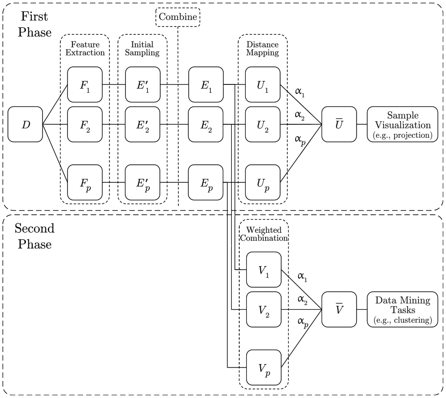
Our feature fusion approach employs a two-phase strategy to support users to define combinations that reflect a particular point-of-view regarding similarity. Considering an original or raw data set D = { d 1 , d 2 , … , d n } with n elements (e.g. an image collection), and F 1 = { f 1 1 , … , f n 1 } , … , F p = { f 1 p , … , f n p } the different sets of feature vectors extracted from D . In the first phase of our approach, initial sample sets E ′ 1 , E ′ 2 , … , E ′ p are selected from each different set of feature vectors, and the indexes of these vectors are merged to compose a single list of indexes containing all elements captured by the different samplings. After that, new sample sets E 1 , E 2 , … , E p are built containing the different types of feature vectors. They represent the same elements given by this common list of indexes so that all sample sets have the same number of elements q , that is, q = | E 1 | = | E 2 | = … = | E p | . Each sample E i is then mapped to a vectorial representation U i = { u 1 i , u 2 i , … , u q i } ∈ R m preserving as much as possible the distance relationships, and these representations are combined to generate a single representation U ¯ = α 1 U 1 + α 2 U 2 + … + α p U p , which is then visualized.

The user can then change the feature weights α 1 , α 2 , … , α p and observe the resulting combination in real-time. Once the sample visualization reflects the user expectations, that is, once proper feature weights are found, the second phase takes place, and these weights are used to combine the complete set of features F 1 , F 2 , … , F p . In this process, the mapped sample representations U 1 , U 2 , … , U p and the samples E 1 , E 2 , … , E p are used to construct models to transform each set of feature F i to a vectorial representation V i ∈ R m . Since these vectorial representations are embedded in the same space, they can be combined using the weights α 1 , α 2 , … , α p , obtaining the final vectorial representation V ¯ = α 1 V 1 + α 2 V 2 + … + α p V p that seeks to match the user expectations defined by the sample visualization. Figure 1 outlines our approach showing the involved steps. Next, we detail these steps, starting with the sampling and the distance preservation mapping.

OPEN IN VIEWER

Figure 1.

Overview of our feature fusion process. Initially, a sample is extracted, combined, and visualized. Based on this, the user can test different weights to fuse the features and observe the outcome. Once a sample combination that reflects the user expectation is found, the same weights are used to combine the complete sets of features that can then be used on subsequent data mining tasks, such as clustering.

Sampling and mapping

The first step of our process is sampling. Since users employ the sample visualization to guide the feature fusion process, it is essential to have all possible data patterns from the different features represented. Therefore, we recover samples from each different set of features so as to represent the distribution of each set faithfully.

In this process, we extract samples from each set F 1 , F 2 , … , F p independently using a cluster-based strategy. We employ the k-means algorithm to create n clusters, getting the medoid of each cluster as a sample, where n is the number of instances in the raw data set D . We set the number of clusters to n since this is considered a useful heuristic for the upper-bound number of clusters in a data set. ³³ As explained, after extracting the sample sets E ′ 1 , E ′ 2 , … , E ′ p , we merge their indexes to define a unified set of indexes, and create the sets E 1 , E 2 , … , E p having feature vectors with the indexes contained in the unified set of indexes. This is an essential and mandatory step since the sample visualization is constructed based on the combination of all features, and this combination is only possible to compute if the samples contain vectors representing the same data elements. Also, this increases the chance of representing the different patterns contained in the different sets of features. Notice that the combined sample features U ¯ will have at most n × p instances, enhancing the probability of having samples that represent the distribution and patterns of each set of features while not hampering the computational complexity of the overall process since p << n .

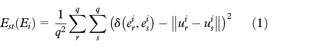
After recovering the samples, we map them to a common m -dimensional space, obtaining their vectorial representation U 1 , U 2 , … , U p ∈ R m so that we can combine them to obtain U ¯ ∈ R m (for the sample visualization). In this process, each set of samples E i is mapped to R m preserving as much as possible the distance relationships. We do this by minimizing

E st ( E i ) = 1 q 2 ∑ r q ∑ s q ( δ ( e r i , e s i ) − ‖ u r i − u s i ‖ ) 2

(1)

where e r i and e s i are feature vectors in E i , δ ( e r i , e s i ) is the distance between them, and u r i and u s i are the vectorial representations in the m -dimensional space of e r i and e s i , respectively.

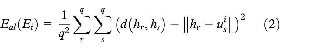
Besides preserving distance relationships, our mapping process aims to align the vectorial representations so that u r i is placed as close as possible to u r j ∀ j ∈ [ 1 , p ] , r ∈ [ 1 , q ] without affecting the distance preservation of the individual mappings. This is necessary since the unified sample representation is calculated as a convex combination of these representations, that is, U ¯ = α 1 U 1 , α 2 U 2 , … , α p U p , with ∑ α i = 1 , and misalignments could result in meaningless unified representations. First, we calculate the average distance matrix Δ ¯ = ( 1 / p ) ∑ i p Δ ( E i ) by combining the distance matrices of all set of samples, where Δ ( E i ) = ( δ rs = δ ( e r i , e s i ) ) is the distance matrix calculated from E i . Then we map Δ ¯ to the m -dimensional space using equation (1) but replacing δ ( e r i , e s i ) by δ rs obtaining H ¯ = { h ¯ 1 , h ¯ 2 , … , h ¯ q } ∈ R m . The idea is to use this average vectorial representation as a guide to align the vectorial representations U 1 , U 2 , … , U p minimizing

E al ( E i ) = 1 q 2 ∑ r q ∑ s q ( d ( h ¯ r , h ¯ s ) − ‖ h ¯ r − u s i ‖ ) 2

(2)

where d ( h ¯ r , h ¯ s ) is the distance between two instances of the average vectorial representation.

Joining equations (1) and (2) renders the function we optimize in our mapping process seeking to preserve, as much as possible, the distance relationships of the sample set of features E 1 , E 2 , … , E p in the vectorial representations U 1 , U 2 , … , U p ∈ R m while aligning them. This function is given by

E mapping ( E i ) = λ · E st ( E i ) + ( 1 − λ ) · E al ( E i )

(3)

where λ is used to control the importance of the distance preservation and the alignment to the produced vectorial representations. λ is a hyperparameter and can be changed to define a good trade-off between distance preservation and alignment.

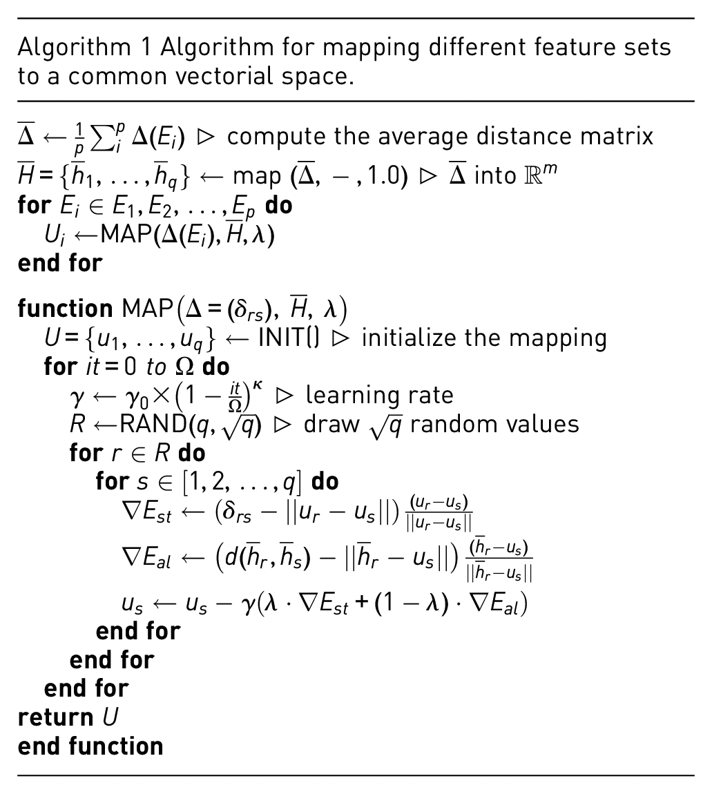
To minimize equation (3), we use a stochastic gradient descent approach with a polynomial decay learning rate. We set the initial learning rate to γ 0 = 0 . 1 , the decay power to κ = 0 . 95 , and the number of iterations Ω = 100 , following common choices found in the literature. ³⁴ Algorithm 1 outlines our mapping process. Function RAND ( t , k ) randomly draws k discrete values in the range [ 1 , 2 , … , t ] , and function INIT ( ) initializes the mapping coordinates, also randomly. We tested a deterministic initialization using Fastmap, ³⁵ but the gain in quality does not justify the computational overhead. Also, the first time the function MAP ( … ) is called, H ¯ is not provided. In this case, ∇ E al is not computed and only ∇ E st is considered to calculate the mapping coordinates.

Notice that we normalize all features f i ∈ F j , ∀ i , j before this process, so that the Euclidean norm | | f i | | = 1 . Given the triangular inequality property ( | | f i − f j | | ≤ | | f i | | + | | f j | | ) , this guarantees a upper limit for the maximum pairwise distance between features. Therefore, the distances are in the same range despite the type of feature or its dimensionality, avoiding biasing the process toward the type of feature with the largest maximum distance. In addition, we define the dimensionality m of the resulting mappings U 1 , U 2 , … , U p ∈ R m as the largest intrinsic dimensionality of F 1 , F 2 , … , F p , calculated using the maximum likelihood estimation. ³⁶ Such dimensionality can also be defined by the user if the target dimensionality is known, such as m = { 1 , 2 , 3 } for visualization purposes.

OPEN IN VIEWER

Algorithm 1 Algorithm for mapping different feature sets to a common vectorial space.

Δ ¯ ← 1 p ∑ i p Δ ( E i ) ▹ compute the average distance matrix H ¯ = { h ¯ 1 , … , h ¯ q } ← map ( Δ ¯ , − , 1 . 0 ) ▹ Δ ¯ into R m for E i ∈ E 1 , E 2 , … , E p do   U i ← MAP ( Δ ( E i ) , H ¯ , λ ) end for functionMAP ( Δ = ( δ rs ) , H ¯ , λ )   U = { u 1 , … , u q } ← INIT() ▹ initialize the mapping  for it = 0 to Ω do    γ ← γ 0 × ( 1 − it Ω ) κ ▹ learning rate    R ← RAND ( q , q ) ▹ draw q random values   for r ∈ R do    for s ∈ [ 1 , 2 , … , q ] do      ∇ E st ← ( δ rs − | | u r − u s | | ) ( u r − u s ) | | u r − u s | |      ∇ E al ← ( d ( h ¯ r , h ¯ s ) − | | h ¯ r − u s | | ) ( h ¯ r − u s ) | | h ¯ r − u s | |      u s ← u s − γ ( λ · ∇ E st + ( 1 − λ ) · ∇ E al )    end for   end for  end for return U end function

Weighted feature combination

Given the sample vectorial representations U 1 , U 2 , … , U p , we build a set of functions using the process defined in Joia et al. ³⁷ to map each feature set F i into its vectorial representation V i ∈ R m preserving as much as possible the distance relationships while obeying the geometry defined in U i . In this process, each instance f j i ∈ F i is mapped to the m -dimensional space through an orthogonal local affine transformation T j i : R m i → R m , where m i is the dimensionality of F i .

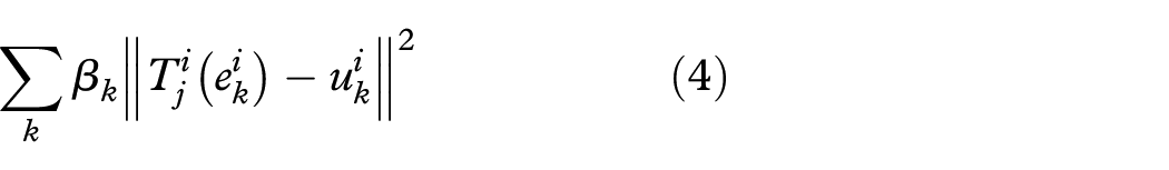
The affine transformation T j i ( f ) = fM + t associated with f j i is defined so as to minimize

∑ k β k ‖ T j i ( e k i ) − u k i ‖ 2

(4)

where β k = ∥ e k i − f k i ∥ − 2 , with e k i the original feature representation of the kth sample in E i .

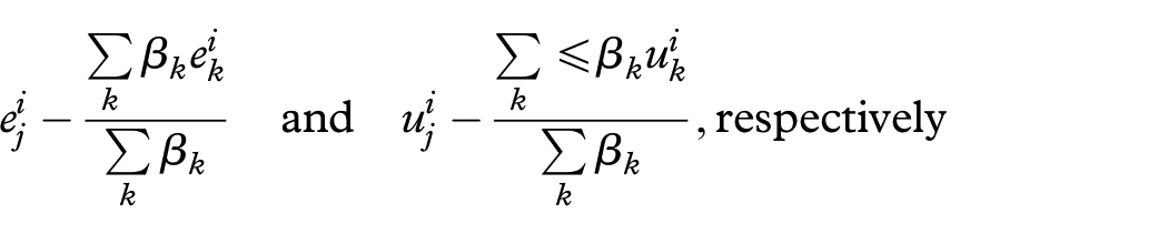
Equation (4) can be re-written in the matrix form ∥ C ( AM − B ) ∥ F , where ∥ · ∥ F denotes the Frobenius norm, C is a diagonal matrix with entries C ii = β i , and A and B are matrices with the jth row given by the vectors

e j i − ∑ k β k e k i ∑ k β k and u j i − ∑ k ≤ β k u k i ∑ k β k , respectively

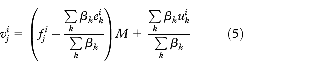
Based on that, M is computed as M = SR , where S and R are obtained from the singular value decomposition of A T CCB = ST R T . Then, the vectorial representation v j i of f j i is given by

v j i = ( f j i − ∑ k β k e k i ∑ k β k ) M + ∑ k β k u k i ∑ k β k

(5)

Equation (4) is subject to M M ⊤ = I , which avoids scale and shearing effects, therefore, preserving the distance relationships of the input features. Also, notice that the sample vectorial representations U 1 , U 2 , … , U p dictate the geometry of the embeddings V 1 , V 2 , … , V p . Since they are aligned by the mapping process defined in the previous section, the linear combination V ¯ = α 1 V 1 , α 2 V 2 , … , α p V p can be performed to obtain the final embedding V ¯ . That incorporates the patterns defined by each set of features, weighted according to the user’s point-of-view. For more information about this affine transformation and how the sample vectorial representation controls the final results, please refer to Joia et al. ³⁷

Feature combination widget

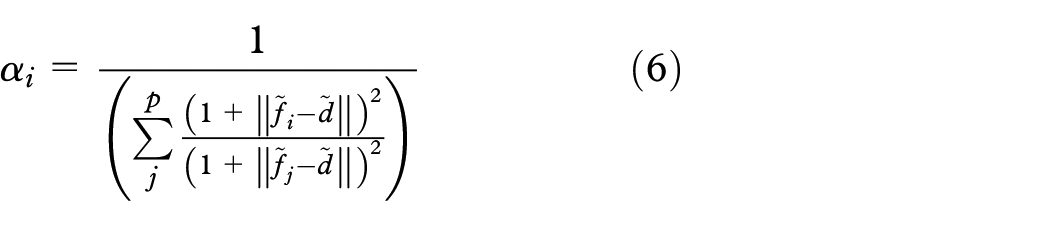
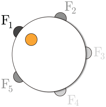
To support the feature sample combination, we create a widget inspired by the strategy presented in Pagliosa et al. ³⁸ The idea is to position anchors (circles) representing each different set of features on a circumference, computing the weights α 1 , α 2 , … , α p according to their distances to a “dial,” which can be freely manipulated by the user, contained in the circumference. If f ~ i are the coordinates of the anchor representing the feature F i and d ~ the coordinates of the “dial,” the weight α i related to F i is calculated as

α i = 1 ( ∑ j p ( 1 + ‖ f ~ i − d ~ ‖ ) 2 ( 1 + ‖ f ~ j − d ~ ‖ ) 2 )

(6)

Initially, the anchors are equally spaced on the circumference following a random order. However, users can freely move them to produce the desired combinations. Also, to help the perception of the weights, we set the transparency level of the anchors and fonts according to α 1 , α 2 , … , α p . Figure 2 shows the combination widget. In this example, the “dial” in orange is closer to the anchor representing the feature F 1 , so the corresponding anchor is more opaque than the others.

OPEN IN VIEWER

Figure 2.

Feature combination widget. Using the orange “dial,” users can control the contributions of the different types of features for the final feature combination.

In addition to this design, we have explored another option using multiple sliders, one per feature. Although sliders are commonly used in applications that involve setting multiple parameters, it proved to not be the best choice in our combination scenario. Given that changes in one slider affect the others (it is a convex combination), every user interaction requires adjusting several sliders at once. In our design, users need to manipulate only one dial (and optionally the anchors), providing a much faster exploratory process.

Results and evaluation

In this section, we evaluate our mapping and feature combination processes using different data sets in order to show that the sample manipulation effectively controls the complete feature fusion. Next, we describe the employed data sets, detail how we extract features, and present our quantitative and qualitative evaluation.

Data sets

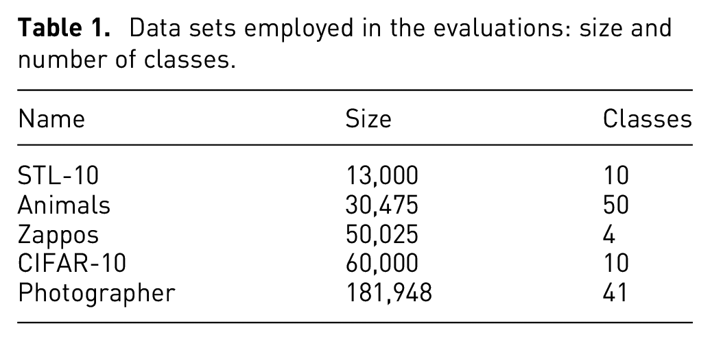
We use five data sets in our tests, named STL-10, ³⁹ Animals, ⁴⁰ Zappos, ⁴¹ CIFAR-10, ⁴² and Photographers. ⁴³ These data sets come from a variety of different domains. The STL-10 consists of 13 , 000 images split into 10 classes of different objects. Similarly, CIFAR-10 contains 60 , 000 images from 10 commonly seen object categories (e.g. animals, vehicles, and so on) in lower resolution. The Animals data set is more specific and it is composed of 30 , 475 images of animals in 50 categories. Zappos is a data set for shoes with 50 , 025 images from Zappos.com split into 4 shoe categories. Finally, the Photographers consists of 181 , 948 photos taken by 41 well-known photographers. Table 1 summarizes the data sets, showing the number of instances and classes.

OPEN IN VIEWER

Table 1.

Data sets employed in the evaluations: size and number of classes.

Name	Size	Classes
STL-10	13,000	10
Animals	30,475	50
Zappos	50,025	4
CIFAR-10	60,000	10
Photographer	181,948	41

Quantitative evaluation

To confirm the quality of our approach, we quantitatively evaluate our mapping and feature combination processes. For the mapping process evaluation, the five data sets of Table 1 are randomly sampled 10 times, reducing them to 5 % of their original sizes. We sample the data since we cannot execute the mapping process on large data sets given its memory footprint of O ( n 2 ) . Due to the random initialization (see Algorithm 1), we repeat the mapping process test 15 times. Moreover, to ensure a common dimensional space, we calculate the intrinsic dimensionality of each set of features and choose the smallest value. This value is used to do the mapping. The minimum values of intrinsic dimensionality are 57 , 71 , 91 , 41 , and 83 for STL-10, Animals, Zappos, CIFAR-10, and Photographer data sets, respectively.

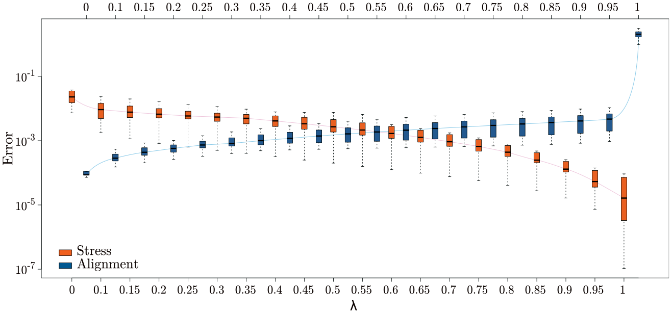
We use stress and alignment error to evaluate the mapping process (see equations (1) and (2), respectively). We summarize our results in Figure 3 varying the value of λ in the range [ 0 , 1 ] . The stress boxplots (in orange) decrease as λ increases whereas the alignment boxplots (in blue) have the opposite behavior. This is the expected outcome since larger values of λ preserve the distance relationships, and smaller values align the data.

OPEN IN VIEWER

Figure 3.

Comparing distance preservation versus alignment error with varying λ . The best trade-off is achieved in the range [ 0 . 45 , 0 . 65 ] . The blue and orange lines connect the average values of the boxplots.

Setting λ = 1 preserves as much as possible the original distance relationships. This is reflected by the average stress E st ¯ = 0 . 0009 , but it does not ensure any alignment ( E al ¯ = 2 . 0343 ) . On the contrary, λ = 0 delivered almost a perfect alignment ( E al ¯ = 0 . 0001 ) , but it does not enforce the distance preservation ( E st ¯ = 0 . 0345 ) . In this article, we are interested in the best trade-off between distance preservation and alignment so that the alignment is obtained without penalizing the overall distance preservation. According to our experiments, we achieved this in the range λ = [ 0 . 45 , 0 . 65 ] , where both stress and alignment errors are nearly 0 for our experiments (see Figure 3).

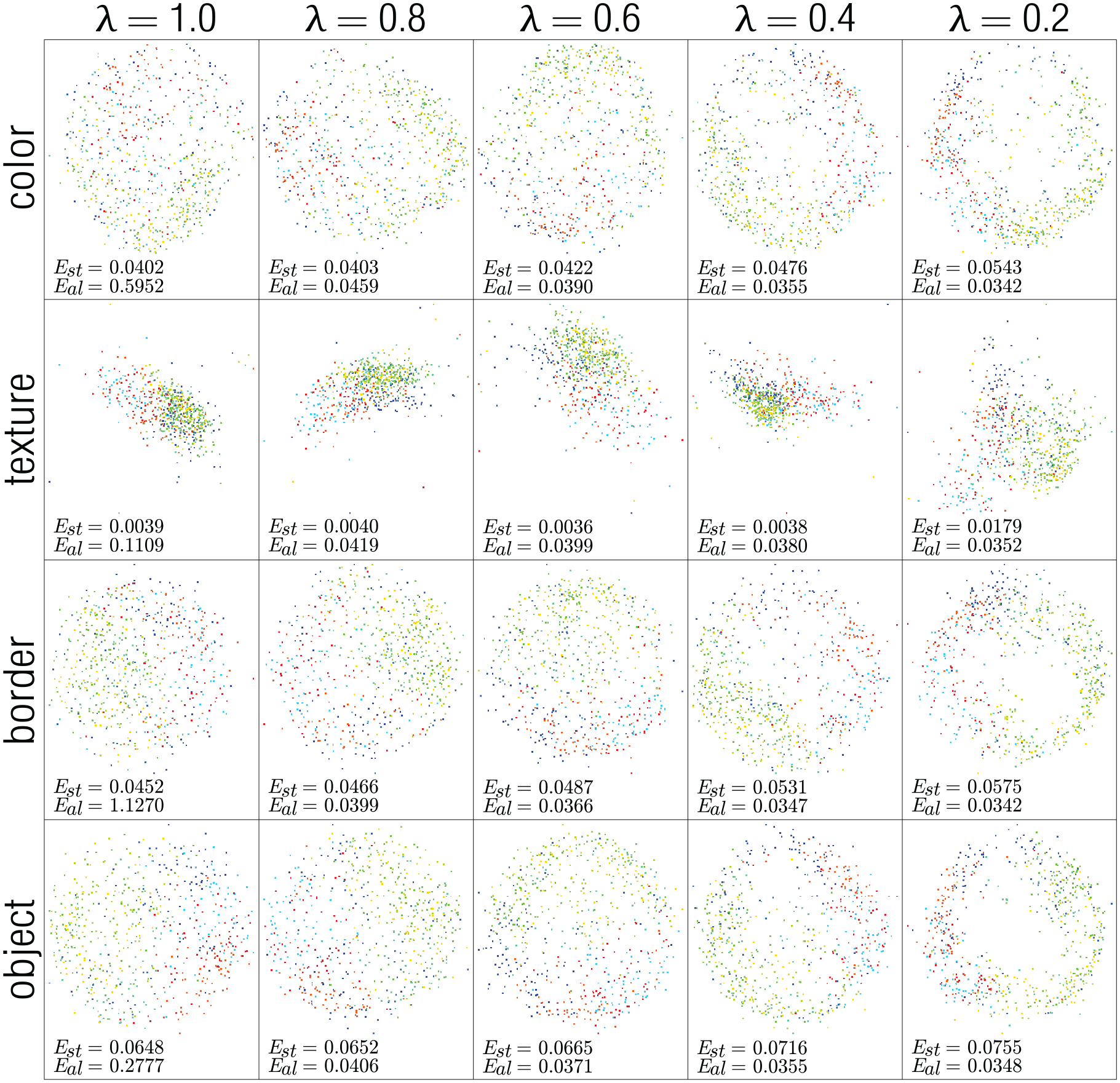
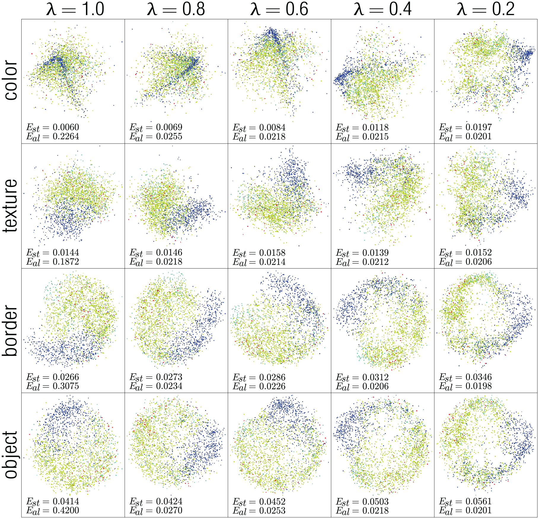
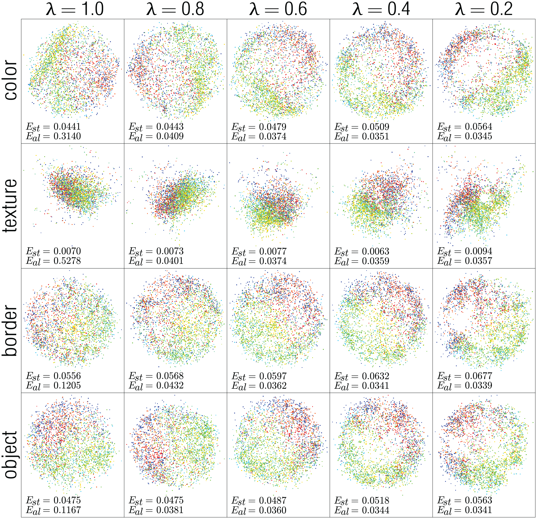
For visual inspection, we map the samples setting the target dimensionality to two. We show the results for the STL-10, Zappos, and CIFAR-10 data sets in Figures 4 –6, respectively. In these figures, the points are colored according to image class. The stress and alignment error values are shown at the bottom-left corner of each projection. To show the influence of λ values in the mapping process, we vary λ in the range [ 1 . 0 , 0 . 2 ] . Notice that in the first column of all figures, the visual representations of each feature (color, texture, border, and object) are misaligned among themselves. That is, points belonging to the same class are placed in different regions on the different projections. For instance, in the first column of Figure 4, the points colored in green are positioned at the bottom in the projection of the color features, on the right in the projection of texture features, and on the left in the projections of the border and object features. The second column depicts results with λ = 0 . 8 . The projections start to align, and points belonging to the same class are placed in similar regions across the different projections. We observe a small increase in the stress error, but the alignment error decreases considerably compared with the first column (see the E al measure at the bottom-left corner). The same behavior is observed in the remaining columns. As expected, as lambda decreases, the alignment improves (alignment error decreases), and the distance preservation decreases (stress error increases). However, the stress changes are minimal, showing that our approach is capable of aligning different feature spaces while preserving the distance relationships in them.

OPEN IN VIEWER

Figure 4.

Resulting 2D mapping process for the STL-10 data set. As λ decreases, the features get more aligned (see last column). Bottom-left numbers correspond to stress and alignment error.

OPEN IN VIEWER

Figure 5.

Resulting 2D mapping process for the Zappos data set. As λ decreases, the features get more aligned (see last column). Bottom-left numbers correspond to stress and alignment error.

OPEN IN VIEWER

Figure 6.

Resulting 2D mapping process for the CIFAR data set. As λ decreases, the features get more aligned (see last column). Bottom-left numbers correspond to stress and alignment error.

For the feature combination, we assess the degree that the distance relationships of the sample are preserved in the feature fusion of the whole data set, intending to demonstrate the effectiveness of the user sample manipulation on the produced data set. In this evaluation, we first randomly generate 30 different weight combinations summing up to 1 and apply them to the sample data. Then, we reuse these weights for the whole data fusion and measure if the distance relationships induced by the weights on the sample are preserved in the whole data set. We use the Nearest Neighbor Measure (NNM) ⁴⁶ to evaluate the degree of preservation.

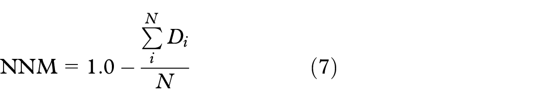
The NNM quantifies the distance preservation using the similarity of each instance in the whole data with its nearest neighbor in the sampled data. The NNM is given by equation (7), where D i is the smallest distance among the i th instance in the complete data set and the instances in the sample, and N denotes the number of instances. In the original article, the authors normalized each dimension of the data to the range [ 0 , 1 ] . However, this results in the loss of the magnitude of the dimensions, hampering our feature weighting process. Therefore, we change the normalization per dimension by a unit vector normalization per instance to avoid such an effect. The output of NNM is within the interval [ 0 , 1 ] with larger values indicating better results

NNM = 1 . 0 − ∑ i N D i N

(7)

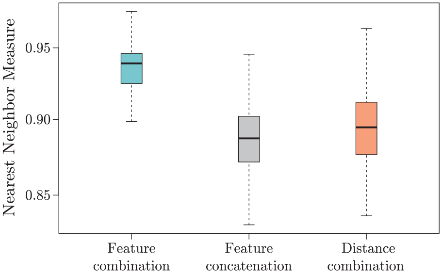
We compare the NNM values of our feature fusion with two baselines: feature concatenation and distance fusion (see section “Related Work”). Boxplots in Figure 7 show that our approach outperforms the other two baselines by at least 5 % . The mean value of our method is 0 . 9365 , and the baselines achieved are 0 . 8877 and 0 . 8958 , respectively. Hence, our method preserves more accurately the data patterns presented in the sample and its distribution in the whole data set fusion.

OPEN IN VIEWER

Figure 7.

The NNM evaluation. We compare our approach of user-guided feature fusion (light green box), with two baselines: feature concatenation, and feature distance combination. Our feature fusion strategy surpasses current state-of-the-art strategies, indicating that the similarity patterns observed in the sample data combination are preserved in the complete data set fusion.

Qualitative evaluation

Besides the quantitative evaluation, we also present an example based on projections for qualitative evaluation. The reasoning is to project the complete combined data set ( V ¯ ) , showing that the patterns observed in the sample projection ( U ¯ ) are preserved on the complete projection. In this example, we use our approach to explore large photo collections considering different user perspectives about similarity among images. We use the photographers data set. In addition to the features described in subsection “Features”, we create a new set of features to describe each photographer. We use Wikipedia articles about each photographer and construct a bag-of-words vector to represent them. Photos of the same photographer share the same feature vector, and the similarity among photos is defined as the similarity between texts describing the photographers.

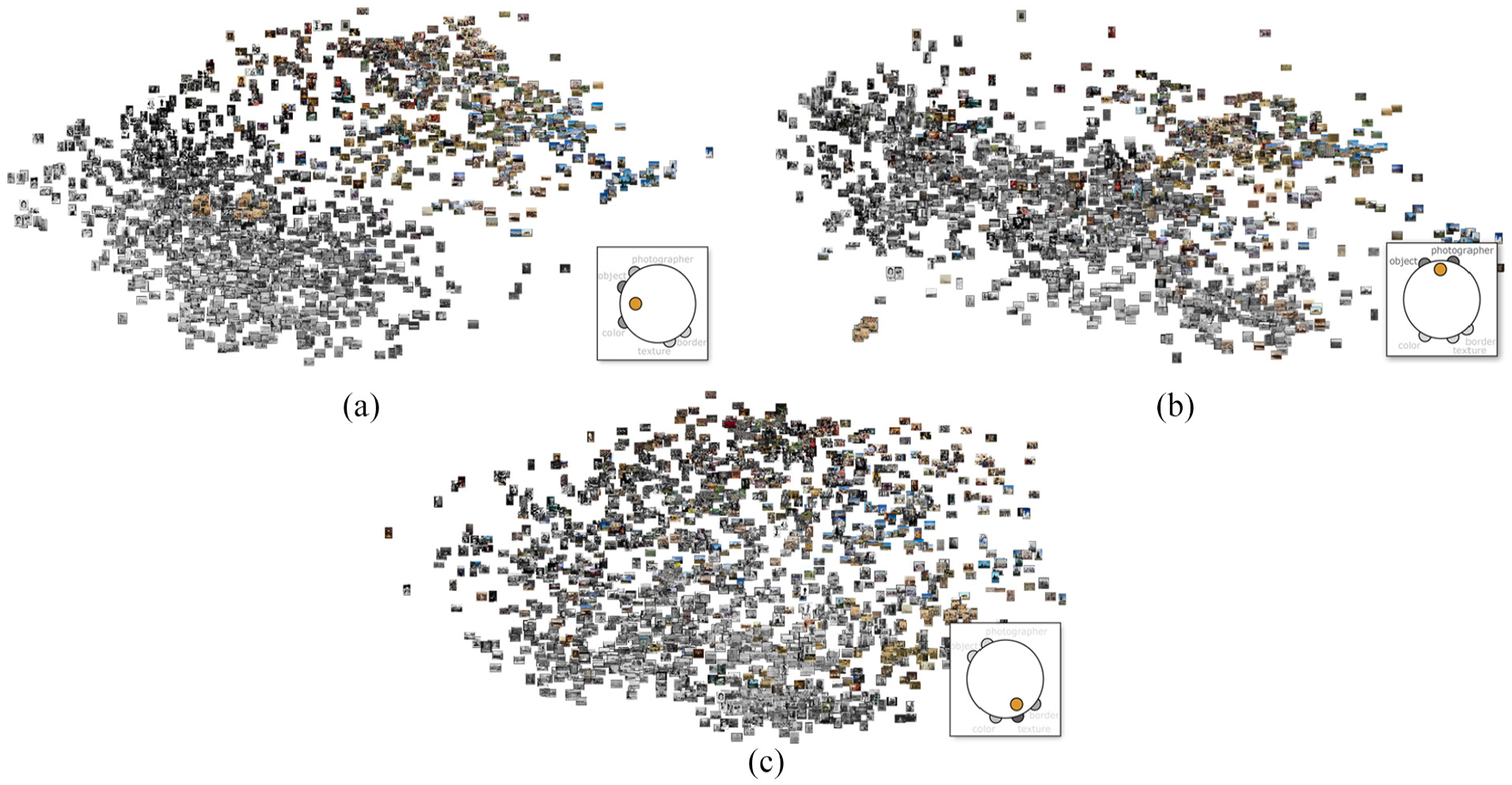
As explained before, based on a sample and using our approach, users can combine different features by employing the combination widget (see Figure 2) until the sample visualization reflects a particular understanding regarding the similarity among photos. Figure 8 shows three different combinations. The first (Figure 8(a)) provides more importance to color and the objects contained in the photos, with little importance given to information about photographers. The second (Figure 8(b)) is defined using the idea of photographic style from ⁴³ fusing objects and Wikipedia features. Finally, the third (Figure 8(c)) shows the result of combining texture, borders and a small amount of color.

OPEN IN VIEWER

Figure 8.

User-defined similarity configurations. Based on a small sample, users can interactively combine different features seeking for the combination that best approaches a particular point of view. This combination is then propagated to the entire data set for a complete projection. The widget at the bottom-right helps to control such combination and indicates the importance of each feature. (a) The combination provides more importance to color and the objects contained in the photos. (b) It gives more importance to the objects and the information about the photographers and (c) It provides more importance to texture, border, and color features.

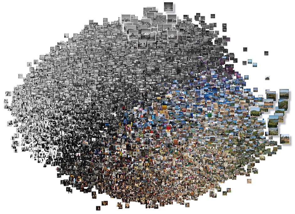
Once a feature combination has been defined that reflects the users’ point of view, a projection representing the complete photo collection is constructed. Figure 9 shows the produced layout using the weights established in Figure 8(a). In this figure, since the color is an important feature, we observe a clear separation between black-and-white and colorful images. Also, given the weight assigned to the feature representing objects, it is possible to notice a separation among photos of people, landscapes, and houses in certain regions of the figure. We zoom in on two small portions of the projection (at the top and at the right side) to show this effect. On the colored images (right), we observe images with sky and forest. On the gray images (top), we observe houses, sky, and forest.

OPEN IN VIEWER

Figure 9.

Photographers data set projection using the weight combination of Figure 8 (a). Since a larger weight is assigned to the color feature, a clear global separation between black-and-white and colorful photos can be observed. This configuration also considers the presence of objects and photographer information.

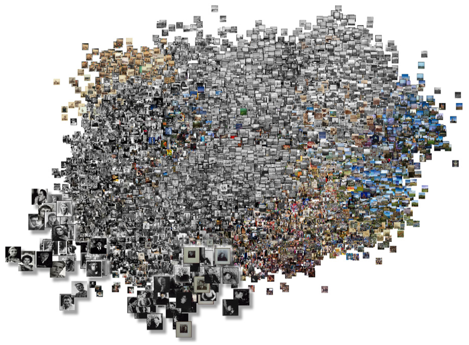
Figure 10 depicts the final projection using the weights defined in Figure 8(b). In this figure, we zoom in on a region at the bottom-left, and here, we mainly find portrait images. Remember that in this weight combination, our goal was to represent the photographic style. The selected photos are from two well-known photographers, Van Vechten and Curtis, who mostly work with portraits, presenting similar styles. ⁴³ These examples qualitatively attest that the similarity patterns observed on the sample projection are preserved in the complete projection, corroborating the quantitative results measured using the NNM index.

OPEN IN VIEWER

Figure 10.

Photographers data set projection using the weight combination of Figure 8 (b). A larger weight is assigned to the object and photographers features. Photos with similar visual features are grouped. The zoom-in region (bottom-left) shows photos of well-known photographers that share similar styles (portrait photos).

Application: user-guided clustering

One of the most appealing application scenarios for our approach is to assist non-supervised data mining strategies, such as clustering techniques. Clustering techniques seek to split sets of data instances into groups so that instances belonging to the same group are more similar to each other than to those in other groups. Typically, clustering is a subjective task that depends on the way the similarity is computed, which could vary from user to user, and the ability to explicitly control and understand similarity is the benefit our approach offers.

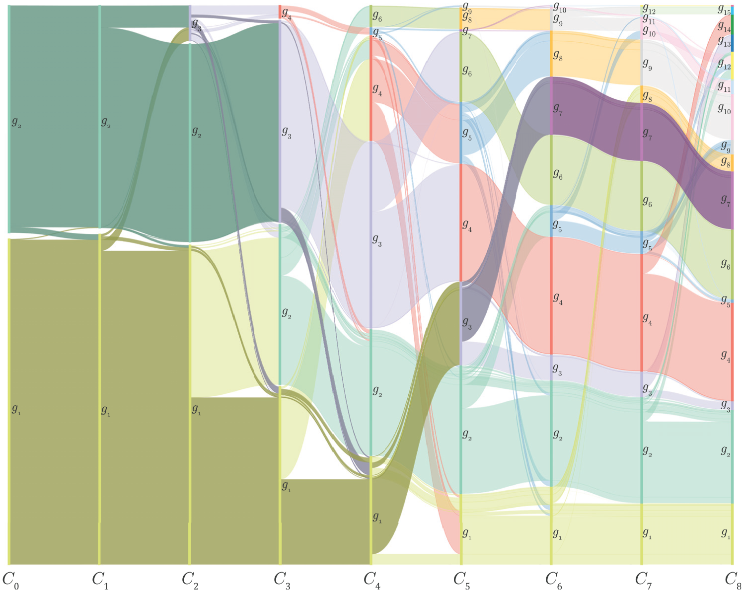
Following, we present an example of using our approach to control clustering results of a sample from the photographers data set containing 7800 instances. In this example, we define different weights for features and observe how this influences the composed groups. In Figure 11, we analyze the transition between color and Wikipedia features. Color starts with weight 1 and decreases to weight 0 as Wikipedia weight increases from 0 to 1 . We generate new fused features in each intermediate state. In each combination state, we compute clusters using the mean shift algorithm. ⁴⁷ We opt to use this algorithm because we do not need to provide the number of clusters as input, so the produced results directly reflect the provided similarity (or combination of features).

OPEN IN VIEWER

Figure 11.

Using parallel sets to visualize cluster formation. The parallel sets visualization shows nine clusterings results computed using the means shift algorithm. Axes C 0 and C 8 represent the clustering results for color and Wikipedia features, respectively. Intermediate clusterings denote combinations of these features.

We display the different clustering configurations (for each combination) using the parallel sets. ⁴⁸ In the parallel sets, the vertical axes represent different clusterings C k , where k indicates a different weight combination of features. All axes contain a set of groups where different colors represent different groups. Curves between axis k and k + 1 are colored using the colors of the groups in C k . This coloring scheme improves the perception of membership changes between different clusterings results. To reduce cluttering, we implement a simple filtering strategy to remove non-relevant curves. For each group in C k , we evaluate how many instances from this group are redistributed in the groups in C k + 1 . If the quantity is less than a percentage threshold, the curves representing these instances are removed. This threshold is a user parameter and can be adjusted accordingly.

Figure 11 shows parallel sets with 9 axes representing clusterings results ( C 0 , C 1 , . . . , C 8 ) with a filtering threshold equal to 0.1. C 0 axis represents the results for the color feature only (no Wikipedia feature is considered). It has two groups, one presenting colorful photos and the other black-and-white photos. C 1 shows fused features with 0 . 79 weight to color and 0 . 21 weight to Wikipedia. Most of the two groups presented in C 0 remain in C 1 , but some instances change their membership.

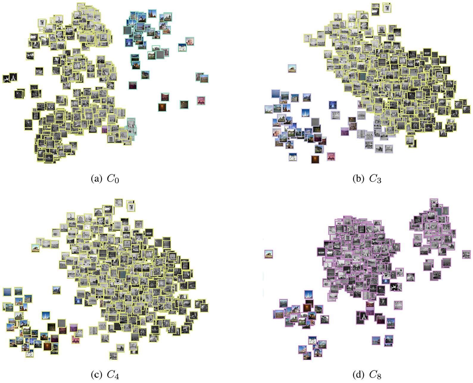
From C 4 , more groups are composed, and the colorful and black-and-white photo division is lost. Finally, C 8 represents the clustering for the Wikipedia feature only (no color feature). Note that from clusterings C 6 to C 8 , the groups are more stable, that is, most of the items in a particular group tend to be assigned to the same group as k increases. In order to analyze the semantic meaning of the groups, we select the purple group ( g 7 ) from C 8 , and we check its correspondent instances backward. Photos of that group were taken by Brumfield, Gottscho, and Horydczak, which are three iconic American photographers. We map the data from C 8 ( g 7 ) to the visual space using the force-scheme technique. ⁴⁹ Figure 12(d) shows the result where each photo border is colored with its group color. As can be observed, photos are similar in content and appearance, as the work of their photographers is focused on architectural photography. We also observe that there is a mixture of colorful and black-and-white photos in this group. However, clustering C 0 shows a clear separation between these two types of photos (Figure 12(a)). Looking at the sequence of curves from clustering C 8 to C 0 , it is possible to analyze the g 7 group and see when photos of this group are merged backward. We highlighted the path in the parallel set with darker colors for easy navigation. From C 8 to C 4 , the groups are stable. Instances of these groups are also projected and depicted in Figure 12(d) and (c). In C 4 , g 1 is formed with instances from C 3 ( g 1 ) and C 3 ( g 3 ) groups. Corresponding instances from C 3 are mapped in Figure 12(b). Note that in C 3 , colorful and black-and-white photos are mixed.

OPEN IN VIEWER

Figure 12.

Projections produced by the force-scheme technique for the purple group ( g 7 ) of instances in C 8 . The color of the border indicates the group the photo belongs to. The purple group instances are selected from C 0 , C 3 , and C 4 and mapped in (a), (b), and (c), respectively. The projection of the purple group in C 8 is shown in (d). In (a), two groups are visible. In (b), these groups are less separate. Both in (c) and (d), there is only one group according to the clustering technique. However, in (d) there is a small group inside this group that distinguishes three photographers with similar styles.

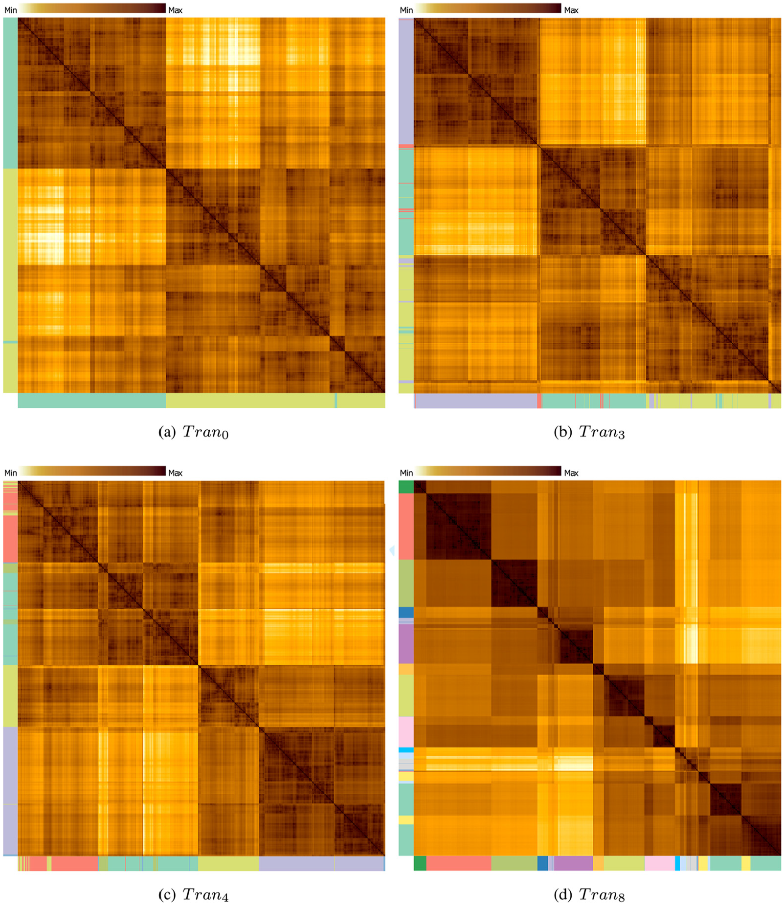
Parallel sets are useful tools to show the difference between clustering results. However, they do not show the similarity relationships between instances. In order to explore clusters and the relationships between instances, we also visualize the pairwise dissimilarity matrix produced from a given feature combination as a heatmap. In our representation, similar items are rendered in brown colors, whereas dissimilar ones are rendered in pale orange colors. The order (rows and columns) of our representation is obtained using the position of the leaves in a dendrogram generated by average linkage hierarchical clustering.^50–52

Figure 13 shows dissimilarity matrices using the same weight combinations that generate C 0 , C 3 , C 4 , and C 8 on parallel sets. In Figure 13(a), we can spot two groups (two dominant brown areas on the main diagonal). The colored margins indicate the groups of the instances given by the clustering algorithm. In Figure 13(b), the two major groups remain, but sub-groups can be noticed inside the larger ones. Figure 13(c) also shows two significant brown areas on the diagonal. However, these groups have the same size. In the previous matrices, one group is bigger than the other because the color feature has more weight and the data set has more black-and-white than colorful photos. In Figure 13(c), the Wikipedia feature begins to have more contribution in the combination process forming clusters that group photos according to style and color. Finally, in Figure 13(d), there are several groups on the main diagonal and two major groups that intersect. A possible explanation is that some photographers tend to shoot similar object categories, but they are from different schools of thought. ⁴³

OPEN IN VIEWER

Figure 13.

Similarity matrix for four different weight combinations. (a) represents color feature only, showing two groups (brown areas on the main diagonal). (b) and (c) represent different weights for color, and Wikipedia features, both displaying two major brown areas but with different sizes. (d) represents the Wikipedia feature only, and it has several small groups on the diagonal and two major intersected groups. These visualizations show how the different weight combinations influence the similarity calculation between instances, matching with the group formation presented by the parallel sets.

Discussion and limitations

The quantitative and qualitative results presented in section “Results and Evaluation” show that the patterns observed on the sample feature fusion ( U ¯ ) are accurately represented in the final feature fusion ( V ¯ ) , suggesting that similarity relationships can be successfully controlled through the manipulation of small portions of large data sets. However, as in any sampling process, we are susceptive to misrepresentations of patterns that could reduce the quality of the final result. We tried to address this using a clustering technique to sample the data from different features and merging these samples. Nevertheless, it is not possible to guarantee that misrepresentation will not occur. This is the price of supporting a real-time approach, and real-time is a critical element in an exploratory process that is based on user judgments to define the “correct” answer—the right combination of features that reflect a personal point of view about similarity. In this scenario, the ability to allow users to perform and check different feature combinations instantaneously is of vital importance. Moreover, allowing users to interact with small samples reduces the cognitive overload imposed on them, especially when handling large data sets.

A critical aspect of our approach is that the resulting feature fusion is an m -dimensional data set, so not intended for visualization purposes (although it can be visualized as any multidimensional data set). Thereby, the user involvement in our process is through the feature combination widget and the analysis of the weight combination via the sample visualization (first phase of our approach). Although we have presented visual representations for the clustering results, they are meant only to show how effectively the feature combination can be used to control the clustering results. Our intention was not to provide a new visualization for clustering methods. Moreover, the interaction is not with the clustering parameters but through the manipulation of the input space, so our approach could be employed with other subjective unsupervised techniques that rely on user expectations.

Finally, our approach provides support to unsupervised tasks where the result is subject to individual perception, like on the definition of similarity among images, instead of proposing a mechanism to improve a quality measure, like accuracy for classification. For enhancing quality measures, especially for supervised classification, user interaction usually is not necessary, and deep learning approaches tend to produce unbeatable results, particularly when processing image collections. However, for subjective unsupervised methods, where user expectations and interpretability are essential components to control the final results and to understand them (based on the feature meaning), is of utmost importance, and this is the core contribution of our approach.

Conclusion

In this article, we proposed a novel approach for feature fusion that successfully allows users to control the fusion process. It is a two-step strategy where, starting from a small sample of the input data, users can quickly test different feature combinations and check in real-time the resulting similarity relationships. Once a combination that matches the user expectation is defined, it is propagated to the whole data set through an affine transformation. Our experiments show that the complete data set combination preserves the similarities from the sample configuration, making our approach a very flexible mechanism to assist the feature fusion process.

We have applied the proposed feature fusion approach to allow users to control and understand the results of clustering techniques. Clustering is one of the most attractive application scenarios for our approach given the subjectiveness involved in unsupervised tasks. Currently, visualization assisted clustering techniques only allow users to control the results by changing technique parameters.^53–56 Enabling users to guide the input feature configuration renders a much more flexible control, since users can explicitly steer the semantics of the input data and the similarity relationships (e.g. images are similar due to the color vs images are similar due to the presence of objects). Therefore, the proposed methodology controls the cluster formation while still allowing for a natural interpretation of the composed groups.