Stable visualization of connected components in dynamic graphs

Abstract

One of the primary goals of many systems for the visual analysis of dynamically changing networks is to maintain the stability of the drawing throughout the sequence of graph changes. We investigate the scenario where the changes are determined by a stream of events, each being either an edge addition or an edge removal. The visualization must be updated immediately after each new event is received. Our main goal is to provide the user with an intuitive visualization that highlights the different connected components of the graph while preserving the user’s mental map after each event. The drawing stability is measured in terms of changes in the orthogonal relationships between vertices of two consecutive drawings. We describe two different visualization models, one for the 1-dimensional space and the other for the 2-dimensional space. In both models the connected components are drawn inside rectangular regions. To validate our approach, we report the results of an experimental analysis that compares the drawing stability of the online algorithm with that of an offline algorithm that knows in advance the whole sequence of events. We also present a case study of our online algorithm on a collaboration network.

Keywords

Dynamic graph visualization drawing stability clustering visualization connected components arc diagrams orthogonal drawings

Introduction

Dynamic networks occur in many application domains, including sociology, finance, biology, cybersecurity, and telecommunications.¹ For example, in a social network the edges can change depending on the evolution of the relationships between the different subjects. In a biological network that describes the interaction between genes and proteins, the edges can change depending on the temporal evolution of gene expression levels. In a computer network, the vertices represent different machines and communication links between the different vertices may become unavailable or may be resumed over time, depending on temporary hardware or software failures. All these application domains can strongly benefit from the use of visualization to support the analysis of how the phenomena modeled by the networks change over time.²

One of the primary goals of many systems for the visual analysis of dynamic networks is to maximize the drawing stability throughout the sequence of graph changes, which is correlated with the preservation of the user’s mental map.^2,3 Many user experiments have been conducted to assess the importance of keeping a graph layout stable with respect to the execution of different analysis tasks. An early study by Purchase et al.⁴ focuses on hierarchical graph layouts and confirms this assumption only for some types of tasks. Archambault et al.⁵ experimentally study the benefit of preserving the mental map under two different ways of showing graph evolutions, namely animation and presentation of small multiples; they found that in both cases preserving the mental map seems to have little influence in terms of error rate and response time. Qualitative data collected by Archambault and Purchase⁶ suggest that, in terms of the users perception, preserving the mental map makes memorability tasks easier, although no statistic evidence is found on the user performances. Memorability tasks are important for information discovery and they are related to the capability of a user to remember elements and changes in the evolving network. Archambault and Purchase⁷ summarize the rich set of experimental works aimed to assess the impact of mental map preservation. Although they remark that none of these works has found conclusive evidence that supports the effectiveness of the mental map in the comprehension of a dynamic graph series, they also highlight possible limits of previous experiments and provide new insights for further investigations. Also, based on some experiments on static graphs, they conjecture that revisitation tasks on dynamic graphs could benefit from keeping the drawing stable. Revisitation tasks require to remember where objects in a particular space are located and how they can be reached a second time. A recent user study by Federico and Miksch⁸ investigates the role of an interaction technique for layout stability adjustment and gives some evidence that this type of interaction may increase accuracy in the execution of specific analysis tasks. Another recent study by Lezama et al.⁹ tries to further investigate the trade-off between drawing stability and drawing readability, based on a new mathematical model.

In this paper we restrict our attention to evolving networks where only the set of edges changes over time (while the set of vertices remains stable). Consider, for example, social networks in which the vertices represent a target set of email users and the edges represent their mail exchanges in a desired time window. Or graphs that model the traffic evolution on a LAN and that show only those links whose communication load trespasses a given threshold. More specifically, we study the scenario in which we are given a network with a fixed set of vertices and whose relationships may change over time. We assume that the changes in the network are determined by a stream of events, each being either an edge addition or an edge removal. The visualization must be updated immediately after each new event is received. Our main goal is to design an online algorithm to visually support a network analyst in identifying the different connected components of the graph while easily following the graph changes. In this respect, we believe that drastic changes in the graph layout should be avoided when small changes in the graph topology happen. In particular, any user would be totally disoriented if, after the addition or the removal of a single edge in the network, many vertices change their relative positions.

Contribution

We describe two different visualization models and related online algorithms, one for the 1-dimensional space and the other for the 2-dimensional space. The 1-dimensional visualization model adopts an arc diagram style,¹⁰ while the 2-dimensional model exploits a variant of orthogonal drawings,^11,12 that is, drawings whose vertices are mapped to points of an integer grid and edges are drawn as chains of horizontal and vertical segments. In both models the connected components are regarded as clusters and are drawn inside rectangular regions. The drawing stability is measured in terms of changes in the orthogonal relationships of the vertices between two consecutive drawings, as suggested in a seminal paper by Misue et al.³ As a byproduct, our approach also satisfies a larger set of stability requirements that were proposed by Frishman and Tal¹³ about dynamic visualization of clustered graphs. In fact, our algorithmic strategy can also be adopted in the more general scenario in which the clusters do not necessarily represent connected components, and they can be merged or split.

To validate the proposed approach, we experimentally show that our online algorithm is competitive with an offline strategy that knows the whole sequence of events and that maximizes the drawing stability over all this sequence. We also present a case study of our online algorithm on a collaboration network.

Related work

The research in this work fits in the broad area of dynamic graph visualization. According to a recent survey of Beck et al.,² the rich literature in this area can be classified into two main categories, timeline approaches and animation approaches, based on how changes in the graph are conveyed to the user.

Timeline approaches use a time-to-space mapping that creates static visualizations in which the time dimension is embedded into the graph layouts. Examples include juxtaposed or superimposed node-link diagrams, where the time dimension coincides with a geometric axis that is visually separated by the graph layouts.^14–16 Another example are integrated diagrams in which the timeline is woven into the graph layout.^17,18 A static visualization for dynamic trees, based on the popular treemap convention is proposed by Köpp and Weinkauf.¹⁹

Animation approaches adopt a time-to-time mapping that creates a sequence of distinct graph layouts, one for each time step, and shows to the user a layout per time. Examples of these approaches are presented both for online scenarios, where only past data can be used to compute the visualization in each time step,^3,21,22 and for offline scenarios, where future temporal changes are also known, and the layout algorithm can take advantage of this knowledge to improve drawing stability throughout the animation.^23–25 Our work belongs to the class of online animation approaches, since we promptly update the graph layout at each event of a temporal stream of changes. We also compare the drawing stability cost of our strategy with an offline strategy that knows the entire sequence of events in advance.

Our research is also strongly related to the problem of dynamic drawing of clustered graphs with only one level of clusters, where a cluster of vertices is drawn inside a rectangular region. Frishman and Tal¹³ address this problem and indicate a set of requirements in terms of vertex and cluster stability that the drawing algorithm should pursue. They describe a force-directed drawing algorithm with straight-line edges that takes as input a sequence of clustered graphs and that heuristically attempts to match the given requirements as much as possible. In our framework, clusters are not given as part of the input; they coincide with the connected components of the graph and therefore they are automatically induced by the changes in the set of edges. Also, we use neither straight-line edges nor a force-directed strategy; instead, we adopt drawing models and algorithms that make it possible to minimize (in an exact way) the drawing stability cost at each new event in linear time (refer to the next section). Alternative visualization approaches for dynamic drawing of clustered graphs have also been studied, where clusters are possibly organized into a hierarchy, graphs are not necessarily represented as node-link diagrams, and clusters are not necessarily represented as rectangular regions; we refer the reader to the following surveys or recent papers on the topic.^2,26,27

Finally, our work is clearly related to the design of algorithmic techniques to draw graphs with multiple connected components. Several algorithms have been proposed in the literature to compute compact layouts of such graphs.^28–31 These algorithms assume that the graph is static and aim to arrange the different components in such a way that the area of the drawing is minimized and two components do not overlap. Gansner et al.³² consider a dynamic scenario in which an initial drawing configuration for the different connected components of a graph is given, and each connected component may grow up and cause overlaps with other components. For this scenario, they propose a new drawing approach that removes overlaps between components and that keeps the relative positions of the different components stable. Their approach modifies and combines node-overlap removal techniques³³ and polyomino-based packing techniques.²⁹ Differently from our scenario, their approach is aimed to support a map metaphor visualization for clustered graphs with straight-line edges.

Models, metrics, and algorithms

In our dynamic scenario we start from an initial graph $G_{0}$ ; a subsequent stream of temporal events may change the set of edges of $G_{0}$ , while the set of vertices of $G_{0}$ remains unchanged. We formalize this scenario as follows. Consider a temporal sequence of graphs $G_{0}, G_{1}, \dots, G_{k}$ such that for each $i = 0, \dots, k$ , $G_{i} = (V, E_{i})$ is the graph at time $t_{i}$ and, for each $0 \leq i \leq k - 1$ , the set $E_{i + 1}$ is obtained from $E_{i}$ by either adding a single edge or removing a single edge. Denote by $C_{i}$ the set of connected components of the graph $G_{i}$ . The addition of an edge to $G_{i}$ may cause the merging of two connected components into a single one, in which case $| C_{i + 1} | = | C_{i} | - 1$ . The deletion of a single edge to $G_{i}$ may cause the splitting of a connected component into two distinct components, in which case $| C_{i + 1} | = | C_{i} | + 1$ .

We want to visually represent each graph $G_{i}$ by means of a node-link diagram $Γ_{i}$ in the plane such that the different connected components are clearly distinguishable. To this aim, we require that all the vertices of each connected component $c \in C_{i}$ are inside a rectangular region $R (c)$ and for any two components $c, c' \in C_{i}$ , $R (c) \cap R (c') = \emptyset$ and no edge of $c$ intersects $R (c')$ . Within these constraints, we consider two specific drawing models, one that places the vertices in the 1-dimensional space (1D drawing model) and the other that places the vertices in the 2-dimensional space (2D drawing model). For each of these models, we design an online drawing algorithm that aims to maximize the drawing stability when it computes $Γ_{i + 1}$ from $Γ_{i}$ . We measure the drawing stability in terms of changes in the orthogonal ordering between pair of vertices.³ As it will be clear in the next section, thanks to our drawing models, this stability criterion also guarantees the following stability criteria indicated by Frishman and Tal¹³ for dynamic drawing of clustered graphs, where our clusters coincide with the connected components of the graph: (1) The movement of clusters between successive drawings should be small; clusters that are not modified should remain in their previous (relative) position if possible; (2) the change in the size of clusters between successive drawings should be minimal, when the number of vertices in the cluster is similar; (3) movement of vertices inside a cluster should be minimized; (4) the size of each cluster should be proportional to the number of vertices it contains; (5) the drawing of each cluster should be compact; and (6) overlapping between vertices should be avoided and overlapping between cluster boundaries should be minimal.

Formally, for a vertex $v \in V$ , denote by $(x_{v}^{i}, y_{v}^{i})$ the position of $v$ in $Γ_{i}$ and by $(x_{v}^{i + 1}, y_{v}^{i + 1})$ the position of $v$ in $Γ_{i + 1}$ . For any two distinct vertices $u, w \in V$ , the orthogonal ordering of $u$ and $v$ is preserved while passing from $Γ_{i}$ to $Γ_{i + 1}$ if the following relations hold:

(a) $x_{u}^{i + 1} < x_{w}^{i + 1} \Leftrightarrow x_{u}^{i} < x_{w}^{i}$

(b) $x_{u}^{i + 1} = x_{w}^{i + 1} \Leftrightarrow x_{u}^{i} = x_{w}^{i}$

(d) $y_{u}^{i + 1} = y_{w}^{i + 1} \Leftrightarrow y_{u}^{i} = y_{w}^{i}$

Hence, to measure the changes in the orthogonal ordering of a pair of vertices $u$ and $w$ in two consecutive drawings $Γ_{i}$ and $Γ_{i + 1}$ , we define a cost function $h_{i, i + 1} (u, w)$ whose value is the number of relations (a)–(d) that are false, that is, that do not hold. The drawing stability cost for a pair of consecutive drawings $Γ_{i}$ and $Γ_{i + 1}$ is defined as the sum of the aforementioned cost function over all pairs of vertices, that is:

H (Γ_{i}, Γ_{i + 1}) = \sum_{u, w \in V} h_{i, i + 1} (u, w) .

Maximizing the drawing stability on two consecutive drawings $Γ_{i}$ and $Γ_{i + 1}$ equals to minimizing the drawing stability cost $H (Γ_{i}, Γ_{i + 1})$ .

The drawing stability cost of the whole sequence of drawings $Γ_{0}, Γ_{1}, \dots, Γ_{k}$ can be measured in different ways. In the implementation and experimental section, we will consider the total stability cost, defined as $\sum_{i = 0}^{k - 1} H (Γ_{i}, Γ_{i + 1})$ , and the maximum stability cost, defined as ${max}_{i = 0}^{k - 1} H (Γ_{i}, Γ_{i + 1})$ .

We remark that, in the context of orthogonal drawings, different measures of mental map preservation have been proposed by Bridgeman and Tamassia.³⁴ Not all their measures apply to our scenario, because they are defined to quantify the difference between two drawings of the same graph rather than between consecutive drawings of a dynamic graph. However, minimizing our drawing stability metric for the 2D visualization model (which exploits a restriction of the orthogonal drawing convention) implies the optimization of some of the measures in Bridgeman and Tamassia,³⁴ namely the orthogonal ordering measure and the Euclidean distance measure. In the following subsections we describe our 1D and 2D drawing models and the related online drawing algorithms. For a connected component $c \in C_{i}$ , we denote by $n (c)$ and $m (c)$ the number of vertices and the number of edges of $c$ , respectively.

1D drawing model

Our drawing model that places the vertices in 1D is inspired by the popular arc diagram style, where the vertices of the graph lie on a common horizontal line, which we call spine, and the edges are drawn as semicircles above or below the spine. Although the name “arc diagram” stems from a work on the visualization of repetition patterns in string,¹⁰ this drawing style has a much older tradition and has been originally used to study crossing numbers of graphs.^35,36 Arc diagrams are sometimes called line embeddings,³⁷ and they are also referred to as two-page book embeddings if they have no edge crossings.³⁸ Several papers also study edge crossings and crossing minimization in arc-diagrams.³⁹⁻⁴³ Applications of arc diagrams to the visualization of directed graphs have also been proposed.⁴⁴ We finally remark that arc diagrams are conceptually related to circular drawings and chord diagrams, where the vertices are placed on a circle and the edges are lines that can be embedded inside or outside this circle.^45–47 Chord diagrams have been recently proposed for the visual analysis of dynamic graphs in distributed software profiling.⁴⁸ From a dynamic graph drawing perspective, minimizing the changes in the linear ordering of our 1D drawing model seems to be related to the problem of minimizing crossings in a storyline visualization.^49,50 Indeed, a crossing between the lines representing two characters in a storyline visualization occurs when we invert the linear ordering of these lines along the vertical axis.

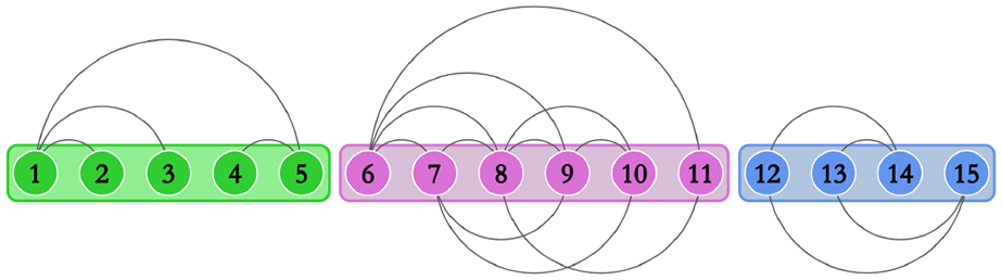
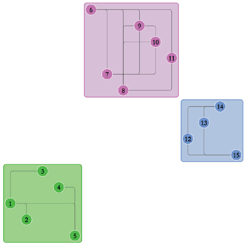
We compute the drawing $Γ_{i}$ of $G_{i}$ as an arc diagram where all vertices are equispaced and for each edge $(u, v) \in E_{i}$ the diameter of its corresponding semicircle equals the Euclidean distance between $u$ and $v$ . Also, the fact that all the vertices of a connected component of $G_{i}$ are inside a rectangular region implies that these vertices are all consecutive in the linear ordering along the spine. We call such a drawing a connected-component-arc diagram or a cc-arc diagram for short. An example is shown in Figure 1.

Figure 1.

A cc-arc-diagram of a graph with 15 vertices and 3 connected components; the rectangular regions of the different connected components have different colors.

Clearly, in a cc-arc diagram all vertices have the same $y$ -coordinate and no two vertices have the same $x$ -coordinate. Thus, changes in the orthogonal ordering of the vertices imply that relation (a) is violated, that is, the $x$ -ordering of some pairs of vertices is modified. The drawing stability cost $H (Γ_{i}, Γ_{i + 1})$ equals the number of pairs of vertices that change their $x$ -ordering in $Γ_{i}$ and $Γ_{i + 1}$ .

Our online drawing algorithm for dynamic cc-arc diagrams computes $Γ_{i + 1}$ from $Γ_{i}$ , depending on the type of event at time $t_{i + 1}$ .

Edge addition. When $G_{i + 1}$ is obtained from $G_{i}$ by adding a new edge $e = (u, v)$ , two cases are possible:

$u$ and $v$ belong to the same component $c \in C_{i}$ . In this case, $| C_{i + 1} | = | C_{i} |$ and $e$ can be trivially drawn without any change in the orthogonal ordering of the vertices, that is, $H (Γ_{i}, Γ_{i + 1}) = 0$ . Note that, for what concerns the drawing stability, $e$ can be arbitrarily drawn above or below the spine; in this case the edge addition is executed in $O (1)$ time. Otherwise, one can choose the option that optimizes some desired quality metrics; for example, one can make the choice that minimizes the number of edge crossings, which takes $O (m (c))$ time.

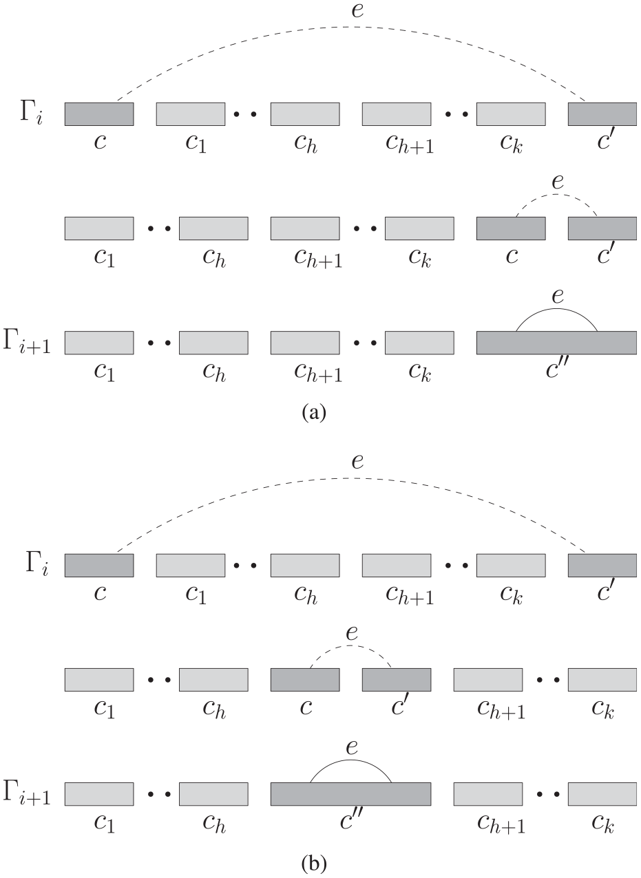
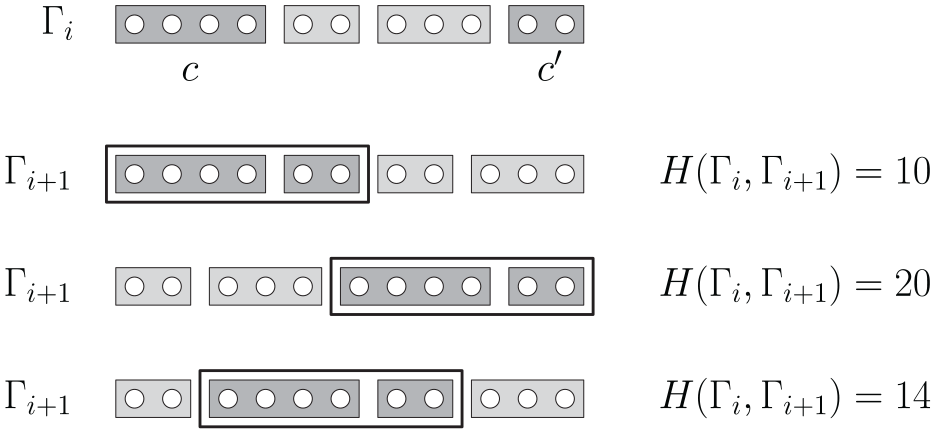
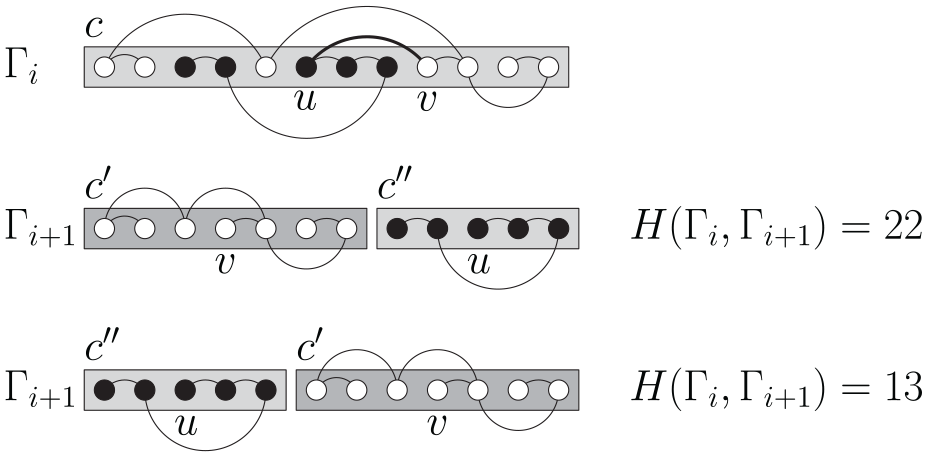
$u$ and $v$ belong to two distinct components $c \in C_{i}$ and $c' \in C_{i}$ , respectively. In this case, the two components $c$ and $c'$ are merged into a single component $c ″ \in C_{i + 1}$ , which also includes edge $e$ . Let $c_{1}, \dots, c_{k}$ be the left-to-right sequence of connected components of $G_{i}$ between $c$ and $c'$ (refer to Figure 2 for a schematic illustration). Merging $c$ and $c'$ into $c ″$ requires to make $c$ and $c'$ consecutive along the spine. This can be done in several ways. A possibility is to translate the vertices of $c$ toward $c'$ , so that $c ″$ immediately follows $c_{k}$ in $Γ_{i + 1}$ (see Figure 2(a)). A symmetric choice is to translate the vertices of $c'$ toward $c$ , so that $c ″$ immediately precedes $c_{1}$ in $Γ_{i + 1}$ . Another choice is to translate $c$ to the right and $c'$ to the left, so that $c ″$ will be between two components $c_{h}$ and $c_{h + 1}$ in $Γ_{i + 1}$ , for some $h \in {1, \dots, k}$ (see Figure 2(b)). Our algorithm places $c ″$ immediately after $c_{k}$ if $n (c) \leq n (c')$ , and immediately before $c_{1}$ otherwise. Lemma 1 shows that this choice minimizes the drawing stability cost $H (Γ_{i}, Γ_{i + 1})$ . This translation takes $O (\sum_{j = 1, \dots, k} n (c_{j}) + min {n (c), n (c')})$ time, needed to update the coordinates of the vertices between $c$ and $c'$ plus the vertices of one among $c$ and $c'$ . Then, edge $e$ is added as in the previous case.

Figure 2.

Different ways of merging two components $c$ and $c'$ into a single component $c ″$ : (a) $c$ is translated toward $c'$ and (b) $c$ and $c'$ are translated one toward the other.

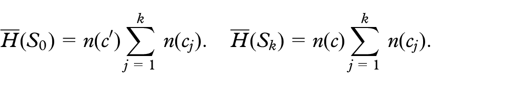
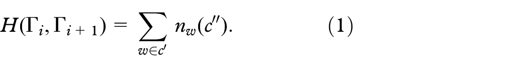
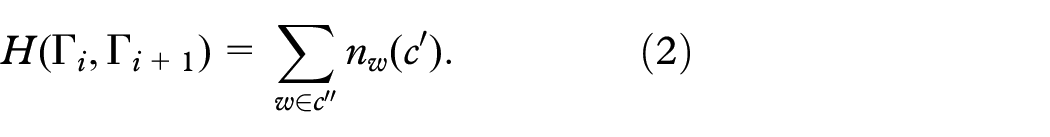
Lemma 1. Let $S = c, c_{1}, \dots, c_{k}, c'$ be a subsequence of connected components along the spine of a cc-arc diagram $Γ_{i}$ and let $c ″$ be the connected component of $Γ_{i + 1}$ obtained by merging $c$ and $c'$ . The cost $H (Γ_{i}, Γ_{i + 1})$ is minimized by replacing $S$ with the new subsequence $c_{1}, \dots, c_{k}, c ″$ if $n (c) \leq n (c')$ , and by the subsequence $c ″, c_{1}, \dots, c_{k}$ otherwise.

Proof. Denote by $S_{0}$ the subsequence $c ″, c_{1}, \dots, c_{k}$ of $Γ_{i + 1}$ , by $S_{k}$ the subsequence $c_{1}, \dots, c_{k}, c ″$ , and by $S_{h}$ the subsequence $c_{1}, \dots, c_{h}, c ″, c_{h + 1}, \dots, c_{k}$ , with $h = 1, \dots, k - 1$ . Denote by $\bar{H} (S_{r})$ the drawing stability cost $H (Γ_{i}, Γ_{i + 1})$ spent to obtain $S_{r}$ $(r = 0, \dots, k)$ . The subsequence $S_{0}$ requires to translate $c'$ to the left until it meets $c$ ; $S_{k}$ requires to translate $c$ to the right until it meets $c'$ ; $S_{h}$ requires to translate $c$ to the right and $c'$ to the left, until they meet in-between $c_{h}$ and $c_{h + 1}$ . Thus we have the following costs for each subsequence, which correspond to the number of pairs of vertices that change their $x$ -ordering when passing from $Γ_{i}$ to $Γ_{i + 1}$ :

\bar{H} (S_{0}) = n (c') \sum_{j = 1}^{k} n (c_{j}) . \bar{H} (S_{k}) = n (c) \sum_{j = 1}^{k} n (c_{j}) .

\bar{H} (S_{h}) = n (c) \sum_{j = 1}^{h} n (c_{j}) + n (c') \sum_{j = h + 1}^{k} n (c_{j}) .

Hence, if $n (c) \leq n (c')$ , we have $\bar{H} (S_{k}) \leq \bar{H} (S_{0})$ and $\bar{H} (S_{h}) \geq n (c) \sum_{j = 1}^{h} n (c_{j}) + n (c) \sum_{j = h + 1}^{k} n (c_{j}) = \bar{H} (S_{k})$ , thus $S_{k}$ is the cheapest solution. Otherwise, $\bar{H} (S_{0}) \leq \bar{H} (S_{k})$ and $\bar{H} (S_{h}) \geq n (c') \sum_{j = 1}^{h} n (c_{j}) + n (c') \sum_{j = h + 1}^{k} n (c_{j}) = \bar{H} (S_{0})$ , thus $S_{0}$ is the cheapest solution {q.e.d.}.

Figure 3 shows an example of merging two components $c$ and $c'$ and three possible solutions to perform this operation. For each solution the corresponding cost is reported. The cheapest solution consists of moving $c'$ toward $c$ .

Figure 3.

Example of merging two components $c$ and $c'$ in a cc-arc diagram (the edges of the diagram are not shown). Three different solutions and their drawing stability costs are shown. Translating $c'$ toward $c$ is the cheapest solution.

Edge removal. When $G_{i + 1}$ is obtained from $G_{i}$ by removing an edge $e = (u, v)$ , two cases are possible:

the connected component of $e$ remains connected after the removal of $e$ . In this case, $| C_{i + 1} | = | C_{i} |$ and $e$ can be trivially deleted without any change in the orthogonal ordering of the vertices, that is, $H (Γ_{i}, Γ_{i + 1}) = 0$ . This takes $O (1)$ time.

the connected component of $e$ is no longer connected after the removal of $e$ . In this case, denoted by $c \in C_{i}$ the connected component of $e$ in $G_{i}$ , it will be disconnected into two connected components $c', c ″ \in C_{i + 1}$ . Call white and black the vertices of $c'$ and those of $c ″$ , respectively. Clearly, if $u$ is white then $v$ is black, and vice versa. In the drawing $Γ_{i}$ , black and white vertices may be in any order in the $x$ -ordering, while in $Γ_{i + 1}$ all the white vertices (resp. black vertices) must be consecutive in the $x$ -ordering, so that they can be enclosed in the rectangular region $R (c')$ (resp. $R (c ″)$ ). To this aim, we have to translate all the black vertices before the white vertices or vice versa, without changing the relative $x$ -ordering of the vertices with the same color. For each vertex $w \in c'$ (i.e. for a white vertex), denote by $n_{w} (c ″)$ the number of vertices of $c ″$ (i.e. black vertices) that are to the left of $w$ in $Γ_{i}$ . Symmetrically, for a vertex $w \in c ″$ (i.e. for a black vertex), let $n_{w} (c')$ be the number of white vertices to the left of $w$ in $Γ_{i}$ . Translating all the white vertices before the black vertices has the following drawing stability cost:

H (Γ_{i}, Γ_{i + 1}) = \sum_{w \in c'} n_{w} (c ″) .

(1)

Translating all the black vertices before the white vertices has the following cost:

H (Γ_{i}, Γ_{i + 1}) = \sum_{w \in c ″} n_{w} (c') .

(2)

The drawing algorithm will chose the cheapest option between (1) and (2). Making this choice and updating the vertex ordering takes $O (n (c))$ time. For example, Figure 4 depicts a connected component $c$ of a cc-arc-diagram $Γ_{i}$ ; in the next drawing $Γ_{i + 1}$ , edge $(u, v)$ is removed and $c$ is split into two components $c'$ and $c ″$ . The two ways of executing this change are shown, along with their corresponding drawing stability costs.

Figure 4.

Example of splitting a component $c$ into two components $c'$ and $c ″$ in a cc-arc diagram. In the example, the splitting is caused by the removal of an edge $(u, v)$ (the thick edge) from a cc-arc-diagram $Γ_{i}$ . The black vertices will be in the same component as $u$ in $Γ_{i + 1}$ while the white vertices will be in the same component as $v$ . Translating all the black vertices before the white ones causes a smaller drawing stability cost.

2D drawing model

Our 2D drawing model adopts the popular orthogonal drawing convention, where vertices are mapped to points of an integer grid and edges are sequences of horizontal and vertical segments^{12,25,51–53} This kind of drawings has been widely studied for the representation of graphs with clusters of vertices drawn as rectangular regions.^54–57 Our cluster regions correspond to the rectangular regions of the different connected components. Furthermore, in our drawing model we require that each row and each column of the grid contains exactly one vertex of the graph; this means that the drawing fits into a $| V | \times | V |$ grid and there is neither two vertices with the same $x$ -coordinate nor two vertices with the same $y$ -coordinate. Drawings with this property have been recently studied by different authors to support dynamic graph visualizations, because they facilitate the insertion of a vertex or of an edge in the drawing while preserving the user’s mental map. They are called rook-drawings when the edges are straight lines^58,59 and L-drawings when the edges have an orthogonal L-shape, that is, when each edge consists of exactly a vertical segment and a horizontal segment.¹¹ Our 2D drawing model will be called cc-L-drawing, because it is an L-drawing with rectangular regions that enclose the different connected components. Note that, since no vertices share the same $x$ -coordinate or the same $y$ -coordinate, an L-shaped edge in the drawing can always be added without intersecting any vertex, except its end-vertices. Also, two edges may partially overlap, but this does not create ambiguities due to the fact that each edge has an L-shape. These properties remain true even if the clusters do not correspond to the connected components of the graph and there are edges that join vertices that belong to different cluster regions. Figure 5 depicts an example of a cc-L-drawing for the same graph shown in Figure 1.

Figure 5.

A cc-L-drawing of the same graph with 15 vertices and 3 connected components shown in Figure 1.

On the negative side, we remark that rook-like drawings are consuming in terms of area requirement, because they do not allow the reuse of rows and columns. This makes our 2D model mainly suitable for the visualization of relatively small sets of target vertices and their relationships.

The vertex coordinates in a cc-L-drawing can be obtained by combining those of two cc-arc-diagrams, one along the $x$ -axis and the other along the $y$ -axis. The $x$ -ordering and $y$ -ordering of the vertices can be determined independently one of the other, provided that all the vertices of the same connected component are consecutive in each of the two orderings. More formally, if $Γ_{i}$ is a cc-L-drawing at time $t_{i}$ , denote by $Γ_{i}^{x}$ any cc-arc-diagram whose vertex ordering corresponds to the $x$ -ordering of the vertices of $Γ_{i}$ and by $Γ_{i}^{y}$ any cc-arc-diagram whose vertex ordering corresponds to the $y$ -ordering of the vertices of $Γ_{i}$ . Since the drawing stability cost $H (Γ_{i}, Γ_{i + 1})$ only depends on the changes in the $x$ - and $y$ -ordering of the vertices (while it is not affected by the edge routing), it is immediate to see that:

H (Γ_{i}, Γ_{i + 1}) = H (Γ_{i}^{x}, Γ_{i + 1}^{x}) + H (Γ_{i}^{y}, Γ_{i + 1}^{y}) .

(2)

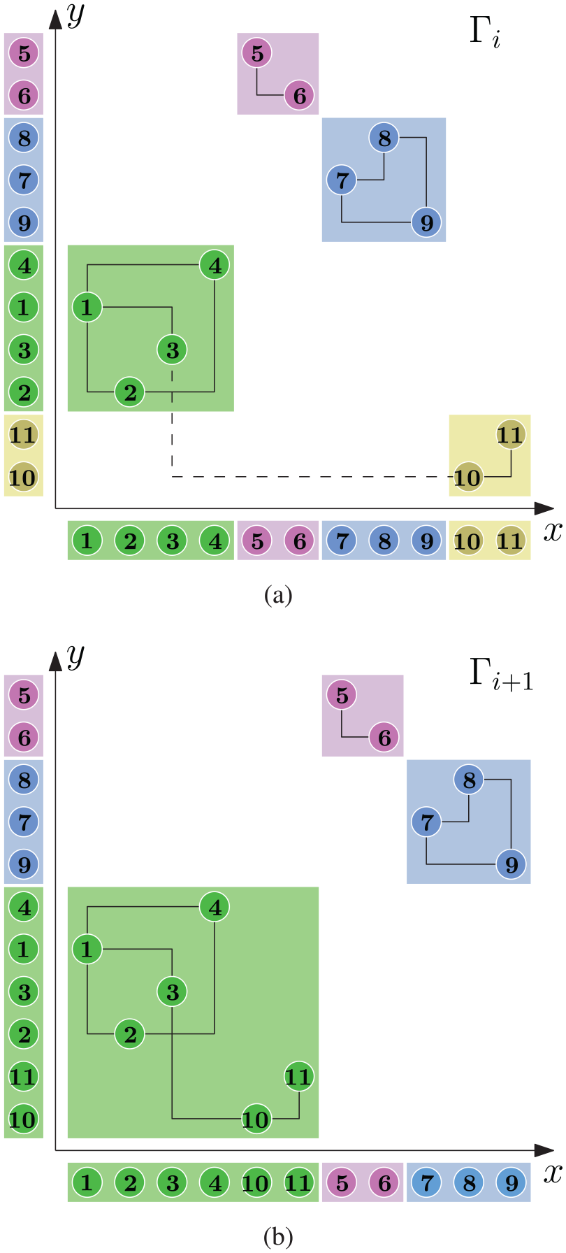
Thanks to this observation, when an edge addition or an edge removal at time $t_{i + 1}$ occurs, our online algorithm for cc-L-drawings can independently apply the same strategies described in the 1D drawing model on $Γ_{i}^{x}$ and on $Γ_{i}^{y}$ in order to compute $Γ_{i + 1}$ . Figure 6 shows an example of edge addition that causes a merge operation; the projections of the vertices along the $x$ -axis and the $y$ -axis are also shown, which represent the linear orderings of the vertices in $Γ_{i}^{x}$ and $Γ_{i}^{y}$ , respectively. Figure 7 shows an example of edge removal that causes a split operation.

Figure 6.

Example of edge addition that causes a merge operation in a cc-L-drawing: (a) a cc-L-drawing $Γ_{i}$ and an edge (dashed) that must be added at time $t_{i + 1}$ and (b) the drawing $Γ_{i + 1}$ obtained by merging the green and the yellow component of $Γ_{i}$ (the resulting component is colored green); the drawing stability cost is minimized by translating the yellow component toward the green component in the $x$ -direction, while the $y$ -ordering of the vertices does not change. Hence, $H (Γ_{i}, Γ_{i + 1}) = 10$ .

Figure 7.

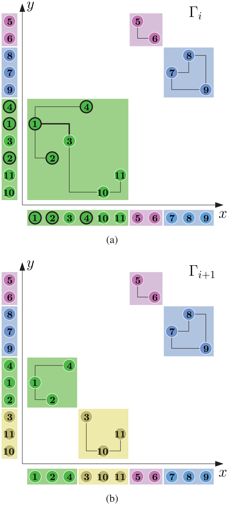
Example of edge removal that causes a split operation in a cc-L-drawing: (a) a cc-L-drawing $Γ_{i}$ with the edge $(1, 3)$ (thicker) that must be removed at time $t_{i + 1}$ ; after the edge removal, the vertices ${1, 2, 4}$ (in bold) will form a component and the vertices ${3, 10, 11}$ will form another component and (b) the drawing $Γ_{i + 1}$ obtained by splitting the green component of $Γ_{i}$ into two components (colored green and yellow, respectively); the drawing stability cost is minimized by moving the bold vertices before the others in each of the two directions. This requires to change the $x$ -ordering of the pair of vertices ${3, 4}$ and the $y$ -ordering of the pair of vertices ${2, 3}$ . Hence, $H (Γ_{i}, Γ_{i + 1}) = 2$ .

Implementation and experimental analysis

In this section we describe the results of an experimental study that compares our online algorithm with an offline algorithm that knows the whole sequence of operations in advance. Indeed, when deciding how to modify the drawing $Γ_{i}$ to obtain $Γ_{i + 1}$ , an offline algorithm can take advantage of the knowledge of the operations that will be performed later to minimize the total (or the maximum) stability cost over the whole sequence, possibly making a suboptimal choice at step $i$ . For example, consider the 1D drawing model and suppose that $Γ_{i}$ consists of four components $c_{1}$ , $c_{2}$ , $c_{3}$ , and $c_{4}$ , in this order, whose sizes are $h$ , $1$ , $h + 1$ , and $1$ , respectively. Assume that the operation to be performed is an edge addition that causes a merging of $c_{1}$ and $c_{3}$ . Translating $c_{1}$ toward $c_{3}$ costs $h$ , while translating $c_{3}$ toward $c_{1}$ costs $h + 1$ . If the algorithm is not aware of the next operations, the best choice is to move $c_{1}$ to the right close to $c_{3}$ , as also stated in Lemma 1. Suppose now that the next operation causes the merging of $c_{2}$ and $c_{4}$ . We have two possibilities both costing $2 h + 1$ . Thus the total cost for the two operations is $3 h + 1$ . On the other hand, an offline algorithm would move $c_{3}$ toward $c_{1}$ to merge these two clusters, so that the next operation that merges $c_{2}$ and $c_{4}$ does not cause any stability cost, because $c_{2}$ and $c_{4}$ are already consecutive.

More in general, the following lemma proves that from a theoretical point of view the solution of our online algorithm can be arbitrarily worse than the solution of an offline algorithm.

Lemma 2. There exists a sequence of $Θ (k)$ vertices and a sequence of $Θ (k)$ merging operations for which the competitive ratio between the online algorithm and an offline algorithm is $Ω (k)$ .

Proof. Consider, in the 1D model, a sequence of components $c_{1}, c_{2}, \dots, c_{k}$ ( $k \geq 2$ ) such that each $c_{i}$ has two vertices except $c_{1}$ that has one vertex. Suppose to have the following sequences of operations. The first operation merges $c_{1}$ with $c_{k}$ into a component $c_{1 k}$ . The second operation merges $c_{2}$ with $c_{1 k}$ forming a component $c_{21 k}$ ; the third operation merges $c_{3}$ with $c_{21 k}$ , and so on; the last operation merges $c_{k - 1}$ with the large component created in the previous steps. The online strategy has a cost that is $Ω (k^{2})$ , because it moves $c_{1}$ toward $c_{k}$ in the first step and then at each successive step it moves the component in the first position to the second-last position. In contrast, the offline solution moves $c_{k}$ toward $c_{1}$ in the first step so that it does not need to make any other moves till the end; the total cost of the offline algorithm is therefore $O (k)$ . Therefore, the competitive ratio between the online and the offline algorithms is $O (k)$ {q.e.d.}.

Our implementation of the offline algorithm considers a tree of all possible candidate solutions, by considering an operation per time. At each step it creates a branch for every possible choice for the current operation. The tree of partial solutions is visited according to a DFS traversal and an upper bound on the value of the optimal solution is used to avoid exploring branches that lead to solutions whose value is worse than the current bound. The upper bound is initialized with the value of the solution computed by our online algorithm and it is (possibly) updated each time a complete solution is computed. Both the online and the offline algorithms have been implemented in Java and the experiments have been executed on a machine with an Intel Core i7-6700HQ processor at 2.60 GHz and 16 GB of RAM.

We conducted two experiments: In the first experiment (EXP-1) both edge additions and edge removals are performed; in the second experiment (EXP-2) only edge additions are considered. Note that the online and the offline algorithms behave the same over a sequence of edge removals only.

Test suite

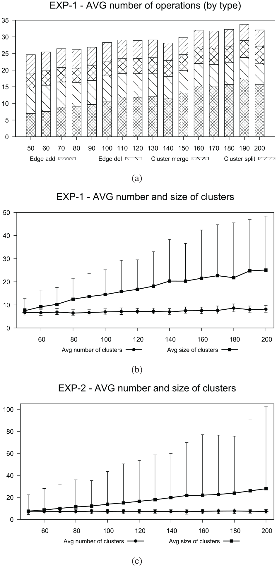
The test suite for EXP-1 is composed of $1120$ instances, each consisting of an initial graph (with an initial drawing) and a sequence of events. An event is either an edge addition operation or an edge removal operation, which may imply an additional merging or splitting operation. For every $n \in {50, 60, 70, \dots, 200}$ , we generate $70$ instances each consisting of a graph with $n$ vertices and a sequence of events (edge addition/deletion) that guarantees exactly $10$ merging/splitting operations. On average, the number of operations is about $30$ . The chart in Figure 8(a) shows the average number of operations for each value of $n$ , subdivided by type of operations.

Figure 8.

(a) Average number of operations subdivided by type in EXP-1 ( $y$ -axis), (b) average number and size (number of vertices) of connected components in EXP-1 ( $y$ -axis), and (c) average number and size of connected components in EXP-2 ( $y$ -axis). In (b) and (c), the error bars show maximum and minimum values; the minimum value for the cluster size is always 1, thus we do not show it. The $x$ -axis represents the number of vertices.

The instances are randomly generated as follows. We first generate an initial graph $G_{0}$ with $n$ vertices and $n$ edges, and we compute its connected components. To determine the initial layout of $G_{0}$ we randomly generate with uniform probability distribution the two linear orderings of the vertices along the $x$ -axis and along the $y$ -axis (for the 1D model the ordering along the $y$ -axis is ignored). In fact, since the online algorithm is not aware of the sequence of changes, there is no reason to prefer some specific vertex orderings. To generate the events, we repeatedly extract pairs of vertices. If the vertices of an extracted pair are adjacent in the graph we remove the edge (and thus we have an edge removal operation); if they are not adjacent we add the edge between them (and thus we have an edge addition operation). After the edge addition/removal is executed we update the set of connected components of the graph; if this set is changed, we add to the sequence of operations a component merge operation or a component split operation. With this generation procedure, we observed that extracting each pair of vertices with the same probability gives rise to an unbalanced situation where there is a giant component and several small components, and in this case the offline algorithm behaves very similarly to the online algorithm. This is because the giant component is never moved when a merge operation is performed. To make the set of experiments more meaningful, we modified the procedure so that it generates a sequence of events that guarantees a more balanced set of connected components. We select a pair of vertices with a probability that depends on the fact that the two vertices are adjacent or not; this probability is updated after each operation is generated. More precisely, let $u \in c_{i}$ and $v \in c_{j}$ be two vertices (notice that the two components $c_{i}$ and $c_{j}$ may coincide); we assign to the pair $u$ and $v$ a score equal to $n (c_{i}) / n$ if $u$ and $v$ are adjacent and to $1 - min {1, \frac{n (c_{i}) + n (c_{j})}{n}}$ if $u$ and $v$ are not adjacent. The scores are then normalized to be between $0$ and $1$ . Second, when the size (number of vertices) of a component $c$ is above a fixed threshold ( $n / 6$ in our case), the probability is set to $0$ for every pair of non-adjacent vertices that involves a vertex of $c$ . The rationale behind these probability values is that they dynamically increase the probability of splitting big components and, at the same time, reduce the probability of merging two components into a big one. Figure 8(b) shows the average number of clusters and their average size throughout the whole sequence of graphs. The edges for the initial graph $G_{0}$ are generated with the same probability-based strategy, but only considering edge additions. Observe that, the probabilities used to generate the sequence of events avoid that the number of clusters becomes too small or too big; this is why this number remains approximately constant on average.

The test suite for EXP-2 is generated with the same strategy as above, but only considering edge additions. More precisely, we generate a sequence of events that guarantees $4$ merging operations. The average number of operations is about $9$ . We also removed the threshold on the size of clusters, because, having only edge additions, the size of clusters can only grow and the generation algorithm may get stuck. We remark that generating instances with a higher number of merging operations often causes quite long running times for the offline algorithm, which prevents us from completing the whole set of experiments in a reasonable time. Also, we observed that executing EXP-2 was much more expensive in terms of computational time than executing EXP-1. This is due to the fact that, having only merging operations, the clusters are bigger and the value of the optimal solution is higher. As a consequence, the upper bound on the value of the solution used to avoid the exploration of subtrees that cannot lead to the optimal solution is also higher and therefore less effective in reducing the exploration of the tree of candidate solutions. For this reason, we limited EXP-2 to 20 instances (instead of 70) for each fixed value of $n$ . Figure 8(c) shows the average number of clusters and the average size of the clusters for this second test suite.

Experimental comparison

In each experiment we compare the online algorithm for the 1D and 2D drawing models against the offline algorithm. For the 1D drawing model we study both the case when the offline algorithm minimizes the total stability cost and the case when it minimizes the maximum stability cost. For the 2D drawing model we only consider the minimization of the total stability cost, because for this model the execution of the offline algorithm to minimize the maximum cost turned out to be computationally too expensive. Namely, if we want to minimize the maximum stability cost in 2D, we cannot optimize independently the ordering of the vertices along the $x$ -direction and along the $y$ -direction. Thus, when considering a merge operation the number of possibilities to consider would be quadratic in the number of connected components rather than linear.

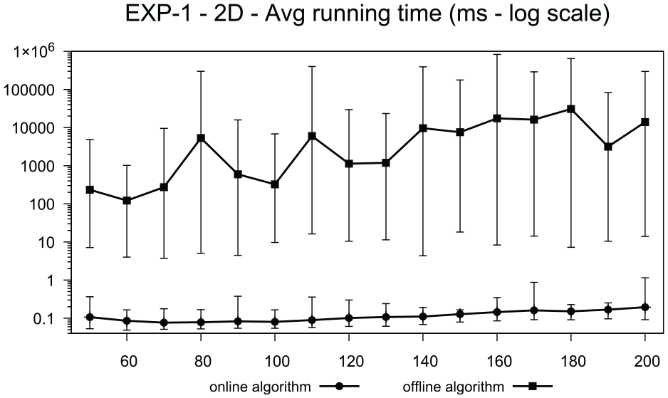
In terms of running time, for every instance the online algorithm is very fast and takes less than 1.15 ms. On the other hand, the offline algorithm is much more expensive and can even take several minutes. For example, the chart in Figure 9 shows the average running time of the two algorithms on EXP-1 and for the 2D drawing model. The results for EXP-2 and for the 1D drawing model are similar, thus we do not report the corresponding charts.

Figure 9.

Average running time (with logarithmic scale) of the two algorithms on EXP-1 and for the 2D drawing model ( $y$ -axis). The error bars show minimum and maximum values. The $x$ -axis represents the number of vertices.

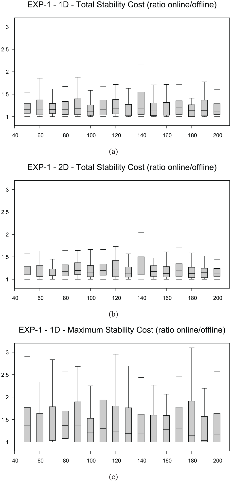
Concerning the stability cost, Figure 10 reports the data about EXP-1 for the two drawing models. In particular, for each value of $n \in {50, 60, 70, \dots, 200}$ , the charts show the distribution (summarized by means of box and whisker plots) of the ratio between the value of the solution of the online algorithm and the value of the optimal solution. The charts show a similar behavior: The total stability cost of the online algorithm approximates that of the offline algorithm by a factor of $1.23$ on average both in the 1D and in the 2D drawing model; the factor is $1.5$ on average for the maximum stability cost. The similarity of the experimental approximation factors in the 1D and 2D cases reflects the fact that our algorithmic strategy handles the 2D case by independently solving two 1D optimization problems, one for the $x$ -axis and one for the $y$ -axis.

Figure 10.

EXP-1: (a) distribution of the ratio between the total stability cost of the two algorithms for the 1D drawing model ( $y$ -axis), (b) distribution of the ratio between the total stability cost of the two algorithms for the 2D drawing model ( $y$ -axis), and (c) distribution of the ratio between the maximum stability cost of the two algorithms for the 1D drawing model( $y$ -axis). The $x$ -axis represents the number of vertices.

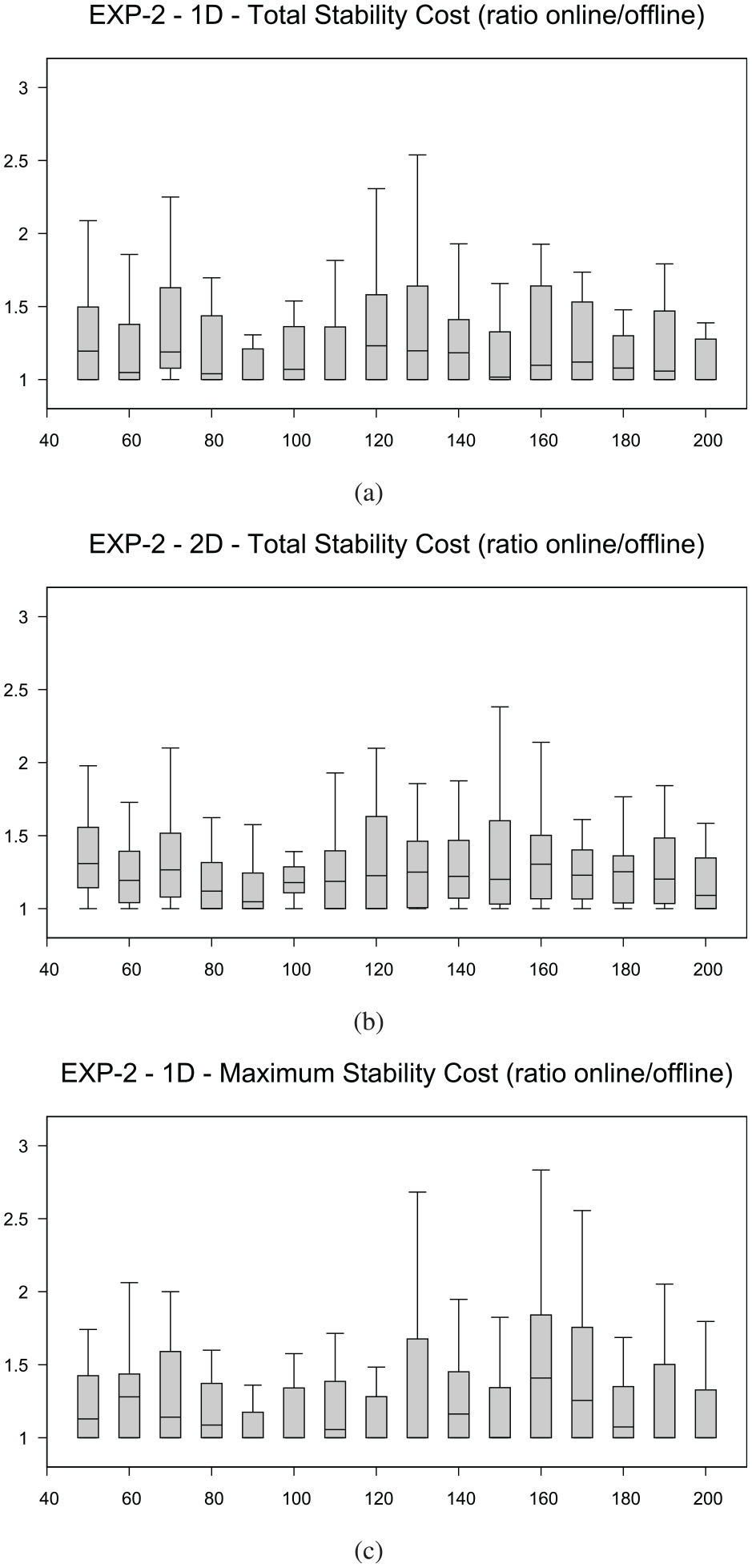
Figure 11 reports the distributions of the ratio of the stability costs for EXP-2. The charts show a behavior similar to that in Figure 10; in this case the average approximation factors are $1.29$ for the total stability cost both in 1D and in 2D, and $1.28$ for the maximum stability cost in 1D.

Figure 11.

EXP-2: (a) distribution of the ratio between the total stability cost of the two algorithms for the 1D drawing model ( $y$ -axis), (b) distribution of the ratio between the total stability cost of the two algorithms for the 2D drawing model ( $y$ -axis), and (c) distribution of the ratio between the maximum stability cost of the two algorithms for the 1D drawing model( $y$ -axis). The $x$ -axis represents the number of vertices.

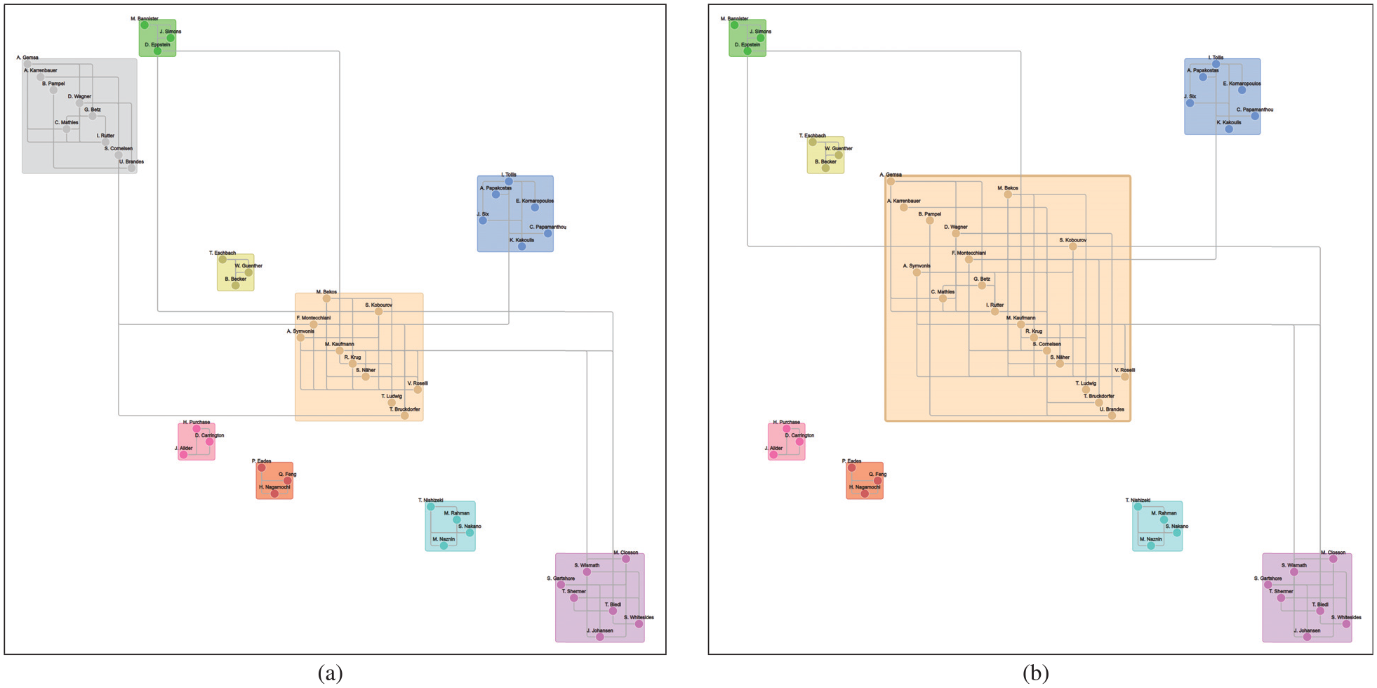
Table 1 reports the number of instances for which the online algorithm matches the cost of the offline algorithm, that is, those for which it reaches the optimum value. One can notice that the number of hits is larger for EXP-2 when there are only merge operations. This can be explained by observing that the solution space becomes larger if the sequence of operations includes both merging and splitting components. Namely, when there are only merge operations the number of clusters is smaller and their size is larger (see also Figure 8(c)).

Table 1.

Number of instances for which the online algorithm matches the optimum value.

	EXP-1	EXP-2
1D total cost	184 (16%)	141 (44%)
2D total cost	52 (4%)	73 (23%)
1D max cost	341 (30%)	157 (49%)

Case study

As a proof-of-concept of our online visualization approach, we tested it on a dynamic collaboration network constructed from real data. Since we have free low-level access to the database of the Journal of Graph Algorithms and Applications (JGAA) (http://jgaa.info/), we opted for extracting information from it. In order to limit the scope of our case study, we decided to focus on a subset of papers in this database, namely those devoted to the specific topic “orthogonal drawing”. We chose this topic because it has a long tradition in graph visualization and involves JGAA publications that span a relatively long time window. We determined the relationships between the authors of these papers in terms of their collaborations, according to the following model. Denote by $A$ the set of extracted authors. For each pair ${u, v}$ of authors in $A$ sharing some JGAA paper $p$ , we created in the collaboration network a temporal edge $(u, v)$ having a starting date $s_{p}$ and an ending date $t_{p}$ . This temporal edge represents the life-time of the collaboration between $u$ and $v$ determined by $p$ . The ending date $t_{p}$ coincides with the publication date of $p$ , while the starting date $s_{p}$ is defined as $s_{p} = t_{p} - c \cdot σ_{p}$ , where $σ_{p}$ is the number of pages of $p$ and $c$ is a positive constant that expresses a given number of weeks. According to this model, the life-time of the collaboration between $u$ and $v$ determined by $p$ is directly proportional to the number of pages (i.e. the size) of $p$ , which is a reasonable assumption. In particular, we fixed $c = 3$ . If at any time from $s_{p}$ to $t_{p}$ another collaboration between $u$ and $v$ starts, due to a paper $p'$ , the ending date of edge $(u, v)$ is updated to $max {t_{p}, t_{p'}}$ . The resulting network contains $56$ vertices and $98$ edges in the whole time window, determined by a total of $48$ papers.

To visually analyze the evolution of this network we implemented a graphical interface that adopts our 2D model for the series of drawings $Γ_{0}, \dots, Γ_{k}$ , representing the series of graphs $G_{0}, \dots, G_{k}$ . In this interface, the transition from $Γ_{i}$ to $Γ_{i + 1}$ exploits a simple animation, depending on the type of event. When a new edge $(u, v)$ is inserted, the following sequence of actions is executed: $(i)$ the borders of vertices $u$ and $v$ are highlighted for a short time (e.g. 1 s); $(ii)$ edge $(u, v)$ is physically drawn; $(iii)$ if $u$ and $v$ did not belong to the same cluster (component), the border of their clusters are highlighted for a short time and then the two clusters are merged. Since our online algorithm places the new cluster in-between the previous two, this animation generally suffices to quickly recognize the merged cluster at the end of the process. When an edge $(u, v)$ is removed, the sequence of actions is as follows: $(i)$ edge $(u, v)$ is highlighted for a short time; $(ii)$ edge $(u, v)$ is physically deleted from the drawing; $(iii)$ if the removal of $(u, v)$ causes the split of the cluster of $u$ and $v$ into two clusters, all the vertices of one of these two clusters are highlighted for a short time and then the cluster is split.

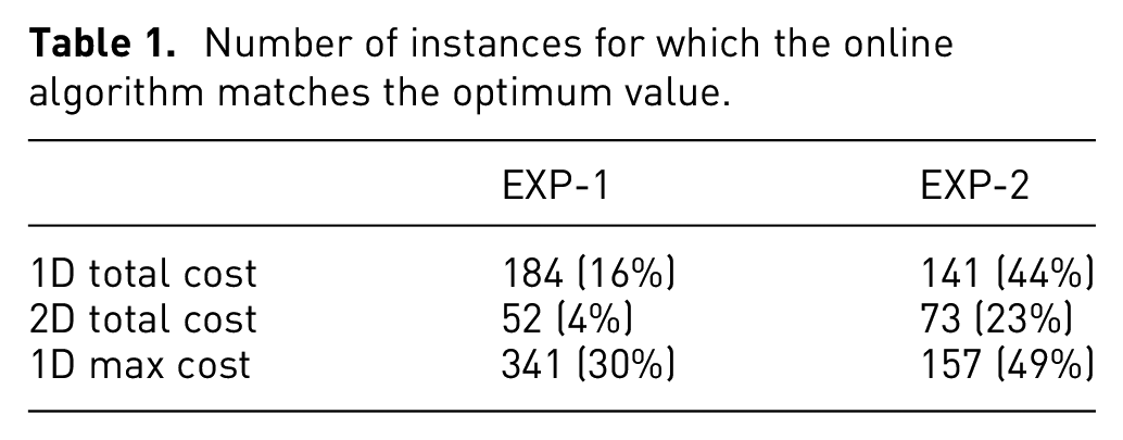
The analysis of the dynamic network started from a situation in which there was no relationship between authors. During an initial phase of the evolution we progressively observed the formation of several small connected components, consisting of up to four vertices. We noted that each component clearly represented a well distinct group of authors working in a specific geographic area; for example, we could observe the three components {Eades, Feng, Nagamochi}, {Biedl, Shermer, Whitesides, Wismath}, and {Kakoulis, Papakostas, Six, Tollis}. Merging and splitting operations of small components were observed for a considerable portion of the time window (approximatively until $1 / 3$ of the evolution). Then, we progressively observed to the formation of few bigger components; in particular, at a time corresponding to about $2 / 3$ of the time window we could identify two main distinct connected components, one consisting of $9$ vertices and the other consisting of $5$ vertices. These components reflected two different communities, with the majority of researchers from Germany. After a while, these two components were merged together, due to new collaborations between subsets of their elements, for example, a collaboration between Rutter (who belonged to the community with $5$ vertices) and Bekos (who belonged to the community with $9$ vertices). We verified that this new collaboration was on a paper about boundary labeling, a topic strictly related to orthogonal drawings. In the remaining part of the time window this new big component grew up to about $20$ vertices. In the tail of the evolution we observed several splitting operations, which witnessed the end of the collaborations in the considered time window. Figure 12 reports a portion of the visualization generated by our interface in two different time instants, namely immediately before and immediately after the merging of the two aforementioned components with $5$ and $9$ vertices, respectively. A video showing an animation of this network is available at https://www.youtube.com/watch?v=fAx-4b69Vbw.

Figure 12.

Two consecutive time instants of a portion of the JGAA evolving network. Passing from (a) to (b) two components have been merged due to the insertion of an edge between Bekos and Rutter.

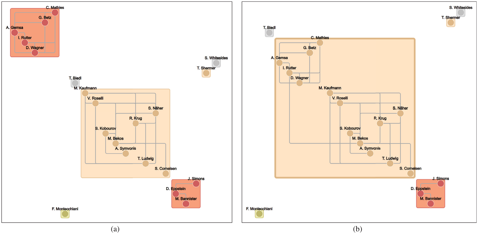
We finally remark that our algorithmic approach can be applied to the visualization of dynamic networks where clusters do not necessarily coincide with the connected components of the graph, but are determined by some automatic clustering algorithm that uses only cluster split and cluster merge operations. For example, Figure 13 shows the visualization (by means of our interface) of a co-authorship network (with a subset of authors in the previous example, but with different types of relationships) in two different time instants, where clusters represent denser portions of the network. The two time instants still refer to the situation before and after a merging operation.

Figure 13.

Two consecutive time instants of a dynamic co-authorship network, where clusters do not coincide with the connected components.

Concluding remarks

We presented two models for dynamic visualization of graphs, focusing on highlighting the different connected components of the graph. For these models, we described online algorithms that aim to maximize the drawing stability over a sequence of events. We reported the results of an experimental study that showed good performance of the online algorithm when compared to an offline algorithm that knows the whole sequence of events in advance. Also, as a proof-of-concept of our approach, we described a case study on a real network performed by means of a graphical interface that animates the sequence of graph changes through our online algorithms. We conclude with some theoretical and application remarks.

Theoretical remarks

Lemma 2 shows that in theory the online solution can be arbitrarily worse than the offline solution. An intermediate strategy can be studied where the updates on the drawing are executed only after a certain number of steps; this number can be regarded as a parameter of a visual analytics system for dynamically evolving networks. Such intermediate strategies should have a positive impact on the running times and it may avoid the worst case effect of Lemma 2.

As a second remark, our offline strategy has a time complexity that is exponential in the number of merging/splitting operations. We find it interesting to study the complexity of the offline problem, namely is it possible to design a polynomial-time offline algorithm or is this optimization task NP-hard? In the second case, is there any (offline) approximation algorithm?

We finally mention the possibility of studying variants of our drawing stability cost function, where not only the number of pairs of vertices that change their relative ordering is considered but also the specific vertices involved over all these pairs. For example, suppose that $u, v, w, z$ are four vertices that occur in this linear ordering. According to our cost function, the new ordering $v, w, z, u$ would cost 3 while the ordering $v, u, z, w$ would cost 2. However, the first ordering may be judged more stable than the second one, because each costly pair involves $u$ . Similar considerations can be found in the literature about how to evaluate the visual complexity of a graph layout. For example, counting the number of block crossings (pairs of intersecting bundles of edges) has been proposed as an alternative to counting the number of edge crossings.^60,61

Application remarks

Our theoretical model has some clear limits in terms of its applicability. It is specifically conceived to analyze the evolution of some types of dynamic relationships over a target set of vertices. Extensions to a broader set of scenarios can be considered. For example, one can assume that also a single vertex may appear or disappear at every time instant. In our algorithmic approach, the addition of a vertex easily corresponds to the addition of a trivial connected component, which can be added in any position of the current layout. On the contrary, the removal of a vertex $v$ causes the removal of all its incident edges, and therefore the potential fragmentation of a connected component into several ones. In this respect, an interesting problem is how to efficiently choose the removal order of the edges incident to $v$ that leads to the minimum cost. Another interesting extension is to consider more complex types of events such as the insertion/removal of multiple edges at a time. This would allow the analysis of dynamic phenomena at a coarser scale. Although such a complex event can be easily adapted to our model by breaking it down into a sequence of elementary events, a more global approach might lead to a more effective solution.

From the visualization point of view, we observe that the algorithms for the 1D drawing model can be naturally applied to circular drawings and to chord diagrams. Also, as already observed in the previous sections, our drawing models and strategies can be used for the visualization of dynamic clustered graphs where clusters do not necessarily coincide with connected components. In this case, the possible presence of edges that join two clusters may suggest to optimize additional criteria other than the vertex/cluster stability. For example, one can try to minimize edge stress⁵² so that clusters connected by many edges are closer in the visualization than weakly connected clusters. Finally, we observed that the area requirement of L-drawings is high and does not allow the visualization of large graphs. It is interesting to investigate more compact types of layouts that keep subdrawings within the bounding box of their vertices, while keeping the drawing stable at each edge insertion/removal.

Footnotes

Acknowledgements

This work started at the Shonan Meeting: “Reimagining the Mental Map and Drawing Stability”, 10th-13th, 2018. We acknowledge the organizers of the workshop and the anonymous reviewers of this manuscript for their valuable comments and suggestions.

Funding

The author(s) disclosed receipt of the following financial support for the research, authorship, and/or publication of this article: This work was partially supported by the project MIUR, Grant 20174LF3T8 “AHeAD: efficient Algorithms for HArnessing networked Data.

ORCID iD

Walter Didimo

References

Newman

Barabasi

A-L

Watts

DJ.

The structure and dynamics of networks: Princeton studies in complexity. Princeton, NJ, USA: Princeton University Press, 2006.

Beck

Burch

Diehl

Weiskopf

A taxonomy and survey of dynamic graph visualization. Comput Graph Forum 2017; 36(1): 133–159.

Misue

Eades

Lai

Sugiyama

Layout adjustment and the mental map. J Vis Lang Comput 1995; 6(2): 183–210.

Purchase

Hoggan

Görg

. How important is the “mental map”? - an empirical investigation of a dynamic graph layout algorithm. In: Graph drawing, volume 4372 of lecture notes in computer science. New York: Springer, 1996, pp.184–195.

Archambault

Purchase

Pinaud

Animation, small multiples, and the effect of mental map preservation in dynamic graphs. IEEE Trans Vis Comput Graph 2011; 17(4): 539–552.

Archambault

Purchase

. The mental map and memorability in dynamic graphs. In: PacificVis’12, pp.89–96. IEEE Computer Society, 2012.

Archambault

Purchase

HC.

The “Map” in the mental map: experimental results in dynamic graph drawing. Int J Hum Comput Stud 2013; 71(11): 1044–1055.

Federico

Miksch

. Evaluation of two interaction techniques for visualization of dynamic graphs. In: Graph drawing, volume 9801 of lecture notes in computer science. New York: Springer, 2016, pp.557–571.

Lezama

Chounta

Göhnert

Hoppe

HU.

Visual stability in dynamic graph drawings. i-com 2015; 14(3): 220–230.

10.

Wattenberg

Arc diagrams: visualizing structure in strings. In: INFOVIS, pp.110–116. IEEE Computer Society, 2002.

11.

Angelini

Da Lozzo

Di Bartolomeo

, et al. Algorithms and bounds for L-drawings of directed graphs. Int J Found Comput Sci 2018; 29(4):461–480.

12.

Duncan

Goodrich

MT.

Planar orthogonal and polyline drawing algorithms. In: Handbook of graph drawing and visualization. New York: Chapman and Hall/CRC, 2013, pp.223–246.

13.

Frishman

Tal

. Dynamic drawing of clustered graphs. In: INFOVIS, pp.191–198. IEEE Computer Society, 2004.

14.

Brandes

Corman

SR.

Visual unrolling of network evolution and the analysis of dynamic discourse?

Inform Vis 2003; 2(1): 40–50.

15.

Burch

Vehlow

Beck

Diehl

Weiskopf

Parallel edge splatting for scalable dynamic graph visualization. IEEE Trans Vis Comput Graph 2011; 17(12): 2344–2353.

16.

Greilich

Burch

Diehl

Visualizing the evolution of compound digraphs with timearctrees. Comput Graph Forum 2009; 28(3): 975–982.

17.

Shi

Wang

Wen

Lin

Liao

1.5d Egocentric dynamic network visualization. IEEE Trans Vis Comput Graph 2015; 21(5): 624–637.

18.

van den Elzen

Holten

Blaas

van Wijk

. Dynamic network visualization withextended massive sequence views. IEEE Trans Vis Comput Graph 2014; 20(8): 1087–1099.

19.

Köpp

Weinkauf

Temporal treemaps: static visualization of evolving trees. IEEE Trans Vis Comput Graph 2018; 25(1): 534–543.

20.

Frishman

Tal

Online dynamic graph drawing. IEEE Trans Vis Comput Graph 2008; 14(4): 727–740.

21.

Gorochowski

di Bernardo

Grierson

CS.

Using aging to visually uncover evolutionary processes on networks. IEEE Trans Vis Comput Graph 2012; 18(8): 1343–1352.

22.

Diehl

Görg

Kerren

. Preserving the mental map using foresighted layout. In: VisSym, pp.175–184. Eurographics Association, 2001.

23.

Feng

Wang

Shen

Lee

Coherent time-varying graph drawing with multifocus+context interaction. IEEE Trans Vis Comput Graph 2012; 18(8): 1330–1342.

24.

Görg

Birke

Pohl

Diehl

. Dynamic graph drawing of sequences of orthogonal and hierarchical graphs. In: Graph drawing, volume 3383 of lecture notes in computer science. New York: Springer, 2004, pp.228–238.

25.

Eiglsperger

Gutwenger

Kaufmann

, et al. Automatic layout of UML class diagrams in orthogonal style. Inf Vis 2004; 3(3): 189–208.

26.

Vehlow

Beck

Weiskopf

Visualizing dynamic hierarchies in graph sequences. IEEE Trans Vis Comput Graph 2016; 22(10): 2343–2357.

27.

Vehlow

Beck

Weiskopf

Visualizing group structures in graphs: a survey. Comput Graph Forum 2017; 36(6): 201–225.

28.

Dogrusöz

Two-dimensional packing algorithms for layout of disconnected graphs. Inf Sci 2002; 143(1–4): 147–158.

29.

Freivalds

Dogrusöz

Kikusts

. Disconnected graph layout and the polyomino packing approach. In: Graph drawing, volume 2265 of lecture notes in computer science. New York: Springer, 2001, pp.378–391.

30.

Goehlsdorf

Kaufmann

Siebenhaller

. Placing connected components of disconnected graphs. In: APVIS, pp.101–108. IEEE Computer Society, 2007.

31.

von Landesberger

Görner

Schreck

. Visual analysis of graphs with multiple connected components. In IEEE VAST, pp.155–162. IEEE Computer Society, 2009.

32.

Gansner

North

SC.

Interactive visualization of streaming text data with dynamic maps. J Graph Algorithms Appl 2013; 17(4): 515–540.

33.

Gansner

Efficient node overlap removal using a proximity stress model. In: Graph drawing, volume 5417 of lecture notes in computer science. New York: Springer, 2008, pp.206–217.

34.

Bridgeman

Tamassia

Difference metrics for interactive orthogonal graph drawing algorithms. J Graph Algorithms Appl 2000; 4(3): 47–74.

35.

Nicholson

TAJ

. Permutation procedure for minimising the number of crossings in a network. Proc Inst Electr Eng 1968; 115: 2126.

36.

Saaty

The minimum number of intersections in complete graphs. Proc Natl Acad Sci USA 1964; 52(3): 688–690.

37.

Masuda

Nakajima

Kashiwabara

Fujisawa

Crossing minimization in linear embeddings of graphs. IEEE Trans Comput 1990; 39(1): 124–127.

38.

Bernhart

Kainen

PC.

The book thickness of a graph. J Combin Theory Ser B 1979; 27(3): 320–331.

39.

Binucci

Di Giacomo

Hossain

Liotta

1-page and 2-page drawings with bounded number of crossings per edge. Eur J Combin 2018; 68: 24–37.

40.

Cimikowski

Algorithms for the fixed linear crossing number problem. Discrete Appl Math 2002; 122(1–3): 93–115.

41.

Cimikowski

Shope

A neural-network algorithm for a graph layout problem. IEEE Trans Neural Netw 1996; 7(2): 341–345.

42.

Skora

Vrt’o

Crossing minimisation heuristics for 2-page drawings. Electron Notes Discrete Math 2005; 22: 527–534.

43.

Klawitter

Mchedlidze

Nöllenburg

. Experimental evaluation of book drawing algorithms. In: Graph drawing, volume 10692 of lecture notes in computer science. Springer, 2017, pp.224–238.

44.

Pretorius

van Wijk

JJ.

Bridging the semantic gap: visualizing transition graphs with user-defined diagrams. IEEE Comput Graph Appl 2007; 27(5): 58–66.

45.

Gansner

Koren

Improved circular layouts. In: Graph drawing, volume 4372 of lecture notes in computer science. New York: Springer, 2006, pp.386–398.

46.

Krzywinski

Schein

Birol

, et al. Circos: an information aesthetic for comparative genomics. Genome Res 2009; 19(9): 1639–1645.

47.

Six

Tollis

IG.

Circular drawing algorithms. In: Handbook of graph drawing and visualization. New York: Chapman and Hall/CRC, 2013, pp.285–315.

48.

Arleo

Didimo

Liotta

Montecchiani

Profiling distributed graph processing systems through visual analytics. Future Generation Comp Syst 2018; 87:43–57.

49.

Gronemann

Jünger

Liers

Mambelli

Crossing minimization in storyline visualization. In: Graph drawing, volume 9801 of lecture notes in computer science. Springer, 2016, pp.367–381.

50.

Kostitsyna

Nöllenburg

Polishchuk

Schulz

Strash

. On minimizing crossings in storyline visualizations. In: Graph drawing, volume 9411 of lecture notes in computer science. Springer, 2015, pp.192–198.

51.

Di Battista

Eades

Tamassia

Tollis

. Graph drawing: algorithms for the visualization of graphs. Upper Saddle River: Prentice-Hall, 1999.

52.

Kaufmann

Wagner

(eds). Drawing graphs, methods and models (The book grow out of a Dagstuhl Seminar, April 1999), volume 2025 of lecture notes in computer science. New York: Springer, 2001.

53.

Kieffer

Dwyer

Marriott

Wybrow

HOLA: human-like orthogonal network layout. IEEE Trans Vis Comput Graph 2016; 22(1): 349–358.

54.

Batagelj

Brandenburg

Didimo

Liotta

Palladino

Patrignani

Visual analysis of large graphs using (X, Y)-clustering and hybrid visualizations. IEEE Trans Vis Comput Graph 2011; 17(11): 1587–1598.

55.

Di Battista

Didimo

Marcandalli

. Planarization of clustered graphs. In: Graph drawing, volume 2265 of lecture notes in computer science. New York: Springer, 2001, pp.60–74.

56.

Di Giacomo

Didimo

Liotta

Palladino

. Visual analysis of one-to-many matched graphs. J Graph Algorithms Appl 2010; 14(1): 97–119.

57.

Eades

Feng

Nagamochi

Drawing clustered graphs on an orthogonal grid. J Graph Algorithms Appl 1999; 3(4): 3–29.

58.

Auber

Bonichon

Dorbec

Pennarun

Rook-drawings of plane graphs. J Graph Algorithms Appl 2017; 21(1): 103–120.

59.

Biedl

Pennarun

Non-aligned drawings of planar graphs. J Graph Algorithms Appl 2017; 21(5): 915–937.

60.

Chaplick

van Dijk

Kryven

Park

Ravsky

Wolff

. Bundled crossings revisited. In: Graph drawing, volume 11904 of lecture notes in computer science. New York: Springer, 2019, pp.63–77.

61.

van Dijk

Fink

Fischer

, et al. Block crossings in storyline visualizations. J Graph Algorithms Appl 2017; 21(5): 873–913.