Out-of-sample data visualization using bi-kernel t-SNE

Abstract

T-distributed stochastic neighbor embedding (t-SNE) is an effective visualization method. However, it is non-parametric and cannot be applied to steaming data or online scenarios. Although kernel t-SNE provides an explicit projection from a high-dimensional data space to a low-dimensional feature space, some outliers are not well projected. In this paper, bi-kernel t-SNE is proposed for out-of-sample data visualization. Gaussian kernel matrices of the input and feature spaces are used to approximate the explicit projection. Then principal component analysis is applied to reduce the dimensionality of the feature kernel matrix. Thus, the difference between inliers and outliers is revealed. And any new sample can be well mapped. The performance of the proposed method for out-of-sample projection is tested on several benchmark datasets by comparing it with other state-of-the-art algorithms.

Keywords

Data visualization dimensionality reduction T-SNE out-of-sample extension outlier projection

Introduction

The recent development in information technologies has led to an astonishing increase in the amount of data stored and consumed.¹ Visualization of high-dimensional data is one of the most important and fundamental tasks in big data handling, offering an intuitive interface to rapidly detect the structural elements of data, such as clusters or outliers.^2,3

Dimensionality reduction (DR) techniques are widely used for high-dimensional data visualization, such as principal component analysis (PCA),^4–6 locally linear embedding,^7,8 isometric feature mapping^9,10 and t-distributed stochastic neighbor embedding (t-SNE).¹¹ However, some of these methodologies are only used for supervised learning, and some are linear or non-parametric methods, with their own set of advantages and disadvantages in solving different problems.¹²

T-SNE is one of the most effective nonlinear data visualization technologies. It can keep the low-dimensional features of similar high-dimensional pairs as close as possible so that the natural clusters of the original data are presented.¹³ T-SNE has been successfully applied to visualize different types of data such as handwritten digital data,¹⁴ genomic data,¹⁵ engine vibration signals,¹⁶ chemical process data,¹⁷ and specimen thermograms.¹⁸ However, t-SNE has limitations for out-of-sample extension because of its non-parametric characteristic.¹⁹ Once the given samples are mapped, it is difficult to extend the mapping to new data points. In other words, t-SNE yields a new result every time a new data point is added, making it inapplicable for online data visualization. Even through several out-of-sample extensions of t-SNE have been proposed in the last few years, they still have drawbacks in outlier projection, computational time, or parametric selection.

To address the above problems, bi-kernel t-SNE is proposed for out-of-sample data visualization. The kernel functions of both the high-dimensional input data and the low-dimensional features are used to approximate the projections. PCA is then applied to reduce the dimensionality of the feature kernel matrix to two for visualization. With the bi-kernel mapping and PCA, outliers are depicted away from inliers in the two-dimensional (2D) scatter plots. The contribution of bi-kernel t-SNE is that it realizes an out-of-sample extension for t-SNE with few parameters and yields convincing inlier and outlier projections in linear time.

The rest of the paper is structured as follows. Section 2 briefly introduces some concepts about dimensionality reduction techniques. Section 3 reviews the original t-SNE and its several out-of-sample extensions. Section 4 details bi-kernel t-SNE, which is proposed based on kernel t-SNE and PCA. Evaluation measures for inlier and outlier mapping are introduced in Section 5. In Section 6, the effectiveness of bi-kernel t-SNE is illustrated with experimental results. Section 7 provides the discussion of the results. Section 7 concludes the paper.

Dimensionality reduction

In data visualization techniques, high-dimensional samples are mapped to a 2D space for visualization while preserving the data structure as much as possible.²⁰ Consider a dataset X = ( x ₁, x ₂,…, x _n)^T, where x _i (1≤i≤n) is an m-dimensional observation or sample, and its low-dimensional embedding Y = ( y ₁, y ₂,…, y _n) ^T, where y _j (1≤j≤n) is a q-dimensional feature. T means the transposed of the matrix. A DR technique is then a function²¹

f : X (x_{i} \in R^{m}, 1 \leq i \leq n) \to Y (y_{j} \in R^{q}, 1 \leq j \leq n)

(1)

where q≪m, and typically q = 2.

Among the numerous DR techniques, many of them are non-parametric. Thus, out-of-sample data cannot be incorporated into the existing projection. Parametric projection techniques provide an explicit way to express the function f. When new samples come, they can be directly mapped with the learned function f.

In this study, we define that out-of-sample data has two categories: inlier and outlier. An inlier has the same label with the training samples or belongs to some structure in the original space. Outliers have different labels from all training samples. For inlier projection, the 2D embedding should belong to one of the training clusters. For outliers, the 2D projection should be separated from the training embedding. Ideally, the classes in outliers should be separated in the 2D map and far from the training regions in the meantime. However, many out-of-sample data projection methods only focus on inlier projection.

To evaluate a DR technique, both inlier and outlier projections should be discussed. There is no doubt that data visualization is a good way to show the existing clusters and outliers. However, we still need several indicators to gauge different properties of a DR technique in a quantitative way. Reviews of different quality metrics have been reported in many literatures.^21–24 In this study, five quality metrics are used for inlier projection evaluation to see how well the projection can separate the clusters and how well the parametric projection can mimic the ground-truth projection. For outlier projection, we use the well-known F1 score and area under curve (AUC) to evaluate the performance. The evaluation measures for both inlier and outlier mappings used in this study are detailed in section 5.

T-SNE and its out-of-sample extensions

In this section, we first introduce t-SNE briefly and then discuss its several out-of-sample extensions.

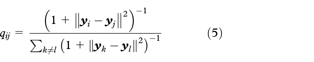
As an unsupervised nonlinear DR technique, t-SNE calculates the similarity with conditional probabilities. It captures the local structure of the high-dimensional data very well, while also revealing the global structure.¹³ It uses a symmetrized cost function with simple gradients and a student-t-distribution to compute the similarity in the low-dimensional space, solving the “difficult to optimize problem” and the “crowding problem” observed in SNE. The cost function, that is, KL divergence, is computed as

C = KL (P | | Q) = \sum_{i} \sum_{j} p_{ij} \log \frac{p_{ij}}{q_{ij}}

(2)

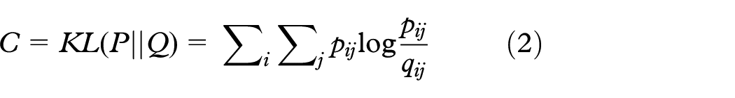
where P and Q are the joint probability distributions in the high-dimensional and low-dimensional spaces, respectively. Taking x as the input high-dimensional data point, we can compute the joint probabilities p_ij with Gaussian distribution, which are defined as

p_{ij} = \frac{p_{j | i} + p_{i | j}}{2 n}

(3)

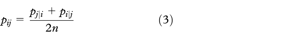
where n is the number of samples. $p_{j | i}$ is the symmetrized conditional probability with a parameter σ_i. In t-SNE, σ_i is determined with a fixed perplexity using a binary search technique. The perplexity is typically set to a value between 5 and 50.¹³

Perp (i) = 2^{- \sum_{j, i \neq j} p_{j | i} lo g_{2} (p_{j | i})}

(4)

Taking y as the low-dimensional feature, we can compute the joint probabilities q_ij with the student-t-distribution, which is defined as

q_{ij} = \frac{{(1 + {‖ y_{i} - y_{j} ‖}^{2})}^{- 1}}{\sum_{k \neq l} {(1 + {‖ y_{k} - y_{l} ‖}^{2})}^{- 1}}

(5)

The objective of t-SNE is to find the optimal y by minimizing the KL divergence via the gradient descent technique.¹³

The main limitation of t-SNE is that it is a non-parametric technique.¹⁹ Once the given samples are mapped, it is difficult to extend the mapping to new data points. To overcome this drawback, some attempts have been made to extend t-SNE for out-of-sample projection.

Neural networks (NN) can learn many complex functions, including the t-SNE projection. Van Der Maaren²⁵ used restricted Boltzmann machines to learn an explicit projection between $R^{m}$ and $R^{2}$ , which is known as parametric t-SNE (pt-SNE). However, parameter choosing is a tricky problem for pt-SNE. The training requires lots of data and is time-consuming. Espadoto et al.²¹ used a deep learning (DL) method to learn any projection methods, including t-SNE. The neural network has three fully connected hidden layers and a two-element output layer. The three fully connected hidden layer have 256, 512 and 256 units, respectively, where ReLU activation functions are used. Sigmoid activation function is applied in the output layer. One common problem of NN-based t-SNE is that outliers are not well projected. In literature,²¹ it is mentioned that fine-tuning the trained NN with a small group of unrelated samples can lead to a good result. Zhu et al.²⁶ generated additional dummy data to fine tune a reformulated-structured pt-SNE for outlier mapping to realize good industrial process data visualization. However, how to generate additional unrelated data for fine-tuning is still a great challenge.

Gisbrecht et al.¹⁹ proposed kernel t-SNE, where low-dimensional features can be approximately mapped by a linear combination of normalized Gaussian kernels of high-dimensional data points. It retains the flexibility of the basic t-SNE and enables an explicit out-of-sample extension in linear computing time. Kernel t-SNE can be considered as one of the interpolation methods, where the weights are derived from kernel mapping instead of some distance. However, outliers are still not well projected with interpolation methods.

Boytsov et al.²⁷ proposed local interpolation with outlier control t-SNE (LION t-SNE) to incorporate both inliers and outliers. It is based on local interpolation in the vicinity of training data, outlier detection and a special outlier mapping algorithm. Outlier detection is applied firstly to determine if the new sample is an outlier. If it is not an outlier, inverse distance weighted interpolation is used to place the projection in the vicinity of some y . If it is an outlier, the embedding is placed outside of the existing projection area. However, outlier detection and k nearest neighbors search are required for every new sample in the testing procedure of LION t-SNE, which is very time-consuming in practice.

Bi-kernel t-SNE

We discussed t-SNE and its several parametric variants in Section 3. Although these variants realize out-of-sample extension for t-SNE, they still have drawbacks in outlier projection, parameter selection, or computational time. To alleviate these problems, we present bi-kernel t-SNE in this section. It is proposed based on kernel t-SNE and PCA. Kernel t-SNE yields a simple out-of-sample extension with the kernel mapping. However, the mapping is performed directly on low-dimensional feature, which leads to a poor outlier projection. In bi-kernel t-SNE, the projection is approximated with the kernel functions of both the input data and the features. Then the dimensionality of the feature kernel matrix is reduced to two by PCA. With the bi-kernel mapping and PCA, outliers are mapped away from the existing region in the 2D scatter plots.

In this section, we firstly introduce kernel t-SNE and its drawbacks in outlier projection. Then we present the procedure of PCA. Finally, we propose bi-kernel t-SNE, together with a practical way for its parameter selection.

Kernel t-SNE

Kernel t-SNE was proposed to yield a simple out-of-sample extension for t-SNE with the kernel mapping. Denoting X and Y as the matrices of raw data x and the feature y , we can express the mapping from X to Y by a linear combination of the normalized Gaussian matrix of X¹⁹:

Y = A K_{x}

(6)

where the elements in the matrix K_x are calculated as

{[K_{x}]}_{i, j} = \frac{k (x_{i}, x_{j})}{\sum_{l} k (x_{i}, x_{l})} = \frac{\exp (- 0.5 ‖ x_{i} - x_{j} ‖^{2} / σ_{j}^{2})}{\sum_{l} \exp (- 0.5 ‖ x_{i} - x_{l} ‖^{2} / σ_{l}^{2})}

(7)

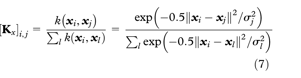
The parameter matrix A is obtained by

A = {(K_{x}^{T} K_{x})}^{- 1} K_{x}^{T} Y

(8)

For the out-of-sample extension, the standard t-SNE is first used to map X to obtain the training features. Gaussian kernel is then applied for explicit projection approximation. The parameter matrix A is obtained. When a new sample x _new arrives, the Gaussian kernel k _x,new is calculated and multiplied with A. The feature y _new is obtained in linear time.

Note that if the new sample is an outlier, the Gaussian kernel k _x,new will be extremely small or even near zero. After multiplying it with A, y _new may be near the origin, mixing with the inliers. This shows that kernel t-SNE is unsuitable for outlier mapping.

PCA

PCA is one of the most widely-used DR method and has been used for outlier detection in many fields. The main idea of it is to project data to a new orthogonal coordinate system. The dimensionality of data is reduced by only choosing the first few principal components, while preserving as much data variation as possible.

Given a data matrix $X = {(x_{1}, x_{2}, \dots, x_{n})}^{T} \in R^{m}$ , where x _i (1≤i≤n) contains m variables. The procedure of PCA reducing the dimensionality of X is as follows.²⁸

(1) Normalize X with the means and variances.

X' = \frac{X - μ}{σ}

(9)

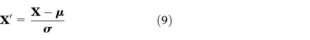
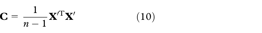
where μ and σ contain the mean and the standard deviation of each variable, respectively.

(2) The covariance matrix C of $X'$ is calculated as

C = \frac{1}{n - 1} X'^{T} X'

(10)

(3) By eigendecomposition,

C = V Λ V^{T}

(11)

where Λ is a diagonal matrix storing the eigenvalues λ₁,…, λ_m in a decreasing order, with the corresponding eigenvectors v ₁,…, v _m as the columns of V.

(4) The transformed matrix Y_pca is calculated by

Y_{pca} = X V_{q} Λ_{q}^{- 1 / 2}

(12)

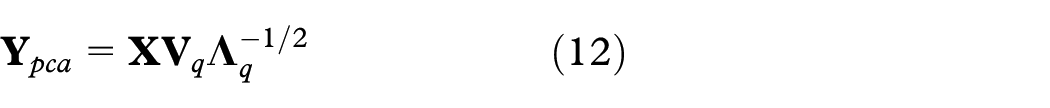
where $Λ_{q}$ and $V_{q}$ contain the q largest eigenvalues and the corresponding eigenvectors. For data visualization, q is commonly set to 2.

Bi-kernel t-SNE

In the testing procedure in kernel t-SNE, the difference between the outliers and inliers is submerged in Y. Outliers are not mapped well. To identify outliers, kernel functions are usually introduced to reveal the complex structure by mapping low-dimensional data to a high-dimensional space.²⁹ To this end, bi-kernel t-SNE is proposed. The Gaussian kernel function and PCA are introduced to reveal the difference and realize a correct mapping. Even though the feature kernel is near zero as the new sample is an outlier, the difference between the outlier and inliers can be revealed by PCA. Accordingly, the mapping from X to Y takes the following form:

\frac{k_{y} (y_{i}, y_{j})}{\sum_{l} k_{y} (y, y_{l})} = \sum_{k} a_{kj} \frac{k_{x} (x_{i}, x_{k})}{\sum_{l} k_{x} (x, x_{l})}

(13)

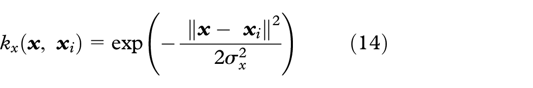
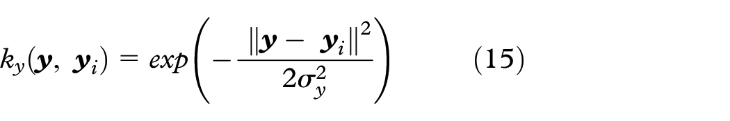
where k_x and k_y are the Gaussian kernels parameterized by the bandwidths σ_x and σ_y, respectively.

k_{x} (x, x_{i}) = \exp (- \frac{{‖ x - x_{i} ‖}^{2}}{2 σ_{x}^{2}})

(14)

k_{y} (y, y_{i}) = \exp (- \frac{{‖ y - y_{i} ‖}^{2}}{2 σ_{y}^{2}})

(15)

For each training and testing data, $\sum_{l} k_{y} (y, y_{l})$ and $\sum_{l} k_{x} (x, x_{l})$ are constants. Therefore, equation (13) can be derived to

k_{y} (y_{i}, y_{j}) = \sum_{k} w_{kj} \cdot k_{x} (x_{i}, x_{k})

(16)

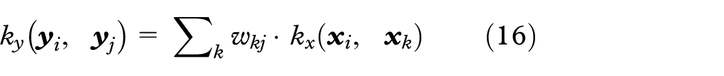
Assuming that W contains the parameters w_kj as its elements and K_x and K_y are the kernel matrices, we can rewrite equation (16) as

K_{y} = K_{x} W

(17)

We apply the least-squares method to solve the equation and obtain W.

W = (K_{x}^{T} K_{x})^{- 1} K_{x}^{T} K_{y}

(18)

Then PCA is applied to reduce the dimensionality of K_y to two for visualization.

Y = K_{y} V_{q} Λ_{q}^{- 1 / 2}

(19)

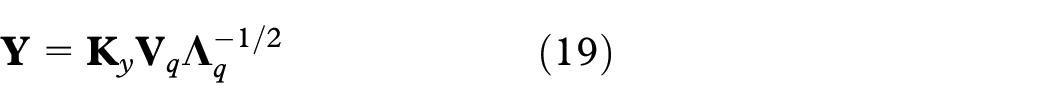
where $Λ_{q}$ and $V_{q}$ contain the q(q = 2) largest eigenvalues and the corresponding eigenvectors of K_y. Y is the required low-dimensional feature.

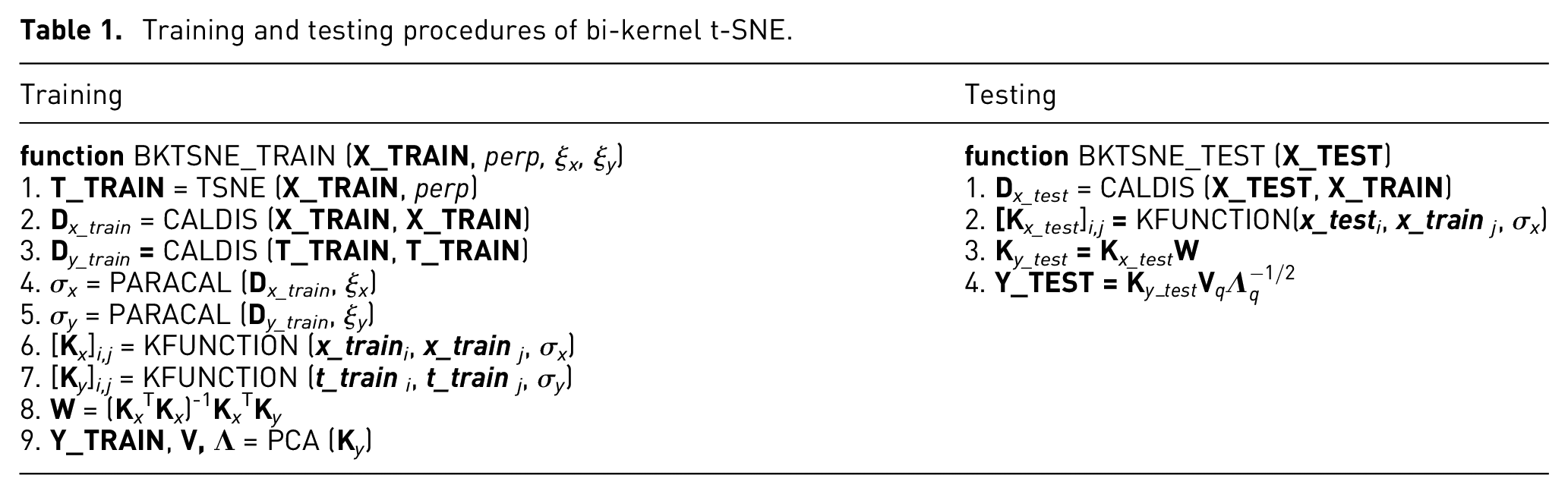
In bi-kernel t-SNE, the original t-SNE first maps X to obtain the training projection. Then, the kernel functions are used to obtain the kernel matrices K_x and K_y. The parameter matrix W is calculated using equation (18). PCA is applied to K_y to obtain the final feature Y. Once a new sample x _new arrives, the kernel vector k _x,new is calculated using x _new and training data X and multiplied with W to obtain k _y,new. The PCA testing procedure is performed on k _y,new to obtain the 2D projection y _new. Even through k _y,new is near zero when the new sample is an outlier, the difference between the fault and normal samples can be easily revealed by PCA, since the values of the elements in K_y are significantly greater than zero.

Table 1 summarizes the training and testing procedures of bi-kernel t-SNE. The matrices X_TRAIN and X_TEST contain the training and testing datasets, respectively. Y_TRAIN and Y_TEST are the obtained training and testing features, respectively. In TSNE, the original t-SNE algorithm is applied to X_TRAIN with a perplexity parameter perp. The pairwise Euclidean distances of all the samples in the given dataset are calculated in CALDIS. The KFUNCTION is used to calculate the kernel matrices with the parameter σ. In PARACAL, the parameters σ_x and σ_y are determined by specifying the lower bounds of the training kernels, that is, ξ_x and ξ_y. The basic idea of parameter selection is presented in Section 4.4. The code of our proposed method is publicly available at https://github.com/zhanghaily/bikernel-t-SNE.

Table 1.

Training and testing procedures of bi-kernel t-SNE.

Training	Testing
function BKTSNE_TRAIN (X_TRAIN, perp, ξ_x, ξ_y) 1. T_TRAIN = TSNE (X_TRAIN, perp) 2. D_{x_train}= CALDIS (X_TRAIN, X_TRAIN) 3. D_{y_train}= CALDIS (T_TRAIN, T_TRAIN) 4. σ_x = PARACAL (D_{x_train}, ξ_x) 5.σ_y = PARACAL (D_{y_train}, ξ_y) 6. [K_x]_i,j = KFUNCTION ( x_train _i, x_train _j, σ_x) 7. [K_y]_i,j = KFUNCTION ( t_train _i, t_train _j, σ_y) 8. W = (K_x^TK_x)^-1K_x^TK_y 9. Y_TRAIN, V, Λ = PCA (K_y)	function BKTSNE_TEST (X_TEST) 1. D_{x_test} = CALDIS (X_TEST, X_TRAIN) 2. [K_{x_test}]_i,j= KFUNCTION( x_test _i, x_train _j, σ_x) 3. K_{y_test}= K_{x_test}W 4. Y_TEST = $K_{y_test} V_{q} Λ_{q}^{- 1 / 2}$

Training

Testing

function BKTSNE_TRAIN (X_TRAIN, perp, ξ_x, ξ_y)
1. T_TRAIN = TSNE (X_TRAIN, perp)
2. D_{x_train}= CALDIS (X_TRAIN, X_TRAIN)
3. D_{y_train}= CALDIS (T_TRAIN, T_TRAIN)
4. σ_x = PARACAL (D_{x_train}, ξ_x)
5.σ_y = PARACAL (D_{y_train}, ξ_y)
6. [K_x]_i,j = KFUNCTION ( x_train _i, x_train _j, σ_x)
7. [K_y]_i,j = KFUNCTION ( t_train _i, t_train _j, σ_y)
8. W = (K_x^TK_x)^-1K_x^TK_y
9. Y_TRAIN, V, Λ = PCA (K_y)

function BKTSNE_TEST (X_TEST)
1. D_{x_test} = CALDIS (X_TEST, X_TRAIN)
2. [K_{x_test}]_i,j= KFUNCTION( x_test _i, x_train _j, σ_x)
3. K_{y_test}= K_{x_test}W
4. Y_TEST =

K_{y_test} V_{q} Λ_{q}^{- 1 / 2}

Parameter selection

Bi-kernel t-SNE has two parameters, that is, σ_x and σ_y, which are the bandwidths of the Gaussian kernel functions. The bandwidth determines the smoothness and divergence of the kernel function. Proper choice of the bandwidth will have a profound effect on the performance of the out-of-sample extension. According to the definition (equations (14) and (15)), the value of the Gaussian kernel decreases with increasing Euclidean distance and ranges between 0 and 1.

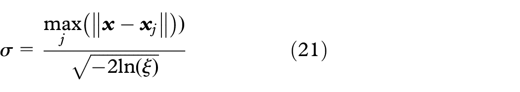
We present a practical way to determine the values of σ_x and σ_y in bi-kernel t-SNE. The main idea is that all elements in K_x and K_y should be within the range of representable numbers. The range should be within (0, 1] by definition. Bi-kernel t-SNE is expected to reveal the natural classes in training data and project outliers away from inliers. By specifying a lower bound ξ (0<ξ<1) for training data, range (0,1] is divided into two subranges, that is (0, ξ) and [ξ, 1]. The two subranges should be wide enough to clearly represent the known and unknown data structures, respectively. Specifically, the lower bound ξ of the Gaussian kernels should be neither too large nor too small.

For training data, the Gaussian kernel is equal to 1 when the two samples are the same, which is the upper bound of the range. The lower bound ξ can be derived as the kernel value of the farthest training data pair, which is

\exp (- \frac{max_{j} ({‖ x - x_{j} ‖}^{2})}{2 σ^{2}}) = ξ

(20)

where $\max (\cdot)$ means the maximum distance. Then by specifying ξ, we can get σ.

σ = \frac{max_{j} (‖ x - x_{j} ‖))}{\sqrt{- 2 \ln (ξ)}}

(21)

To get a robust kernel function, the farthest data pair is replaced by the median of the farthest l data pairs.

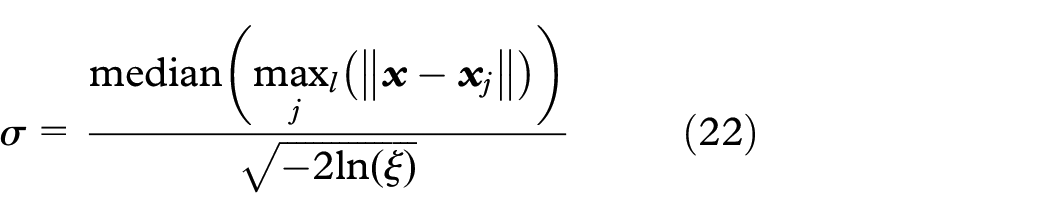
σ = \frac{median (\underset{j}{{max}_{l}} (‖ x - x_{j} ‖))}{\sqrt{- 2 \ln (ξ)}}

(22)

where $ma x_{l} (\cdot)$ means the greatest l distances, and $median (\cdot)$ calculates the median of them. l is equal to 10 in this study. Thus, the parameters, that is, σ_x and σ_y, can be determined by specifying ξ_x and ξ_y.

Evaluation measures

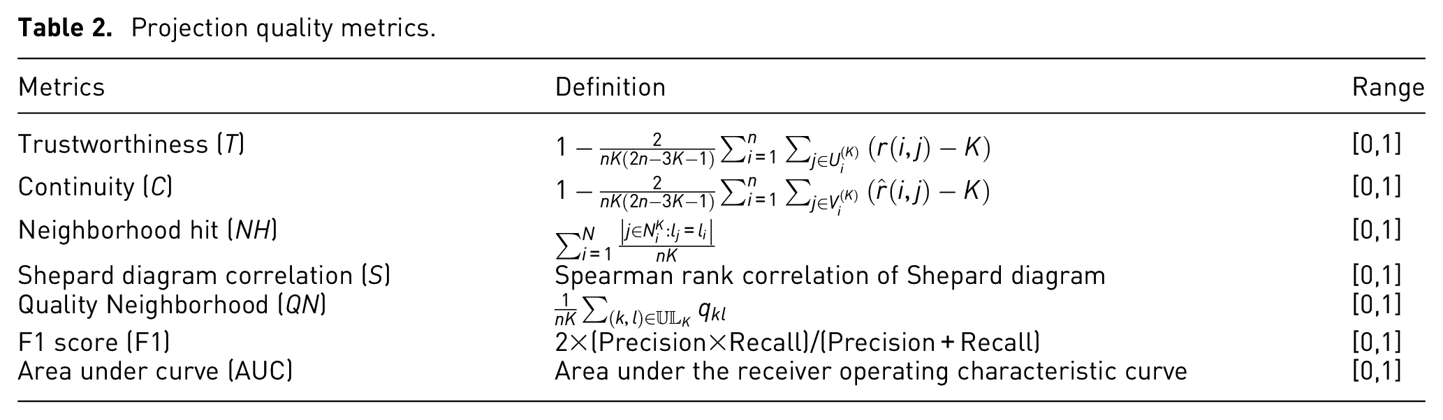
To evaluate the inlier and outlier projection ability of the proposed method, two sets of quality metrics are introduced for comparison with the state-of-the-art approaches. Trustworthiness, continuity, neighborhood hit, Shepard diagram correlation, and quality neighborhood are used to quantify the performance of bi-kernel t-SNE in inlier projection. F1 score and AUC are used for outlier projection quality evaluation. The definition of them are listed in Table 2.

Table 2.

Projection quality metrics.

Metrics	Definition	Range
Trustworthiness (T)	$1 - \frac{2}{nK (2 n - 3 K - 1)} \sum_{i = 1}^{n} \sum_{j \in U_{i}^{(K)}} (r (i, j) - K)$	[0,1]
Continuity (C)	$1 - \frac{2}{nK (2 n - 3 K - 1)} \sum_{i = 1}^{n} \sum_{j \in V_{i}^{(K)}} (\hat{r} (i, j) - K)$	[0,1]
Neighborhood hit (NH)	$\sum_{i = 1}^{N} \frac{\| j \in N_{i}^{K} : l_{j} = l_{i} \|}{nK}$	[0,1]
Shepard diagram correlation (S)	Spearman rank correlation of Shepard diagram	[0,1]
Quality Neighborhood (QN)	$\frac{1}{nK} \sum_{(k, l) \in U L_{K}} q_{kl}$	[0,1]
F1 score (F1)	2×(Precision×Recall)/(Precision+Recall)	[0,1]
Area under curve (AUC)	Area under the receiver operating characteristic curve	[0,1]

Quality metrics for inlier projection

Trustworthiness: T measures the proportion of points in X that are also close in Y. It tells how much one can trust that local patterns in a projection represent actual patterns in the data.²² In the definition (Table 2), $U_{i}^{(K)}$ is the set of points that are among the K nearest neighbors of y _i but not among the K nearest neighbors of x _i; and r(i, j) is the rank of y _j in the ordered set of nearest neighbors of y _i.

Continuity: C measures the proportion of points in Y that are also close in X.²² In the definition (Table 2), $V_{i}^{(K)}$ is the set of points that are among the K nearest neighbors of x _i but not among the K nearest neighbors of y _i; and $\hat{r} (i, j)$ is the rank of x _j in the ordered set of nearest neighbors of x _i.

Neighborhood hit: NH is the proportion of the K neighbors $N_{i}^{K}$ of y _i that have the same label l as x _i.²² It indicates if the projection is good for classification.

Shepard diagram correlation: S measures the quality of the Shepard diagram by computing its Spearman rank correlation. The Shepard diagram is a scatter plot of the pairwise (Euclidean) distances in Y versus the corresponding distances in X.²¹

Quality Neighborhood: QN measures the preservation of K neighborhoods. It tells how many neighbors stay the same.²⁴ $U L_{K}$ represents the upper-left blocks of the matrix, and q_kl is the element of the co-ranking matrix Q . The computing procedure of Q is detailed in literature.³⁰

All the quality metrics range in [0, 1] with 1 being the best. In this article, K is set to 10.

Quality metrics for outlier projection

The outliers should be detectable if they are mapped separated from the inliers. Here, the mean squared k-nearest neighbor distance D is used for outlier detection.³¹

D = \frac{1}{K} \sum_{i = 1, \dots, K} {‖ y - y_{i} ‖}^{2}

(23)

F1 score: F1 score is a weighted average of the precision and recall for the outliers.³² Precision is the ratio of the predicted true positive observations to the total number of actual positive observations. Recall is the ratio of the predicted true positives to the total number of observations predicted as positive. A threshold δ with a 95% confidence limit is used to identify whether a new testing point is positive or negative. The threshold is calculated using kernel density estimation.³³ If D > δ, it is an outlier. In this study, K is set to 10.

Area under curve: AUC is the area under the receiver operating characteristic (ROC) curve.³⁴ It reflects the performance of the model in separating inliers and outliers. The ROC curve is a graph of the true positive rate against the false positive rate at various threshold settings.

F1 score and AUC range in [0, 1], with 1 being the best.

Experiments

In this section (1) we discuss the parameter selection in bi-kernel t-SNE; (2) we test the ability of bi-kernel t-SNE in extending the t-SNE projection to inliers; (3) we test the performance of bi-kernel t-SNE in projecting outliers; (4) we measure the computational time needed for bi-kernel t-SNE with respect to varying number of samples. Both inliers and outliers are out-of-sample data. The inliers have the same labels as the training data. The outliers have different labels with the training data.

We use three out-of-sample extensions of t-SNE, that is, kernel t-SNE,¹⁹ LION t-SNE,²⁸ and DL t-SNE,²¹ and four parametric DR algorithms, that is, UMAP,³⁵ AE, PCA, and KPCA, as benchmark methods for comparison. The experiments were executed on a computer with Pytorch 1.3.1, Python 3.7.4, Windows 7, CPU: Intel Core i7-4710 2.5GHz, and RAM: 8GB. The quality metrics and computational time are averaged over 10 runs.

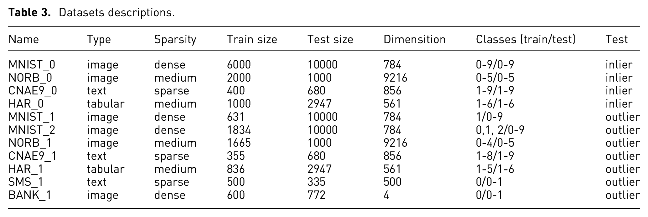
Based on data type, sparsity and dimensionality, we chose the following six datasets to conduct eleven experiments for inlier and outlier projection tests. The eleven subdatasets used in the experiments are descripted in Table 3. Among them, four subdatasets are used for inlier projection test and seven are used for outlier projection test.

The MNIST³⁶ dataset contains 60,000 handwritten digits images from 0 to 9. Each image has 28×28 pixels.

The NORB³⁷ dataset contains 48,600 different toys images under six different lighting conditions. The number of pixels of an image here is 96×96.

The CNAE9³⁸ dataset contains free text descriptions of Brazilian companies categorized into nine categories.

The Smartphone Dataset for Human Activity Recognition (HAR) dataset³⁹ is collected from 30 participants with six activities.

The SMS Spam Collection (SMS)⁴⁰ is a public set of SMS labeled messages collected for mobile phone spam research. There are 723 samples under class 0 and 112 samples under class 1.

The banknote authentication (BANK) data⁴¹ were extracted from images taken from genuine and forged banknote-like specimens. There are 762 observations under class 0 and 610 observations under class 1.

Table 3.

Datasets descriptions.

Name	Type	Sparsity	Train size	Test size	Dimensition	Classes (train/test)	Test
MNIST_0	image	dense	6000	10000	784	0-9/0-9	inlier
NORB_0	image	medium	2000	1000	9216	0-5/0-5	inlier
CNAE9_0	text	sparse	400	680	856	1-9/1-9	inlier
HAR_0	tabular	medium	1000	2947	561	1-6/1-6	inlier
MNIST_1	image	dense	631	10000	784	1/0-9	outlier
MNIST_2	image	dense	1834	10000	784	0,1, 2/0-9	outlier
NORB_1	image	medium	1665	1000	9216	0-4/0-5	outlier
CNAE9_1	text	sparse	355	680	856	1-8/1-9	outlier
HAR_1	tabular	medium	836	2947	561	1-5/1-6	outlier
SMS_1	text	sparse	500	335	500	0/0-1	outlier
BANK_1	image	dense	600	772	4	0/0-1	outlier

Parameter setting

We use NORB_1 and HAR_1 datasets to discuss the parameter setting in bi-kernel t-SNE. Different values (0.1, 0.2, 0.3, 0.4, 0.5, 0.6, 0.7, 0.8, and 0.9) were chosen for ξ_x and ξ_y to calculate the quality metrics. As all these metrics range over [0, 1], and we consider them equally important, the average of the seven quality metrics is used to evaluate the performance of different parameters. The results are shown in Figure 1. Darker color means better projection quality. For different datasets, the projection performances are slightly different. For NORB_1 dataset, the projection quality is better when ξ_x and ξ_y are greater. For HAR_1 dataset, it is better when ξ_x is smaller and ξ_y is greater. In general, better performance is obtained when 0.6≤ξ≤0.8. We set ξ_x and ξ_y to 0.7 in this study.

Figure 1.

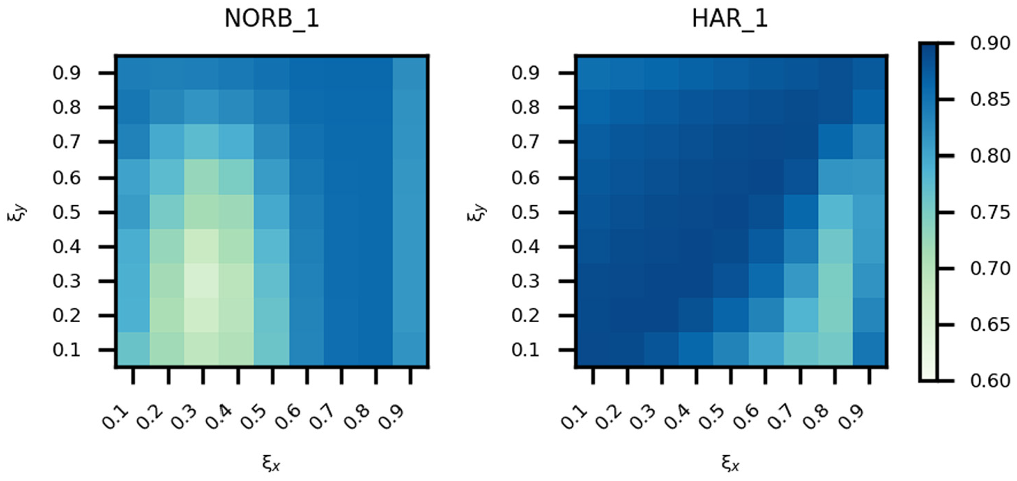
Projection performance of different parameters on NORB_1 and HAR_1 datasets.

Except for σ_x and σ_y, there are other parameters in bi-kernel t-SNE and other methods. The perplexity in all t-SNE-related methods is set to 40. The bandwidths in kernel t-SNE and KPCA are determined by the lower bound of the training kernel, which is the same as the way selecting σ_x and σ_y in bi-kernel t-SNE. DL t-SNE has three fully connected hidden layers, with 256, 512, and 256 units, respectively, followed by ReLU activation functions. It uses a two-element output layer and the sigmoid activation function to encode the 2D projection.²¹ The learning rate is set to 0.0001. The training epoch is 10. AE has one hidden layer with 16 neurons in the encode unit.²² The sigmoid function is used after each hidden layer. The number of neurons in the output layer is 2. The learning rate is set to 0.0001. The training epoch varies from 2 to 10 according to different sizes of the datasets.

Inlier projection test

Different classes in the training dataset are projected to separated regions in the 2D map by t-SNE. As an out-of-sample extension of t-SNE, bi-kernel t-SNE should be able to mimic the ground-truth projection and extend to inliers.

Figure 2 shows the ground-truth projections of bi-kernel t-SNE performing on four datasets, comparing to kernel t-SNE, LION t-SNE, DL t-SNE, UMAP, AE, PCA, and KPCA. In Figure 2, the training projection results of t-SNE-based methods are similar, which are better than other data visualization techniques. In particular, MNIST_0 and CNAE9_0 datasets can only be well projected by t-SNE-based methods and UMAP. Different clusters in NORB_0 and HAR_0 datasets are easily separated by all technologies, except that UMAP maps some samples that have the same label to separated regions.

Figure 2.

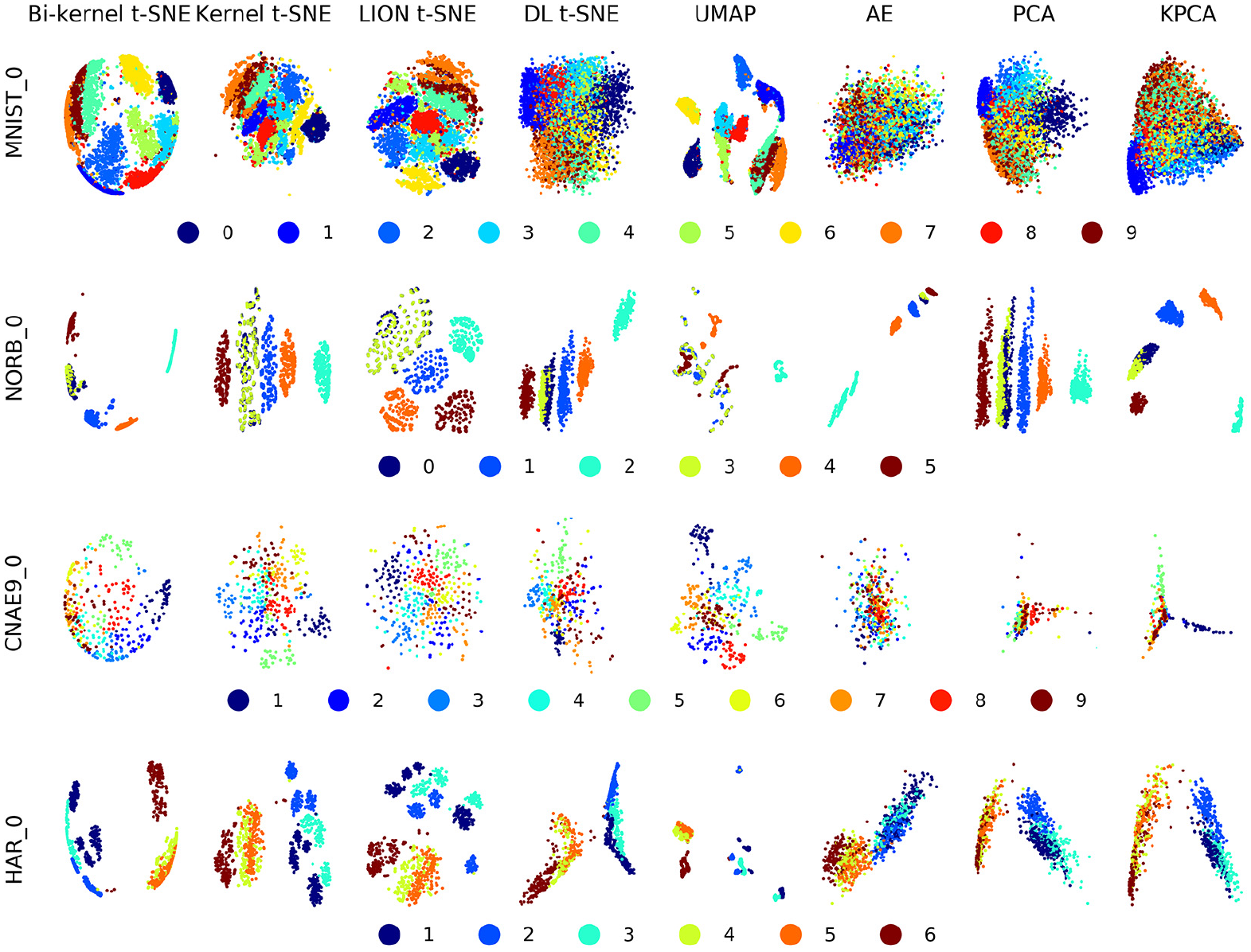
Training projection results of eight techniques on four datasets.

Figure 3 shows the inlier projections. Each color stays in the same area as it stays in Figure 2, which means that all methods can extend the projection to inliers. However, the testing projections can only be similar to or marginally worse than the training projections. The clusters in the testing projections mix more than in the training projections. In other words, if the ground-truth projection is worse than others, it is hardly possible that the testing projection will be better. To compare our proposed method with other state-of-the-art data visualization techniques, the quality metrics are calculated and shown in Figure 4. The quality metrics are slightly different for various algorithms on these four datasets. In general, t-SNE-related methods and UMAP obtain greater quality metrics on most datasets, compared with other state-of-the-art techniques. Bi-kernel t-SNE yields similar results to other t-SNE-based methods and UMAP, which indicates a well inlier projection ability.

Figure 3.

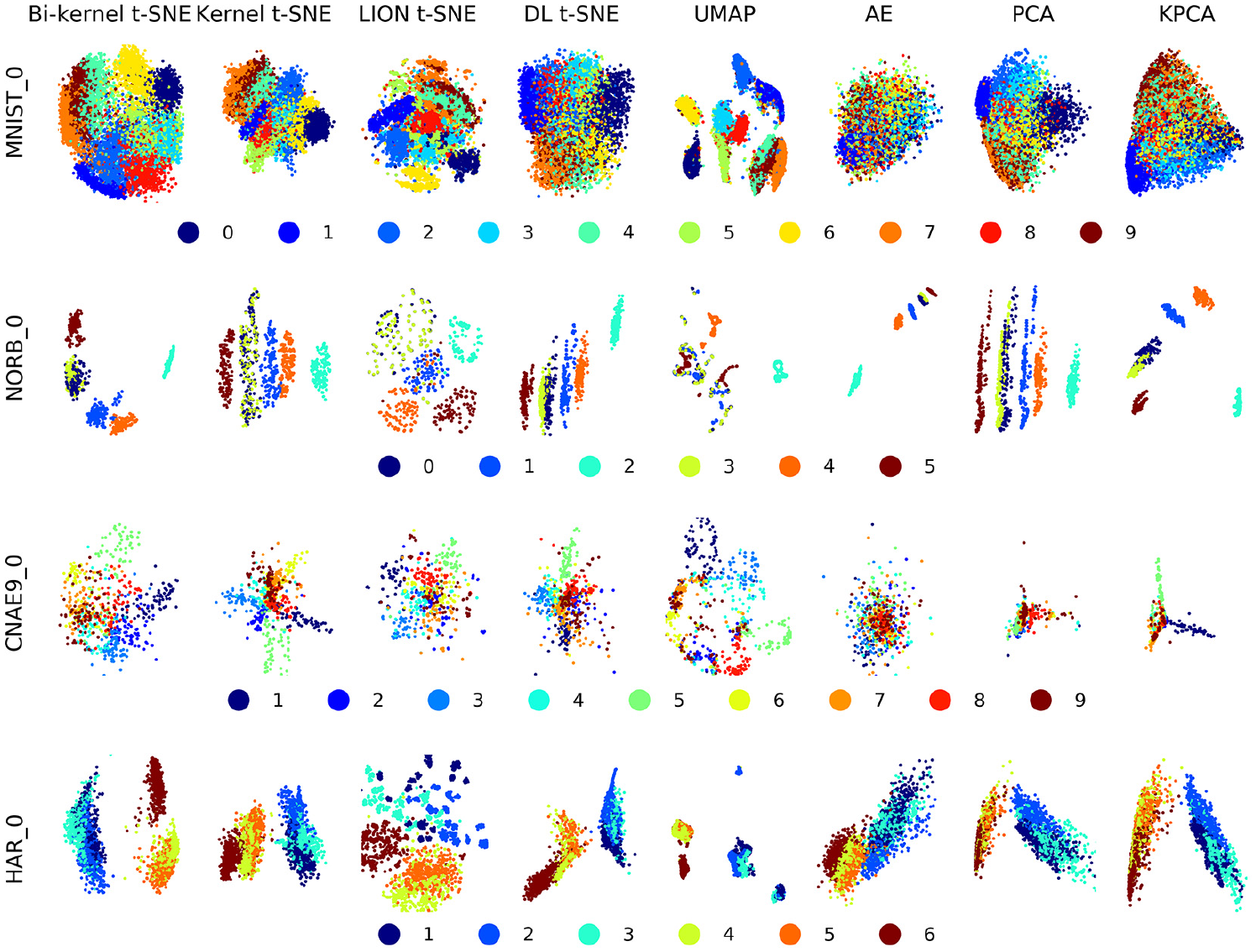
Testing inlier projection results of eight techniques on four datasets.

Figure 4.

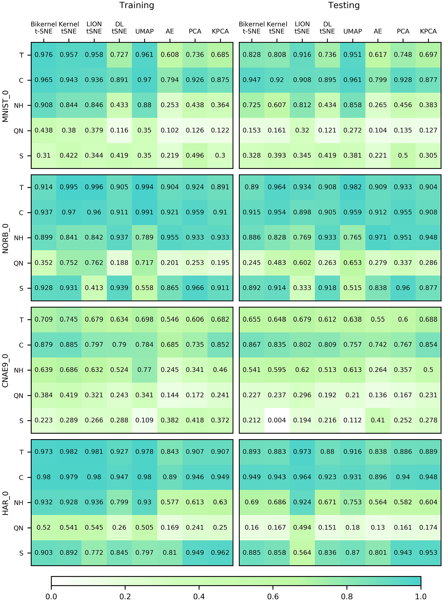
Inlier projection quality metrics comparison.

Outlier projection test

To evaluate the performance of bi-kernel t-SNE in outlier projection, seven experiments were conducted. In each experiment, the number of testing classes is more than that of training classes. Figure 5 shows the testing visualization results on seven datasets and Figure 6 shows the quality metrics, that is, F1 score and AUC.

Figure 5.

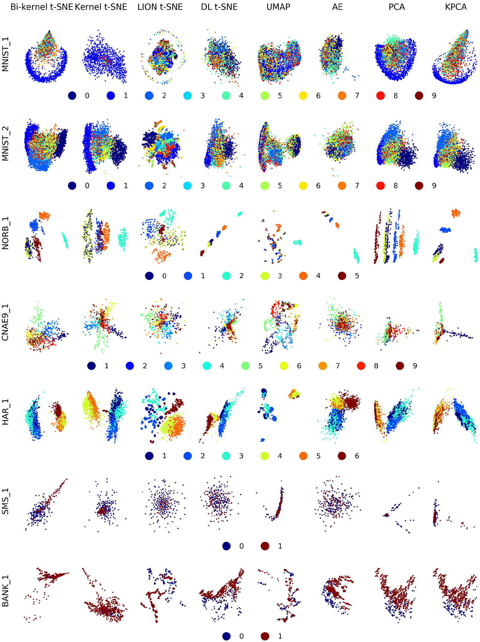
Outlier projection results of eight techniques on seven datasets.

Figure 6.

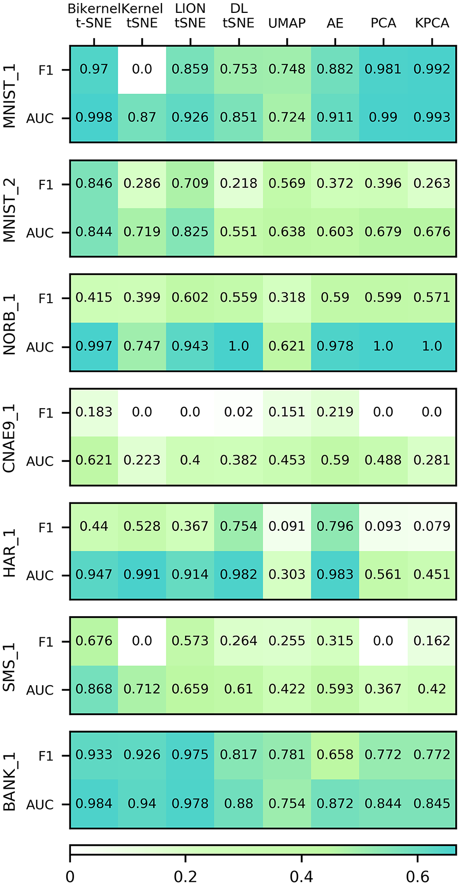
Outlier projection quality metrics comparison.

Firstly, we would like to discuss how bi-kernel t-SNE overcomes the aforementioned drawback of kernel t-SNE in outlier projection. Taking MNIST_1 dataset as an example, class 1 is used for model training and all the other nine classes are outliers. Outliers are usually far from the training set. The Gaussian kernel k_x, _new is extremely small or even near zero. The corresponding 2D projection of kernel t-SNE is near the origin. Since the 2D projections of the training data are also around the origin, the outliers mix with the inliers in the 2D map (row 1, column 2 in Figure 5). In bi-kernel t-SNE, k _y,new is near zero for an outlier, whereas the values of the training kernels are significantly greater than zero. The difference between the outliers and the inliers can easily be revealed by PCA. As a result, the outliers in MNIST_1 dataset are far away from the inliers by using bi-kernel t-SNE (row 1, column 1 in Figure 5). Correspondingly, the F1 score of kernel t-SNE are significantly lower than that of bi-kernel t-SNE for MNIST_1 dataset (Figure 6). Moreover, bi-kernel t-SNE obtains much better visualization results and much greater quality metrics on most datasets than kernel t-SNE.

Secondly, we compare bi-kernel t-SNE with other out-of-sample extensions of t-SNE and several state-of-the-art data projection methods. For MNIST_1 dataset, class 1 is used for model training and all the other nine classes are outliers. It can be seen that most methods can separate class 1 with other classes (row 1 in Figure 5). For MNIST_2 dataset, classes 0, 1, and 2 are used for training and the other seven classes are outliers. Only bi-kernel t-SNE and LION t-SNE can separate the outliers with the inliers (row 2 in Figure 5). F1 score and AUC of them are relatively greater than other methods (Figure 6). However, all methods cannot separate different classes in outliers. For the rest five datasets, samples from the last class are outliers. The outliers in NORB_1, HAR_1, and BANK_1 datasets are quite different from the inliers so that they can be correctly projected to separated regions by many methods (rows 3, 5, and 7 in Figure 5). However, for NORB_1 dataset, AUC of kernel t-SNE and UMAP is significantly lower than it of other methods (Figure 6). UMAP, PCA, and KPCA do not work well on HAR_1 dataset. For CNAE_9 and SMS_1 datasets, all data visualization techniques have considerable difficulty in separating the outliers with the inliers (rows 4 and 6 in Figure 5). Only our proposed method obtain greater F1 score and AUC on SMS_1 dataset (Figure 6).

Summarizing above, bi-kernel t-SNE and LION t-SNE are much better than others in separating outliers from inliers. Bi-kernel t-SNE yields better outlier projections than LION t-SNE on most datasets, especially on SMS_1 dataset.

Computational time comparison

Computational time measures the complexity of the algorithm, which is crucial to its applicability in large data projection. In this section, we compare the computational times of bi-kernel t-SNE, kernel t-SNE, LION t-SNE, and DL t-SNE. The running times of them are dominated by the original t-SNE and the respective out-of-sample mapping techniques.

The experiments were carried out on MNIST dataset. We used 500, 1000, 2000, 3000, 4000, 5000 and 6000 samples for training. Then we used the model trained by 2000 samples as the ground truth for testing. The number of testing samples also ranges from 500 to 6000. Figure 7 shows the results. The training procedure of LION t-SNE takes the least time since it is the same as the original t-SNE. Bi-kernel t-SNE is only a little slower than the other parametric extensions of t-SNE. In practice, one can train only once and extend the projection to bigger dataset. Hence, testing time is more important for a parametric projection technique. The testing procedures of bi-kernel t-SNE and kernel t-SNE take similar time, which is about one order of magnitude slower than DL t-SNE and two orders of magnitude faster than LION t-SNE. This is an important result, since LION t-SNE is the only out-of-sample extension of t-SNE that works well on outliers as we aware of. Only a little more training time and orders of magnitude less testing time, together with the projection quality, show that our proposed method is a competing alternative.

Figure 7.

Computational time comparison between bi-kernel t-SNE, kernel t-SNE, LION t-SNE, and DL t-SNE on MNIST dataset.

Discussion

Bi-kernel t-SNE enables out-of-sample extension for t-SNE, realizing convincing out-of-sample visualization results in linear time. With the bi-kernel mapping and PCA, our proposed method overcomes the drawback of kernel t-SNE in outlier projection. Specifically, bi-kernel t-SNE can extend the original t-SNE projection to inliers, achieving a similar inlier projection quality to kernel t-SNE, LION t-SNE, and DL t-SNE. For outlier projection, the performance of bi-kernel t-SNE is a little better than LION t-SNE and significantly better than other benchmark methods.

Only two parameters exist in bi-kernel t-SNE, except for the perplexity. They are the bandwidths of the Gaussian kernel functions and can be simply determined by specifying lower bounds for the training kernels. This is much easier than the parameter selection in pt-SNE. Moreover, there is no need to worry about overfitting in model training.

The computational time cost by the testing procedure of bi-kernel t-SNE is almost the same as kernel t-SNE and orders of magnitude less than LION t-SNE. Among the several out-of-sample extensions of t-SNE, LION t-SNE is the only one that works well on outliers as we aware of. Considering this, bi-kernel t-SNE is more applicable to visualize large data on a relatively low-performance equipment.

Bi-kernel t-SNE still has limitations in outlier visualization, which is also the well-known problem in machine learning. For example, when the outlier contains more than two classes, it is very possible that their 2D projections overlap with each other. A parametric data visualization method can only learn the data structure in the training data. For unseen data structures in outliers, however, most parametric DR algorithms have difficulty in revealing them. How to extend the original t-SNE projection to unrelated data and generate a well-separated outlier visualization is still a difficulty.

Conclusion

In this paper, a bi-kernel t-SNE is presented for out-of-sample data visualization, realizing convincing visualization results in linear time and overcoming the limitations of kernel t-SNE for outlier projection. The explicit mapping between the high-dimensional space and the low-dimensional space is approximated using the Gaussian kernel matrices of both input data and features. PCA is then introduced to reduce the dimensionality of the mapped kernel matrix and reveal the difference between the outliers and inliers. Two groups of comparative experiments conducted on the inlier and outlier projections demonstrate the ability of bi-kernel t-SNE.

This proposal opens the way for t-SNE toward outlier detection since the outliers and the inliers are well separated by bi-kernel t-SNE. Potential future work will expand on outlier online detection in other fields. Besides that, how to extend the ground-truth projection to unrelated data and generate a well-separated outlier visualization will be also considered in our future work.

Footnotes

Funding

The author(s) disclosed receipt of the following financial support for the research, authorship, and/or publication of this article: This work has been supported by National Natural Science Foundation of China (61803005, 61640312, and 61763037), Natural Science Foundation of Beijing Municipality (4192011 and 4172007), Key R & D project of Shandong Province (2018CXGC0608), China Scholarship Council, and the Beijing Municipal Commission of Education.

ORCID iD

Haili Zhang

References

Liu

. Challenges of feature selection for big data analytics. IEEE Intell Sys 2017; 32: 9–15.

Liu

Maljovec

Wang

, et al. Visualizing high-dimensional data: advances in the past decade. IEEE T Visual Comput Graph 2017; 32: 1249–1268.

Liang

Zhu

, et al. Review of classical dimensionality reduction and sample selection methods for large-scale data processing. Neurocomputing 2019; 328: 5–15.

Zhang

Cai

, et al. Face sketch aging via aging oriented principal component analysis. Pattern Recognit Lett 2018; 109: 65–71.

Zhao

Gao

. Fault-relevant Principal Component Analysis (FPCA) method for multivariate statistical modeling and process monitoring. Chemom Intell Lab Syst 2014; 133: 1–16.

Zhou

, et al. Randomized Kernel principal component analysis for modeling and monitoring of nonlinear industrial processes with massive data. Ind Eng Chem Res 2019; 58(24): 10410–10417.

Jain

Verma

Kumar

. Low cost localization using Nyström extended locally linear embedding. Pattern Recognit Lett 2018; 110: 30–35.

Wang

Wong

Lee

. Locally linear embedding with additive noise. Pattern Recognit Lett 2019; 123: 47–52.

Bengio

Paiement

Vincent

, et al. Out-of-sample extensions for LLE, Isomap, MDS, Eigenmaps, and spectral clustering. In: Proceedings of the sixteenth international conference on neural information processing systems, Vancouver and Whistler, Canada, 8–13 December 2003, pp.177–184. Cambridge: The MIT Press.

10.

Zhang

Qin

, et al. Semi-supervised local multi-manifold Isomap by linear embedding for feature extraction. Pattern Recognit 2018; 76: 662–678.

11.

Zhang

Peng

Dong

. A P-t-SNE and MMEMPM based quality-related process monitoring method for a variety of hot rolling processes. Control Eng Pract 2019; 89: 1–11.

12.

Ayesha

Hanif

Talib

. Overview and comparative study of dimensionality reduction techniques for high dimensional data. Inf Fusion 2020; 59: 44–58.

13.

Van Der Maaten

Hinton

. Visualizing data using t-SNE. JMLR 2008; 9: 2579–2605.

14.

Van Der Maaten

. Accelerating t-SNE using tree-based algorithms. JMLR 2014; 15: 1–21.

15.

Linderman

Rachh

Hoskins

, et al. Fast interpolation-based t-SNE for improved visualization of single-cell RNA-seq data. Nat Methods 2019; 16: 243–245.

16.

Tian

, et al. A feature extraction and visualization method for fault detection of marine diesel engines. Measurement 2017; 116: 429–437.

17.

Tang

Yan

. Neural network modeling relationship between inputs and state mapping plane obtained by FDA-t-SNE for visual industrial process monitoring. Appl Soft Comput J 2017; 60: 577–590.

18.

Liu

Yang

, et al. Generative principal component thermography for enhanced defect detection and analysis. IEEE Trans Instrum Meas 2020; 9456: 1–9.

19.

Gisbrecht

Schulz

Hammer

. Parametric nonlinear dimensionality reduction using kernel t-SNE. Neurocomputing 2015; 147: 71–82.

20.

Wang

Feng

, et al. Multi-view sparsity preserving projection for dimension reduction. Neurocomputing 2016; 216: 286–295.

21.

Espadoto

Hirata

Telea

. Deep learning multidimensional projections. Inf Vis 2020; 19: 247–269.

22.

Espadoto

Martins

Kerren

, et al. Towards a quantitative survey of dimension reduction techniques. IEEE Trans Visual Comput Graph 2021; 27(3): 2153–2173.

23.

Nonato

Aupetit

. Multidimensional projection for visual analytics: linking techniques with distortions, tasks, and layout enrichment. IEEE Trans Visual Comput Graph 2019; 25: 2650–2673.

24.

Lee

Verleysen

. Quality assessment of dimensionality reduction: rank-based criteria. Neurocomputing 2009; 72: 1431–1443.

25.

Van Der Maaten

. Learning a parametric embedding by preserving local structure. JMLR 2009; 5: 384–391.

26.

Zhu

Webb

Mao

, et al. A deep learning approach for process data visualization using t-distributed stochastic neighbor embedding. Ind Eng Chem Res 2019; 58: 9564–9575.

27.

Boytsov

Fouquet

Hartmann

, et al. Visualizing and exploring dynamic high-dimensional datasets with LION-tSNE. arXiv preprint arXiv: 1708.04983, 2017.

28.

Guo

Wang

. Weighted preliminary-summation-based principal component analysis for non-Gaussian processes. Control Eng Pract 2019; 87: 122–132.

29.

Liu

Guo

, et al. Kernel-based MinMax clustering methods with kernelization of the metric and auto-tuning hyper-parameters. Neurocomputing 2019; 359: 173–184.

30.

Lee

Verleysen

. Scale-independent quality criteria for dimensionality reduction. Pattern Recognit Lett 2010; 31: 2248–2257.

31.

Zhang

Zhao

Wang

, et al. Pseudo time-slice construction using a variable moving window k nearest neighbor rule for sequential uneven phase division and batch process monitoring. Ind Eng Chem Res 2017; 56: 728–740.

32.

Chai

Zhao

. Enhanced random forest with concurrent analysis of static and dynamic nodes for industrial fault classification. IEEE Trans Ind Informatics 2020; 16: 54–66.

33.

Zhang

Wang

, et al. Fault detection and diagnosis of chemical process using enhanced KECA. Chemom Intell Lab Sys 2017; 161: 61–69.

34.

Lin

Tang

Tianfield

, et al. A novel approach to reconstruction based saliency detection via convolutional neural network stacked with auto-encoder. Neurocomputing 2019; 349: 145–155.

35.

McInnes

Healy

Melville

. UMAP: uniform manifold approximation and projection for dimension reduction. arXiv preprint arXiv: 1802.03426, 2018.

36.

LeCun

Bottou

Bengio

, et al. Gradient-based learning applied to document recognition. Proc IEEE 1998; 86(11): 2278–2324.

37.

LeCun

Huang

Bottou

. Learning methods for generic object recognition with invariance to pose and lighting. In: Proceedings of the 2004 IEEE computer society conference on computer vision and pattern recognition 2004, Washington, DC, 27 June–2 July 2004, pp.97–104. New York: IEEE.

38.

Ciarelli

Oliveira

. Agglomeration and elimination of terms for dimensionality reduction. In: 2009 ninth international conference on intelligent systems design and applications, Pisa, 30 November–2 December 2009, pp.547–552. New York: IEEE.

39.

Reyes-Ortiz

Ghio

Parra

, et al. Human activity and motion disorder recognition: towards smarter interactive cognitive environments. In: 21th European symposium on artificial neural networks, Bruges, 24–26 April 2013, pp.403–412.

40.

Almeida

Hidalgo

Yamakami

. Contributions to the study of SMS spam filtering: new collection and results. In: Proceedings of the 2011 ACM symposium on document engineering, Mountain View, CA, 19–22 September 2011, pp.259–262. New York: ACM.

41.

Lohweg

Doerksen

. Banknote Authentication Data Set. UCI Machine Learning Repository. Irvine, CA: University of California, School of Information and Computer Science, 2012, https://archive.ics.uci.edu/ml/datasetsnknote+authentication