LCIP: Loss-controlled inverse projection of high-dimensional image data

Abstract

Projections, also known as dimensionality reduction methods, $P$ aim to map high-dimensional data to 2D scatterplots for visual exploration. Inverse projection methods $P^{- 1}$ aim to map this 2D space to the data space to support tasks such as data augmentation, classifier analysis, and data imputation. Current $P^{- 1}$ methods suffer from a fundamental limitation – they can only generate a fixed surface-like structure in data space, which poorly covers the richness of this space. We address this by a new method that ‘sweeps’ the data space by a surface that is not fixed but under user control. Our method works generically for any technique $P$ and dataset, is controlled by two intuitive user-set parameters, and is simple to implement. We demonstrate it by an extensive application involving image manipulation for style transfer.

Keywords

inverse projection disentanglement multidimensional data visualization adversarial training

Introduction

Multidimensional projections, also called dimensionality reduction (DR) methods, are established techniques for the visual exploration of high-dimensional data.^1–3 Many DR methods have been proposed in the past decades, such as PCA, t-SNE, and UMAP, to mention just a few.

Inverse projections aim to revert the mapping produced by a given projection. They aim to generate highly plausible, yet hypothetical, data items from any location in the embedding space created by projecting a given dataset. This enables applications such as data augmentation,^4,5 analyzing trained ML classification models by so-called decision maps.^6–8 pseudolabeling for creating training sets,⁵ morphing and data imputation,^9,10 and testing a classifier’s brittleness versus backdoor and data poisoning attacks.^8,11

Both direct and inverse projections suffer from significant information loss.¹² Direct projections cannot, in general, map data whose intrinsic dimensionality largely exceeds that of the 2D projection space while preserving data structure, that is, inter-point distances and neighborhoods.^3,13 Yet, users expect that inverse projections allow them to examine large parts of a data space starting from its 2D projection space. However, a recent study has shown that all current inverse projection techniques only generate fixed, surface-like, structures in the data space, so the coverage of inverse projections is limited to a small part of the data.¹⁴

In this work, we enable inverse projections to represent surface-like structures whose location in data space is not fixed (as produced by existing inverse projection techniques) but rather controllable by the user. Intuitively put, the user controls two parameters that allow the surface to move between a fixed position – given by the direct projection – and positions that get close to data samples deemed of interest by the user. As one changes the control parameters, the said surface literally ‘sweeps’ the data space. Even though, for a given set of control parameter values, we still produce a surface, its sweeping effect covers points which a single, fixed surface, computed by existing inverse projection techniques, could not reach. Specifically, for a sample $x$ projecting to $y = P (x)$ by a user-chosen technique $P$ , we find the information $z$ that is lost by $P$ and enable users to (interactively) control how to combine $y$ (information preserved by $P$ ) and $z$ (information lost by $P$ ) to compute our controllable inverse projection.

To realize this, we must answer three questions: (1) How to ensure $z$ is independent of $y$ (as we want to let $P$ compute $y$ and the user to control $z$ )? (2) How to compute $z$ for locations in the 2D space where no ground-truth sample $x$ projects? (3) How to control the structure created by the inverse projection, to enable users to explore large parts of the data space?

Our Loss-Controlled Inverse Projection (LCIP) answers these questions as follows: (1) We minimize mutual information to disentangle the $y$ and $z$ spaces. (2) We interpolate between $z$ values learned for known samples to fill in the ‘empty’ areas in a projection. (3) We allow users to interactively adapt $z$ to control the inverse projection’s shape.

To show our method’s abilities, we first study its disentanglement effect (section ‘Added value of disentanglement’) and next compare LCIP both visually and via quality metrics with 3 state-of-the-art inverse projections for 4 datasets and 2 direct projections (section ‘Comparison to other inverse projection methods’). Next, we show how LCIP’s interactive control creates higher-dimensional structures than surfaces, something existing methods cannot achieve (section ‘Controllability: Going beyond a fixed surface’). Finally, we show how our method can be used to support a style transfer application (section ‘User control of the inverse projection’). While our method can technically handle arbitrary high-dimensional data, we focus on image data which is easily interpretable – an important requirement for our technique where users aim to interactively control the structure created by the inverse projection (Figure 1).

Figure 1.

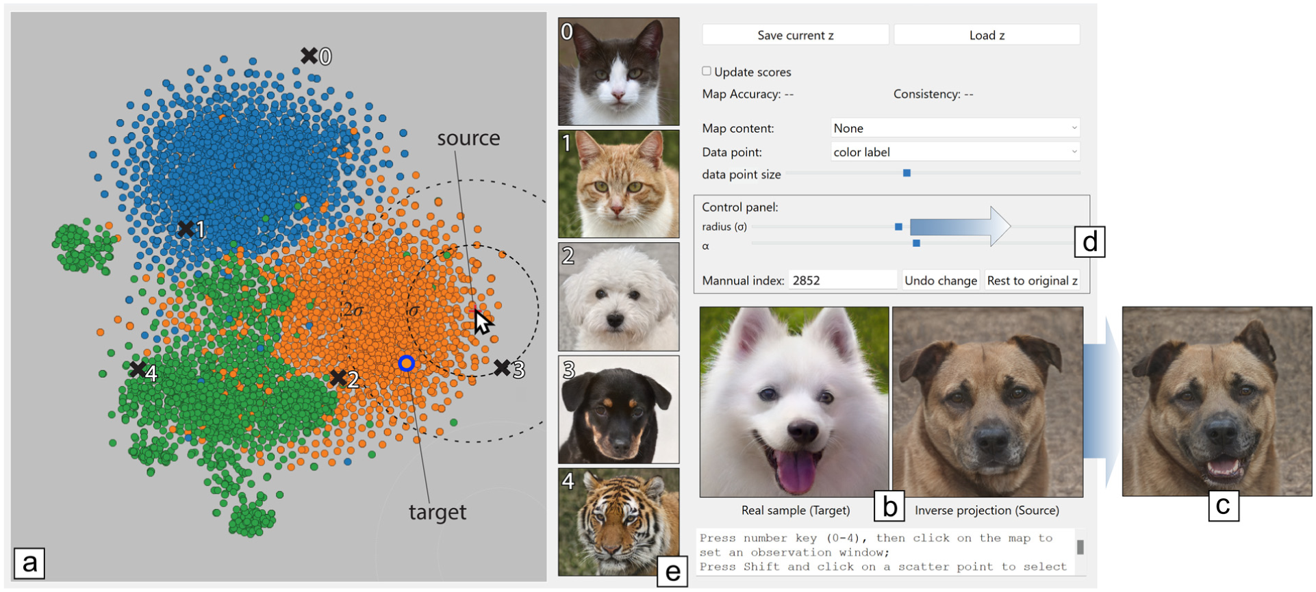
LCIP illustrated by a style transfer application. (1) Brush the projection (a) to find a frowning dog which we want to make smile (b, right). (2) Brush projection to find a target image with a smiling face (b, left). (3) Pulling a slider (d) changes the source towards the target, making the frowning dog smile without changing its identity, see result in (c). Adjusting the influence range $σ$ affects how images close to the source get changed towards the target – see circles centered at mouse location in (a). We select a few extra points in the projection – marked 0–4 in (a) – to inspect how LCIP behaves there. Point 3 is close to the source, so it is strongly influenced by the source’s change; points 0, 1, and 4 are far away from the source, so they are not affected.

Background and related work

Projections and inverse projections

Projection: Let $X = {x_{i}}$ , $x_{i} \in R^{n}$ , $1 \leq i \leq N$ , be an $n$ -dimensional dataset. A projection

P (X) = {y_{i}} \subset R^{q}

(1)

maps each $x_{i} \in X$ to a $y_{i} \in R^{q}$ , where $q << n$ . For visualization goals as in this work, we typically set $q = 2$ . Projection techniques, such as PCA, t-SNE¹⁵ and UMAP,¹⁶ are covered by extensive surveys.^3,13 We further denote any point in the projection space $R^{2}$ by $p$ .

Inverse projection: An inverse projection, also called backprojection or unprojection, is a function

P^{- 1} : R^{q} \to R^{n}

(2)

that aims to reverse the effect of a given $P$ . We next denote by $q$ points in the data space obtained by applying the inverse to some 2D point $p$ , that is, $q = P^{- 1} (p) .$ For a dataset $X$ and its projection $Y = P (X)$ , $P^{- 1}$ is typically computed by minimizing errors of the form $∥ P^{- 1} (P (x_{i})) - x_{i} ∥$ over $X$ . Crucially for applications, once $P^{- 1}$ is defined based on $X$ and $Y$ , one can use it to infer data values for any $p \in R^{2}$ , including so-called ‘gap areas’ $R^{2} ∖ Y$ between points in $Y$ .

Unlike direct projections, only a few inverse projection methods exist. iLAMP⁹ builds local affine mappings that revert the LAMP direct projection.¹⁷ To address the lack of continuity and global mapping in iLAMP, a method using Radial Basis Functions (RBFs) was next proposed,¹⁸ UMAP¹⁶ builds both a direct and inverse projection based on preserving the data structure’s topology from $R^{n}$ to $R^{q}$ . DeepView⁸ enhanced UMAP with a classifier to produce a discriminative projection and used a modified UMAP for inverse projection. Self-Supervised Network Projection (SSNP)¹⁹ enhanced standard autoencoders²⁰ with self-supervision using pseudolabels to create both direct and inverse projections. Blumberg et al.²¹ proposed a method to invert multidimensional scaling (MDS) that works well for $q < 10$ .^22,23 Finally, NNinv^10,24 used supervised deep learning to invert any projection $P (X)$ in a generic way, a method recently extended to autoencoders.²⁵

Inverse projection applications: Inverse projections allow performing dynamic imputation to explore a high-dimensional data space using its projection¹⁰; Amorim et al.¹⁸ morphed between facial expressions using RBF inverse projections. Inverse projections enable creating so-called decision maps. Such maps provide insights into a trained classification model’s behavior^7,8; allow pseudolabeling samples to create rich training sets⁵; and support explorations such as studying a model’s brittleness against data attacks.¹¹ In all such applications, inverse projections are a key element of interactive visualization: In Amorim et al.¹⁸, users interactively sweep the projection space to create 3D models that morph between those present in a given set. In decision map applications, users interactively brush the decision map (created using inverse projections) to find which types of samples project for example, in areas close to decision boundaries or in other zones where misclassifications can occur. An extension of this scenario allows users to locate wrongly-classified zones in decision maps and interactively select samples falling in such areas to improve classification performance.⁵ In our work, we extend this interactivity by allowing users to actually determine the shape of the inverse projection.

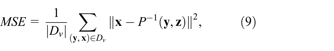
Quality of inverse projections: Quality of inverse projections can be measured by the MSE $∥ P^{- 1} (P (x)) - x ∥$ , for points $x \in X$ ; for so-called gap points, where inverse projections are actually useful, we do not have ground truth to test against. Previous work^10,11,18,26 shows that smooth inverse projections are preferred as they ensure that small changes in 2D space (e.g. when the user drags a 2D point to unproject) yield small changes in data space. Gradient maps¹⁰ gauge this smoothness by computing the norm of the gradient of $P^{- 1}$ . Additional metrics capture the quality of decision maps^11,26– these go however beyond evaluating inverse projections. We will use both MSE and gradient maps to evaluate our proposal.

Surface limitation of inverse projections: Recent work¹⁴ showed that all existing inverse projections map the 2D space to a fixed structure embedded in data space that is surface-like, that is, has intrinsic dimensionality close to two.²⁷ While not unexpected, given that a $P^{- 1}$ aims to smoothly map $R^{2}$ to $R^{n}$ , this means that inverse projections only cover a very limited subspace of $R^{n}$ . How this subspace is constructed is completely non-transparent to, and not controllable by, users. The above imply serious limitations for inverse projection applications. Using inverse projections for data augmentation will lack diversity. One cannot be sure that a decision map truly depicts a classifier’s behavior when it shows only a small part of the data space – more exactly, the cuts of the true decision zones by the surface structure created by $P^{- 1}$ .¹⁴ How to explore the data space outside this surface structure and how to control this exploration, are two challenges not answered by existing methods. In our work, we enable users to interactively control how such surface structures sweep the data space via simple visual controls.

Information loss: Both direct and inverse projections incur information loss. For direct projections, if the data $X$ do not land on or close to a manifold, constructing a mapping $P (X)$ that fully preserves data structure is hard.¹² Inverse projection limitations are stronger – these always create a surface-like structure as discussed above. If we consider the project-unproject cycle, information loss always occurs.

Inverse projections are structurally similar to data reconstruction or data generation tasks that create high-dimensional data from low-dimensional representations. The ( $P$ , $P^{- 1}$ ) cycle can be seen as an encoder-decoder structure, where the bottleneck is the 2D latent space. The dimensionality of this space is a critical factor for the quality of reconstruction and generation.^28–30 Inspired by these observations, we aim to break the limitations imposed by our bottleneck – the visual space – by retrieving information lost during $P$ and using it to drive the construction of $P^{- 1}$ under user control. This will enable our $P^{- 1}$ to span structures with higher intrinsic dimensionality than two, and also control where these are placed in data space.

Disentangled representations and adversarial training

As stated in section ‘Introduction’, our first goal is to find the information $z$ lost during projection independent of the projection $y$ . Independence is often relaxed to minimizing mutual information or separating complementary factors.³¹ When achieved, this improves interpretability, reduces potential bias, and enhances generalization. For example, in handwriting recognition, separating text content $y$ (what an actual letter is) from its style $z$ (how the letter is written) helps model generalization. In speech processing, one aims to separate speech content $y$ from speaker’s identity $z$ .³²

Minimizing mutual information between two latent representations, also called learning disentangled representations, can be done via adversarial training.^32–36 Adversarial training, first used by generative adversarial networks (GANs) for image generation,³⁷ creates high-dimensional realistic samples from low-dimensional latent codes. GANs jointly train a generator $G$ and a discriminator $Dis$ ; $G$ aims to create samples indistinguishable from real samples; $Dis$ tries to distinguish real from generated samples. Adversarial training has been extended to robust machine learning, domain adaptation, and disentangled representation learning. While diffusion models are now more popular for image generation, GANs are significantly more efficient.³⁸ For example, DragGAN,³⁸ an interactive image manipulation method, uses the StyleGAN2 architecture.³⁹

Directly projecting high-dimensional datasets such as high-resolution images is challenging. In such cases, one typically models the data in the latent space of a pre-trained classifier such as InceptionV3 or VGG16.^5,40 As we focus on inverse projection, we will retrieve images from the latent space of a generative model designed for this purpose, namely StyleGAN2. In detail: Let $w \in W$ be the latent code that StyleGAN2 uses to generate images. Codes $w$ can be obtained by inverting StyleGAN2 pre-trained on the same dataset.³⁹ For a given $w$ , the corresponding image is then given by $G (w)$ . Adversarial training connects to our work in two ways: (1) We use it to enforce disentanglement between the information $z$ and the projection $y$ during the training of our inverse projection. (2) We use the $W$ space of an image dataset to ease the projection process.

Design of loss-controlled inverse projection

Inverse projection deep learning network architecture

We implement our inverse projection using neural networks. Consider a dataset $X$ and its projection $Y = P (X)$ computed by any user-chosen projection technique $P$ . Our network has two key parts: an encoder $Enc$ that computes the information in $X$ lost by $P$ ; and a decoder $Dec$ which is also our inverse projection $P^{- 1}$ . $Enc$ reads the data $X$ and outputs a latent code $Z = Enc (X) = {z_{i}}$ . $Dec$ reads the concatenation $Y \oplus Z$ and outputs the inversely projected data $X^{'} = Dec (Y, Z)$ (Figure 2(a)). We also need to ensure that $Z$ is not related to $Y$ (see section ‘Disentangled representations and adversarial training’). We do this by a third discriminator network $Dis$ ; this network reads $Z$ and outputs $Y^{'} = Dis (Z)$ and is adversarially trained to minimize the error between $Y$ and $Y^{'}$ . $Enc$ and $Dec$ are jointly trained to (i) minimize the reconstruction error between $X$ and $X^{'}$ , and (ii) maximize the difference between $Y$ and $Y^{'}$ .

Figure 2.

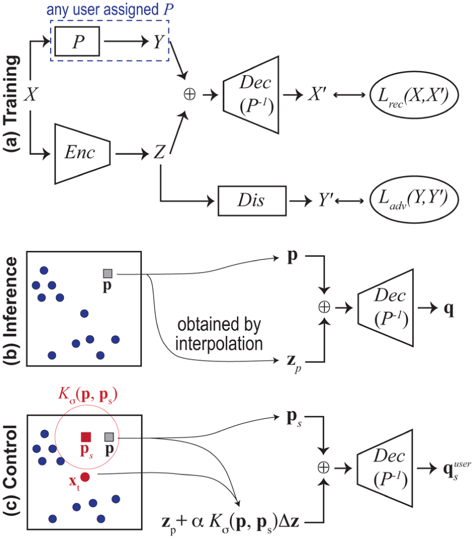
LCIP workflow. ⊕ denotes concatenation. (a) Training $Dis$ and $Dec$ . $P$ is a user-selected DR method that projects $X$ to $Y$ . $Enc$ encodes $X$ into $Z$ . $Dis$ uses $Z$ to predict $Y$ . $Dec$ ( $P^{- 1}$ ) uses $Y$ and $Z$ to reconstruct $X$ . The adversarial network $Dis$ enforces disentanglement (section ‘Inverse projection deep learning network architecture’). (b) Inversely projecting a 2D point $p$ to data sample $q$ (section ‘Computing $z$ for the entire projection space’). (c) Users can refine the inverse projection by maneuvering the controls marked in red: a source point $p_{s}$ , a target point $x_{t}$ , a pull factor $α$ , and a kernel radius $σ$ (section ‘Controlling the inverse projection’).

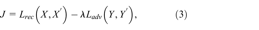
Let $θ_{Enc}$ , $θ_{Dec}$ , $θ_{Dis}$ be the weight and bias parameters of $Enc$ , $Dec$ , and $Dis$ , respectively. Let $L_{adv} (Y, Y^{'})$ be the reconstruction loss between $Y$ and $Y^{'}$ , and $L_{rec} (X, X^{'})$ the reconstruction loss between $X$ and $X^{'}$ . When optimizing $θ_{Dis}$ , we minimize $L_{adv}$ , so $Dis$ learns to predict $Y$ from $Z$ . The cost function $J$ for optimizing $Enc$ and $Dec$ is given by

J = L_{rec} (X, X^{'}) - λ L_{adv} (Y, Y^{'}),

(3)

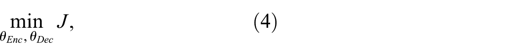
where $λ > 0$ is a hyperparameter that balances reconstruction versus adversarial loss, with the target of the optimization being

\min_{θ_{Enc}, θ_{Dec}} J,

(4)

that is, we minimize $L_{rec}$ and maximize $L_{adv}$ while keeping $θ_{Dis}$ fixed. Once trained, $Enc$ infers $Z$ from $X$ and $Dec$ next inversely projects $Y \oplus Z$ to $X'$ .

Implementation: We use fully-connected networks for $Enc$ , $Dec$ , and $Dis$ . $Enc$ has 3 hidden layers (sizes 512, 256, and 128). $Dec$ has 4 hidden layers (sizes 128, 256, 512, and 1024). Each hidden layer of $Enc$ and $Dec$ is followed by a ReLU activation function. The final layer of $Dec$ is followed by a sigmoid activation function. $Dis$ has 2 hidden layers, each with a size of 128. Each hidden layer is followed by batch normalization and a ReLU activation function. The dimension of $Z$ is set to 16 – a value we empirically found to be sufficient to capture the information loss of all studied $P$ techniques. We use these settings consistently for all tested datasets.

We use mean squared error (MSE) for both $L_{rec}$ and $L_{adv}$ (equation (3)). For $λ$ (equation (3)), we ran a grid search over the range $[0.005, 4]$ , and found that $λ \in [0.01, 0.1]$ gives good results for all tested datasets. We train all networks using the Adam optimizer with a learning rate of $0.001$ . While training $Dis$ , we have noticed that the adversarial training requires more steps to stabilize, since it learns from a changing input. Hence, at each iteration, we update $Dis$ 5 times, then update $Enc$ and $Dec$ once. Our work is implemented using PyTorch⁴¹ with PySide6 (Qt) for the GUI, and is publicly available.⁴²

Computing $z$ for the entire projection space

To apply our inverse projection (section ‘Inverse projection deep learning network architecture’) at a 2D projection point $y_{i}$ , we need the latent code $z_{i} = Enc (x_{i})$ computed from the sample $x_{i} \in X$ that projects to $y_{i}$ . To apply our method to any 2D point $p$ , we need to estimate $z_{p}$ at that location. We do this by interpolating the $z_{i}$ values of the samples $X$ (see Figure 2(b)). We tested two methods: weighted k-NN ( $k = 10$ neighbors) and smoothed RBF with a parameter-free thin plate spline kernel. RBF gives a smooth surface, while weighted k-NN is slightly faster. We discuss both interpolation methods in section ‘Comparison to other inverse projection methods’.

Having now the latent code $z_{p}$ for any $p \in R^{2}$ , we can inversely project $p$ to the data space (Figure 2(b)) as

q = P^{- 1} (p) = Dec (p, z_{p})

(5)

Controlling the inverse projection

To allow users to effectively control the shape of the inverse projection in data space, two questions arise: (1) How to do this easily, that is, by changing a small number of intuitive parameters in a direct, visual way; and (2) How to make our $P^{- 1}$ cover zones in data space where plausible samples exist, so that $P^{- 1}$ is useful for real-world applications.

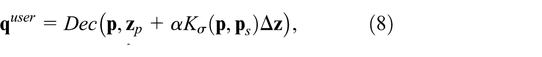
We solve both problems by the pipeline shown in Figure 2(c), which we explain next (see also Figure 3). Let $x_{t} \in X$ , called a target sample, be a data point that we want to make our inverse projection go close to. Users can discover such points by brushing the projection with a tooltip to see the values $x_{t}$ (Figure 3, green point). The user next selects a 2D source point $p_{s}$ and manipulates it to control $P^{- 1}$ (Figure 3, yellow point). We then ‘pull’ the inverse projection $P^{- 1} (p_{s})$ of $p_{s}$ towards $x_{t}$ by adjusting $z_{p_{s}}$ (initially computed by interpolation as described in section ‘Computing z for the entire projection space’) – see the red arrow in Figure 3. To achieve this pull, we first compute the difference

\begin{matrix} \begin{matrix} Δ z & = z_{t} - z_{p_{s}} = Enc (x_{t}) - z_{p_{s}} \end{matrix} \end{matrix}

(6)

Intuitively, $Δ z$ tells how much the latent codes of the source and target differ, that is, what we need to change in the source’s inverse projection to make it become the target. With $Δ z$ , we compute the user-controlled inverse projection of $p_{s}$ as

q_{s}^{user} = Dec (p_{s}, z_{p_{s}} + α Δ z),

(7)

where $α \in R$ is a factor giving the pull magnitude (Figure 3, light blue point). Yet, this adjustment only changes $P^{- 1}$ at the single location $q_{s}^{user}$ . 2D points close to $p_{s}$ will not be affected by this pull, as their inverse projections still follow equation (5). The inverse projection will exhibit a discontinuity or lack of smoothness around $q_{s}^{user}$ , which is undesired (section ‘Projections and inverse projections’). We could get smoothness by applying $Δ z$ to all such 2D points. However, this changes the inverse projection globally– the source $p_{s}$ will equally influence all inversely-projected points, no matter how far these are from $p_{s}$ . We jointly achieve smoothness and local control by weighing the adjustment based on distances in the projection space to the source $p_{s}$ . That is, after adjusting the inverse projection at $p_{s}$ (equation (7)), we replace equation (5) by

q^{user} = Dec (p, z_{p} + α K_{σ} (p, p_{s}) Δ z),

(8)

where $K_{σ} (p, p_{s}) = e^{- \frac{∥ p - p_{s} ∥^{2}}{2 σ^{2}}}$ is a Gaussian centered at $p_{s}$ and $σ$ controls the source’s influence. Larger $σ$ values make control more global and yield smoother inverse projections; smaller values work oppositely. When $p$ is close to the source $p_{s}$ (Figure 3 purple point), its inverse projection gets pulled towards the target $x_{t}$ – see light-blue bump on the surface in Figure 3. When $p$ is far from $p_{s}$ (Figure 3 orange point), its inverse projection stays on the surface given by equation (5). Figure 1 shows this control mechanism in action for a simple style transfer application. Here, the dataset $X$ contains images of various animal faces. The user selects the source $p$ by picking a location in the projection – not necessarily an actual projected sample. The image $q$ for this point is computed by the inverse projection – see the sad-looking dog in Figure 1(b), right. Next, the user selects a target sample $x_{t}$ – see the happy-looking dog in Figure 1(b), left. Pulling a slider changes $α$ and morphs the source towards the target. The user can see how far/strong the effect of changing the source propagates over the projection by selecting other images (Figure 1(e)) and assessing their changes during source manipulation.

Figure 3.

Controlling the inverse projection. User parameters are marked in red.

Evaluation

We evaluate our inverse projection method on several datasets and projection techniques. We first study the effect of disentanglement both qualitatively and quantitatively and show that our latent codes $z$ are indeed independent of the projected information $y$ (section ‘Added value of disentanglement’). Then, we show that our inverse projection (without interactive control) reaches similar quality to existing inverse projection methods (section ‘Comparison to other inverse projection methods’). Finally, we show that our interactive control breaks the surface-like limitation discussed in section ‘Controllability: Going beyond a fixed surface’.

For $P$ we use t-SNE and UMAP, known for their high quality¹³ and used in other inverse-projection studies.^8,10,24,26 Given their high quality, measured for example, by trustworthiness, continuity, and other projection quality metrics on a range of datasets and hyperparameter settings (see Espadoto et al.¹³ for details), this means that the vector $z$ will capture, globally speaking, the information present in the high-dimensional data $X$ which the projection was unable to capture due to the intrinsic dimensionality of $X$ exceeding two and not ‘spurious’ errors caused by the projection algorithm itself.

We use the following datasets:

MNIST: 70K samples of handwritten digits (0–9), each a $28^{2}$ grayscale image flattened to a 784-size vector.⁴³

Fashion-MNIST: 70K samples of 10 fashion categories (e.g. T-shirts, trousers, dresses), each a $28^{2}$ grayscale image flattened to a 784-size vector.⁴⁴

HAR: 10K samples of smartphone accelerometer and gyroscope data capturing six human activities (walk, walk upstairs, walk downstairs, sit, stand, lay).⁴⁵

$W$ of AFHQv2: AFHQv2 has 15K color images of animal faces in 3 classes: dogs, cats, wild animals.⁴⁶ Its $W$ is a $R^{512}$ latent space used by StyleGAN2 models³⁹ to generate images (section ‘Disentangled representations and adversarial training’). For ease of exposition, we next show the generated images $G (w)$ instead of the raw codes $w$ .

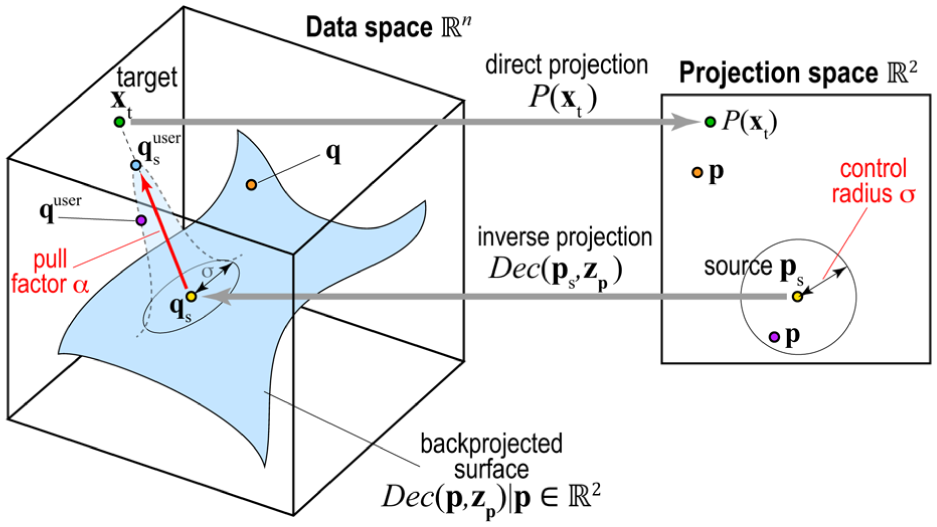
For a dataset $X = {x_{i}}$ and its projection $Y = {y_{i}}$ , $y_{i} = P (x_{i})$ , we form the pairedset $D = {(X, Y)}$ , and split it into training $D_{T} = {(X_{T}, Y_{T})}$ and test $D_{v} = {(X_{v}, Y_{v})}$ subsets. Table 1 summarizes the above, including the dataset-specific choice of the hyperparameter $λ$ (equation (3)).

Table 1.

Datasets used in our evaluation with dimensionality $n$ , sample count $| X |$ , training and testing set sizes $| D_{T} |$ and $| D_{v} |$ , and values of hyperparameter $λ$ (equation (3)).

Dataset	$n$	$\| D_{T} \|$	$\| D_{v} \|$	$\| X \|$	$λ$
MNIST	784	5000	5000	70,000	0.1
Fashion-MNIST	784	5000	5000	70,000	0.1
HAR	561	5000	5000	10,299	0.05
$W$ of AFHQv2	512	5000	5000	14,336	0.01

Added value of disentanglement

To show the added value of the disentanglement, we compare our results using the loss in equation (3); (called next WithDis) with the same network trained without $L_{adv}$ (called next NoDis).

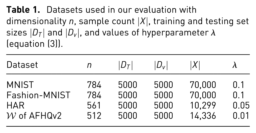
Quantitative evaluation: We measure disentanglement by how well $z$ predicts $y$ . Poor predictions mean better disentanglement, that is, more independent $z$ and $y$ .^31,35,47 We measure this by training a post hoc regression model to predict $Y_{T}$ from $Z_{T} = Enc (X_{T})$ . This model is a neural network with one hidden layer (100 units) followed by ReLU activation, trained for 200 epochs using the Adam optimizer. We measure $R^{2}$ and $MSE$ on a hold-out test set. We expect that WithDis should yield low $R^{2}$ and high $MSE$ – that is, $z$ and $y$ are independent and/or different. Conversely, we expect that NoDis should yield high $R^{2}$ and low $MSE$ – that is, $z$ and $y$ are correlated and/or similar. Table 2 shows that $MSE$ and $R^{2}$ for WithDis and NoDis indeed match the expectations, thus confirming our claimed disentanglement.

Table 2.

Measuring disentanglement: How well can $z$ predict $y$ ?

Dataset	$P$	WithDis		NoDis
Dataset	$P$	$MSE$	$R^{2}$	$MSE$	$R^{2}$
MNIST	UMAP	17.1	0.032	1.7	0.900
MNIST	t-SNE	1497.5	0.011	161.9	0.892
Fashion-MNIST	UMAP	19.9	0.201	0.7	0.968
Fashion-MNIST	t-SNE	1284.4	0.096	79.4	0.944
HAR	UMAP	48.8	0.098	6.9	0.862
HAR	t-SNE	1337.8	0.170	152.7	0.892
$W$ of AFHQv2	UMAP	5.8	0.014	3.6	0.402
$W$ of AFHQv2	t-SNE	664.8	0.024	336.2	0.500

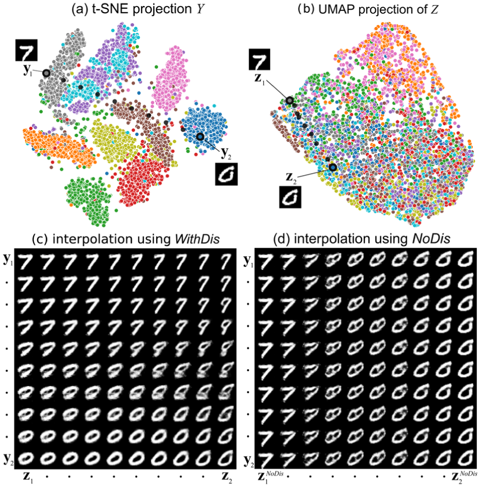
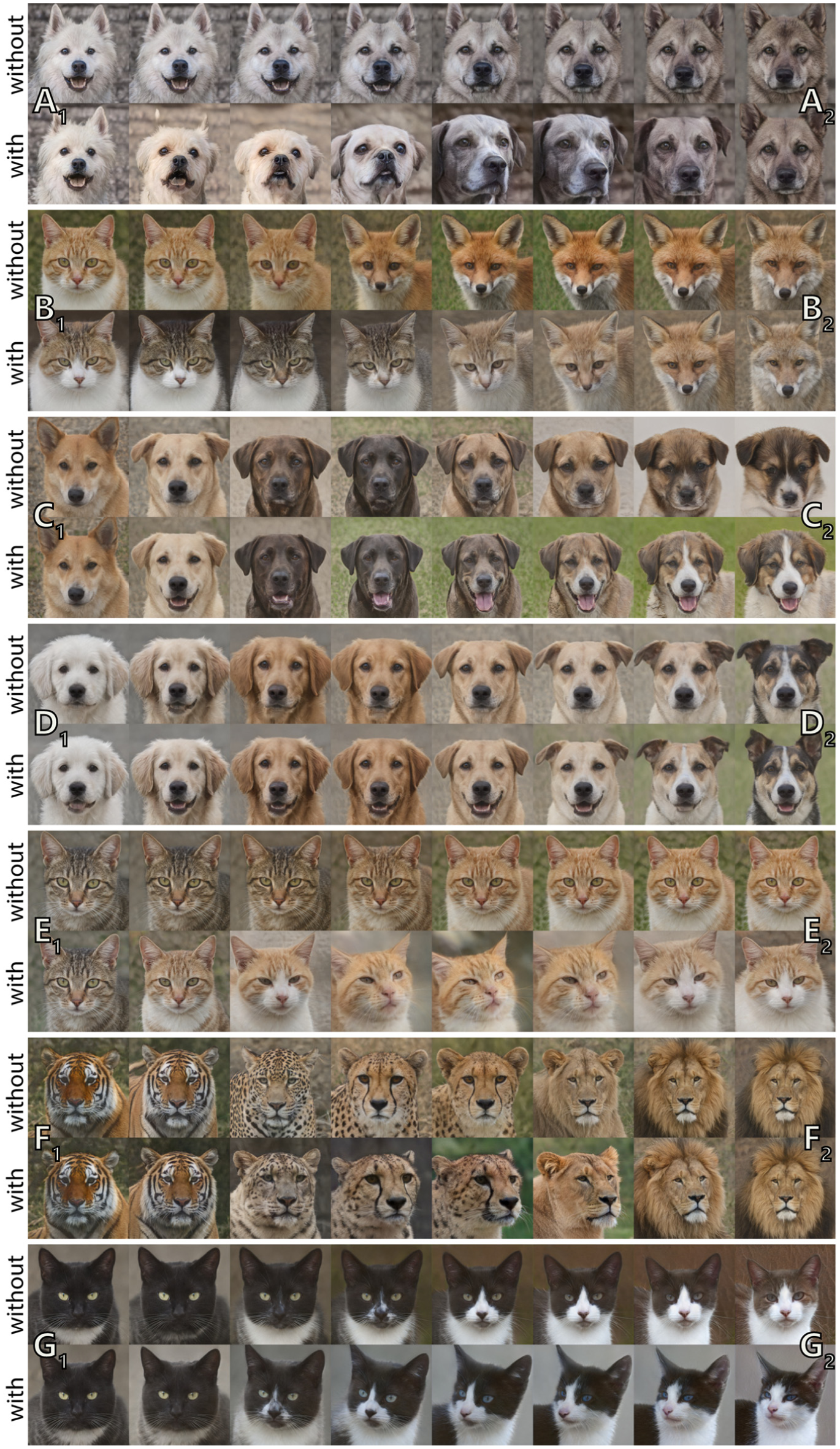
Qualitative evaluation: We visually evaluate disentanglement by selecting two samples $x_{1}$ and $x_{2}$ of MNIST dataset and their t-SNE projections $y_{1}$ and $y_{2}$ . These are two images of digits 0 and 7 – see Figure 4(a). Let $z_{1} = Enc (x_{1})$ and $z_{2} = Enc (x_{2})$ be the codes of these two images. These are shown in a UMAP projection of the $z$ values for the dataset in Figure 4(b). We linearly interpolate between $y_{1}$ and $y_{2}$ , and $z_{1}$ and $z_{2}$ , respectively, with 10 steps. This yields $10^{2}$ interpolated values $(y, z)$ which we inversely project to the data space using both WithDis (Figure 4(c)) and NoDis (Figure 4(d)). We see from the t-SNE projection that the label information is well-preserved in the projection space (Figure 4(a)) – that is, digits of the same type, for example, zeroes or sevens, are well grouped. In contrast, the UMAP projection of $z$ strongly mixes labels (Figure 4(b)). This is desired, as $z$ should capture a digit’s writing style and not its class. We next see that, as we change $z$ using WithDis, the digit’s style changes – see columns in Figure 4(c); while, as we change $y$ , the digit itself changes – see rows in Figure 4(c). Hence, WithDis disentangles $y$ and $z$ well. In contrast, for NoDis, the inverse projection changes only when $z$ changes – see columns in Figure 4(d); when $y$ changes, the digit stays the same – see rows in Figure 4(d). Hence, NoDis keeps the latent codes $z$ and $y$ entangled.

Figure 4.

Showing disentanglement on the MNIST dataset. (a) 2D t-SNE projection $Y$ . (b) UMAP projection of $Z$ using $WithDis$ . (c) Inverse projections of the linear interpolation between two data points in the $Z$ and $Y$ spaces, using $WithDis$ (c) and $NoDis$ (d).

Comparison to other inverse projection methods

We now compare our inverse projection LCIP to iLAMP,⁹ RBF,¹⁸ and NNinv.²⁴ We show that LCIP yields similar if not higher quality even without using its control mechanism (which we discuss separately in section ‘Controllability: Going beyond a fixed surface’).

Inverse projection error: We first measure the Mean Squared Error (MSE) of the inverse projection on the test set $D_{v}$

MSE = \frac{1}{| D_{v} |} \sum_{(y, x) \in D_{v}} ∥ x - P^{- 1} (y, z) ∥^{2},

(9)

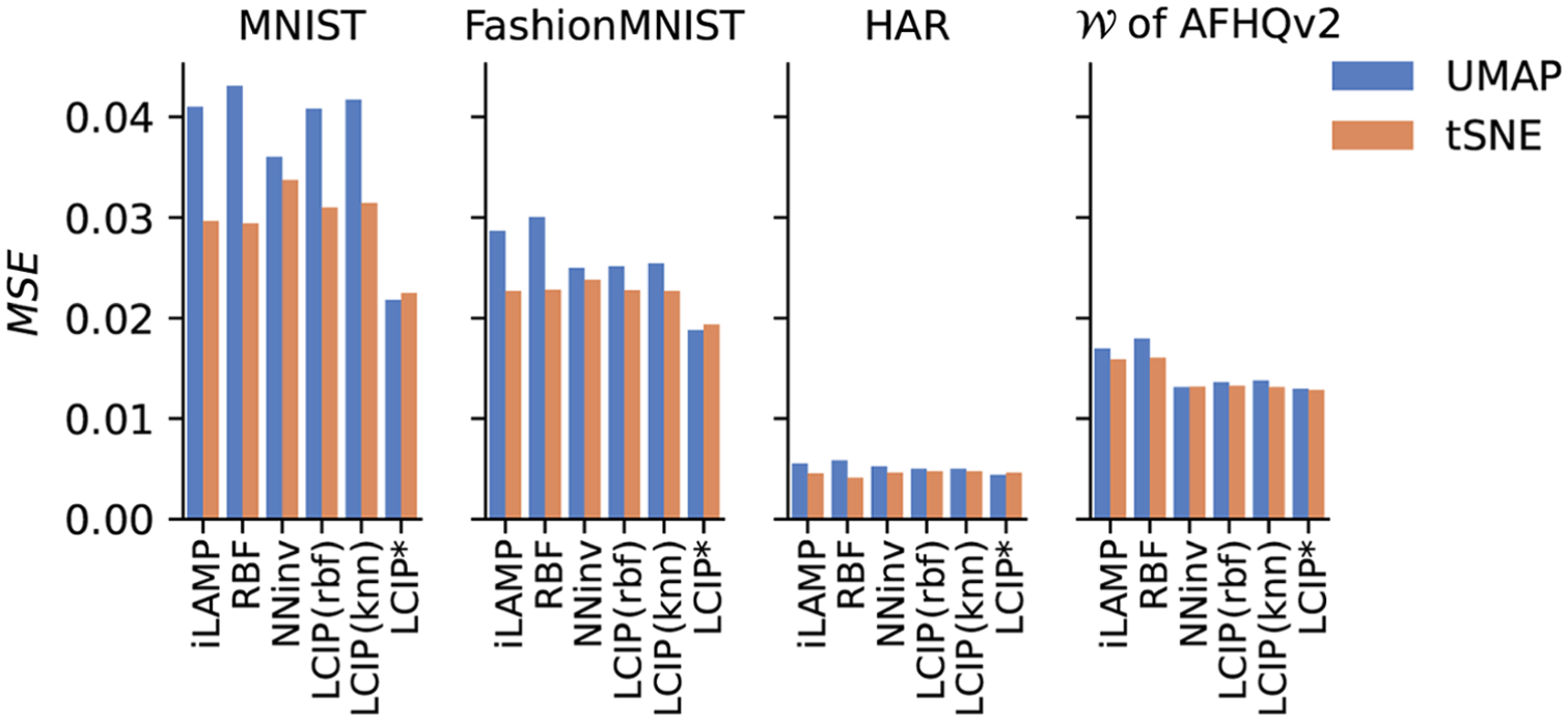
where $z$ is ignored for iLAMP, RBF, and NNinv. For LCIP, we compute $z$ at $y \in R^{2} ∖ Y$ by smoothed RBF and weighted k-NN interpolation of $z_{i}$ (section ‘Computing $z$ for the entire projection space’). We call these two variants LCIP (rbf) and LCIP (knn), respectively. We also compute $z_{i} = Enc (x_{i}), x_{i} \in X_{v}$ and denote it by LCIP*. While this is not the intended way to get $z$ (as we cannot do this for any 2D point, see section ‘Computing $z$ for the entire projection space’), this measures the quality of our method if we could compute $z$ exactly. Figure 5 shows that iLAMP, RBF, NNinv, and LCIP have similar MSE on $D_{v}$ . Yet, LCIP* has a lower MSE on MNIST and Fashion-MNIST. Hence, our method can produce inverse projections with lower error when $z$ is properly provided. The quality gap between LCIP* and LCIP (rbf) or LCIP (knn) can be filled by interaction (see next section ‘User control of the inverse projection’).

Figure 5.

MSE of the studied inverse projections.

Visual quality in gap areas: MSE testing can only be done for points in $D_{v}$ , where we have ground truth samples for $P^{- 1}$ . Yet, one wants to use inverse projections precisely in the gaps between 2D projected points (section ‘Projections and inverse projections’). One way to assess quality there is to study how inversely projected samples from gap areas look like. Ideally, we want to get plausible samples which follow the overall nature of the data in a given dataset.

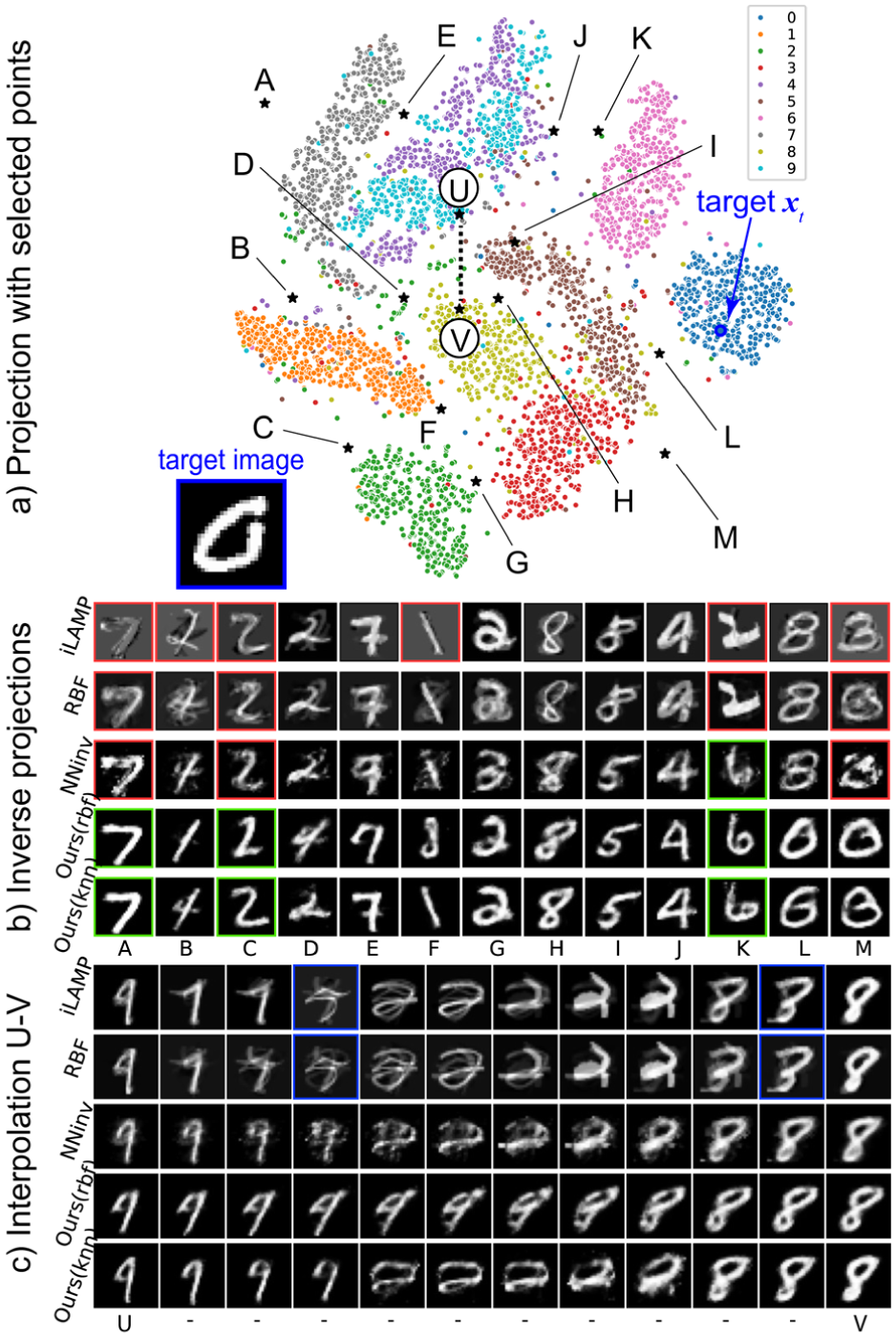
Figure 6 shows the four studied $P^{- 1}$ methods on MNIST. Images (b) show that LCIP produces more plausible digits than the other methods even at locations far away from data samples (e.g. A, C, M). We also see that iLAMP and RBF are more sensitive to outliers. For example, consider the green point (near K, class 2) located in between the pink (class 4) and purple (class 6) clusters, while the main green cluster is down at the bottom of the projection. The inverse projection of ‘K’ (close to the green point) is a ‘2’ in iLAMP and RBF, while it is a ‘6’ in NNinv and LCIP, so iLAMP and RBF feel the effect of this single outlier strongly whereas NNinv and LCIP do not. Separately, iLAMP creates gray backgrounds (e.g. A, B, C, F, M) which are not only far away from the actual data distribution but also not what one would expect for MNIST. Images (c) show the inverse projections from points along a line between images U (digit 9) and V (digit 8) in the projection. iLAMP, RBF, and NNinv generate spurious shapes that do not resemble any digit during this interpolation process – this is very likely due to the few outlier points from different classes present along this line. In contrast, LCIP morphs the 9 to an 8 following, we argue, a more natural set of intermediate images. As such, if one desires an inverse projection which is less sensitive to outlier points, LCIP is preferable.

Figure 6.

Visual comparison of inverse projection, MNIST dataset. (a) 13 points A-M are selected in the projection space at various distances from projected samples. (b) The inverse projections at these locations using the tested inverse projection techniques. (c) Results obtained by inversely projecting points along a line between the locations U and V in the projection.

A further way to test inverse projection quality in gap areas would check whether $P (P^{- 1} (p)) = p$ for points $p$ in such gaps – that is, whether images created by LCIP would be placed by $P$ at the 2D locations from where they were inferred. However, this requires a parametric projection function $P$ . We do not want to impose such constraints on our pipeline but rather allow users to pick any technique $P$ – in particular, t-SNE; as such, we do not perform the above-mentioned test.

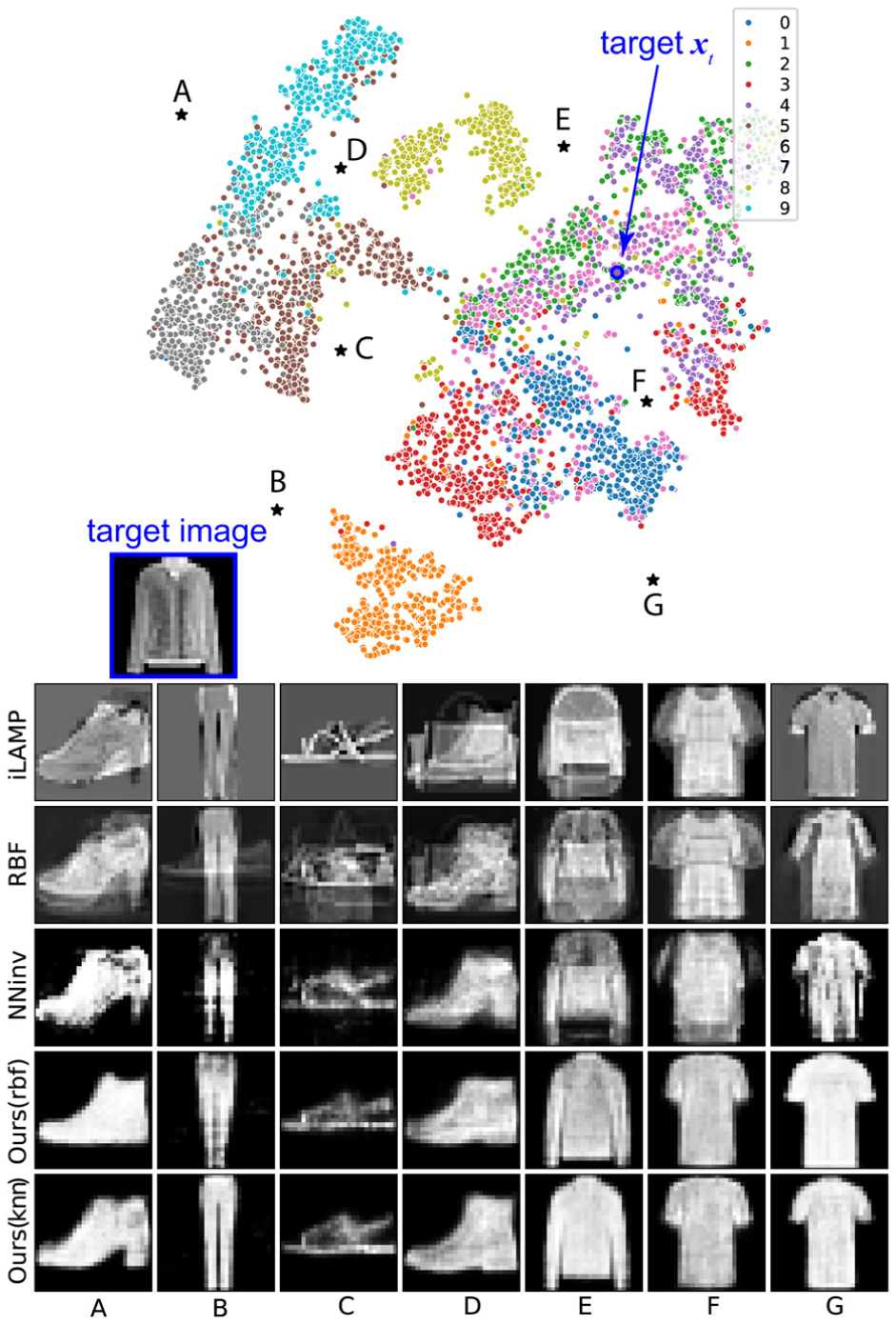
On Fashion-MNIST, iLAMP and RBF mix several images in the reconstruction (Figure 7). For example, at point A, iLAMP and RBF mix high heels and boots; at point B, RBF mixes shoes and pants; at point F, iLAMP and RBF mix a wider and a narrower T-shirt. NNinv doesn’t have this problem, but it produces jagged (e.g. at points A, B, C, G) or ambiguous shapes (e.g. at points E, F). LCIP keeps the reconstructed shape clear and recognizable in all cases.

Figure 7.

Visual comparison of the inverse projection, Fashion-MNIST dataset.

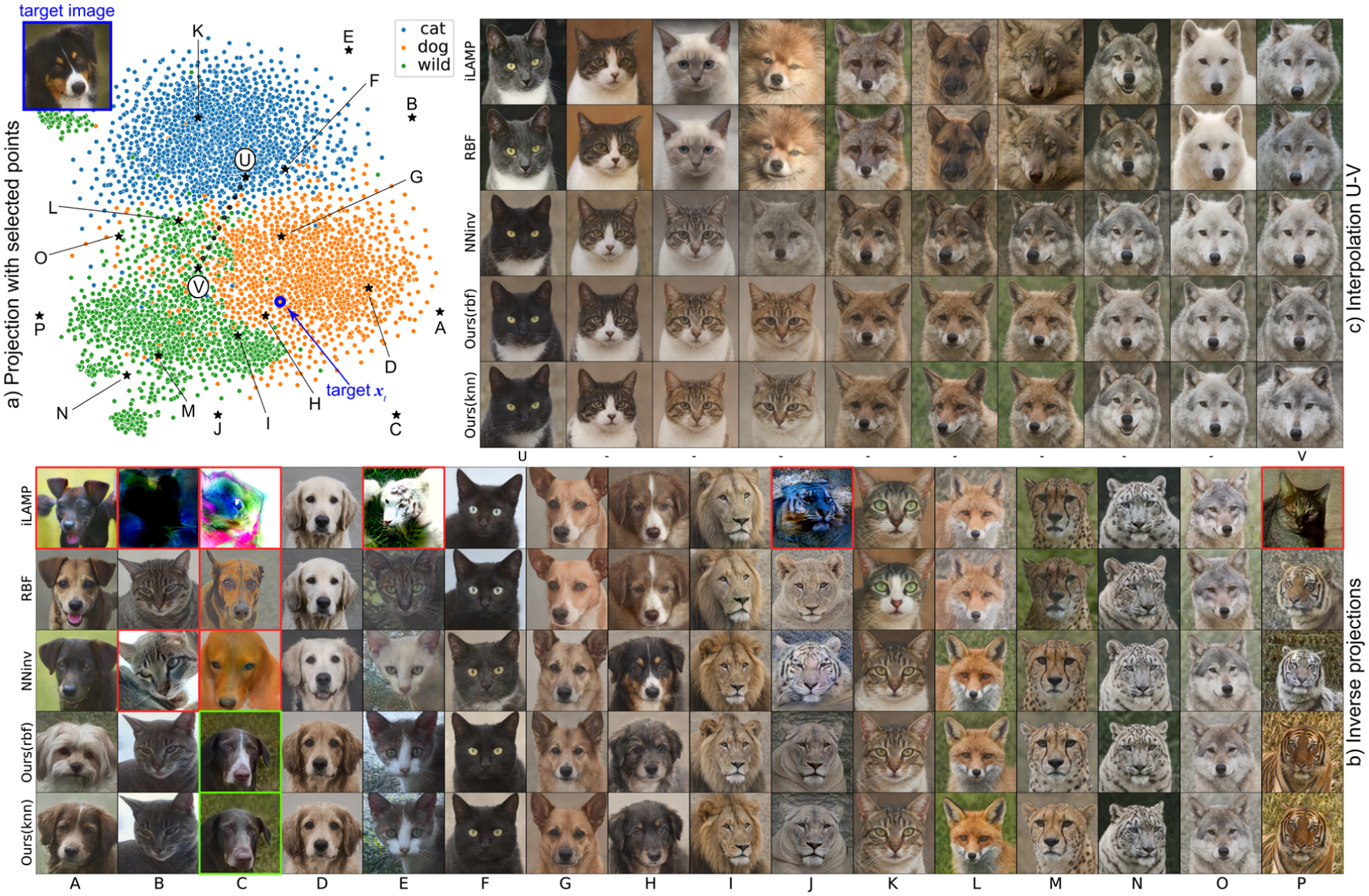
On AFHQv2, all tested $P^{- 1}$ methods work well when the inversely-projected 2D points are close to training samples. Once a 2D point is further away, iLAMP becomes problematic (see A, B, C, E, J, P). In extreme cases, all methods but ours have issues. For example, at point C (Figure 8), iLAMP produces a mass of colors with indiscernible shapes; RBF produces color distortions and a dog with only one ear; NNinv produces a dog but in a strange appearance, also with color distortions. In contrast, LCIP produces realistic images in all cases.

Figure 8.

Visual comparison of inverse projections, AFHQv2 dataset. (a) Dataset projection with 16 selected locations both close and far away from data samples (A–P). (b) Inverse projections at A–P created by all tested methods. (c) Inverse projections of points on a line between locations U and V in the projection.

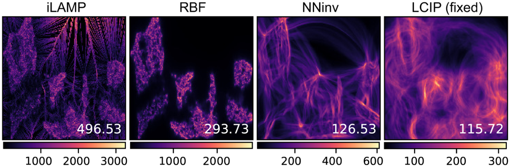
Smoothness comparison: We next evaluate smoothness using gradient maps.¹⁰ These are images which depict the gradient norm $∥ \nabla P^{- 1} (p) ∥$ at every pixel $p$ of the projection space. Figure 9 shows these maps for the tested inverse projections on MNIST with the UMAP projection; additional datasets and projections, shown in the supplementary material, follow the same pattern. Bright colors (high gradients) show points where the inverse projection ‘jumps’ in data space when its input moves between neighbor pixels. Such jumps are undesirable (see section ‘Projections and inverse projections’). We see that LCIP achieves the smallest gradient norms (see color legends) for all datasets and direct projections.

Figure 9.

Gradient maps for the tested inverse projections for UMAP on MNIST.

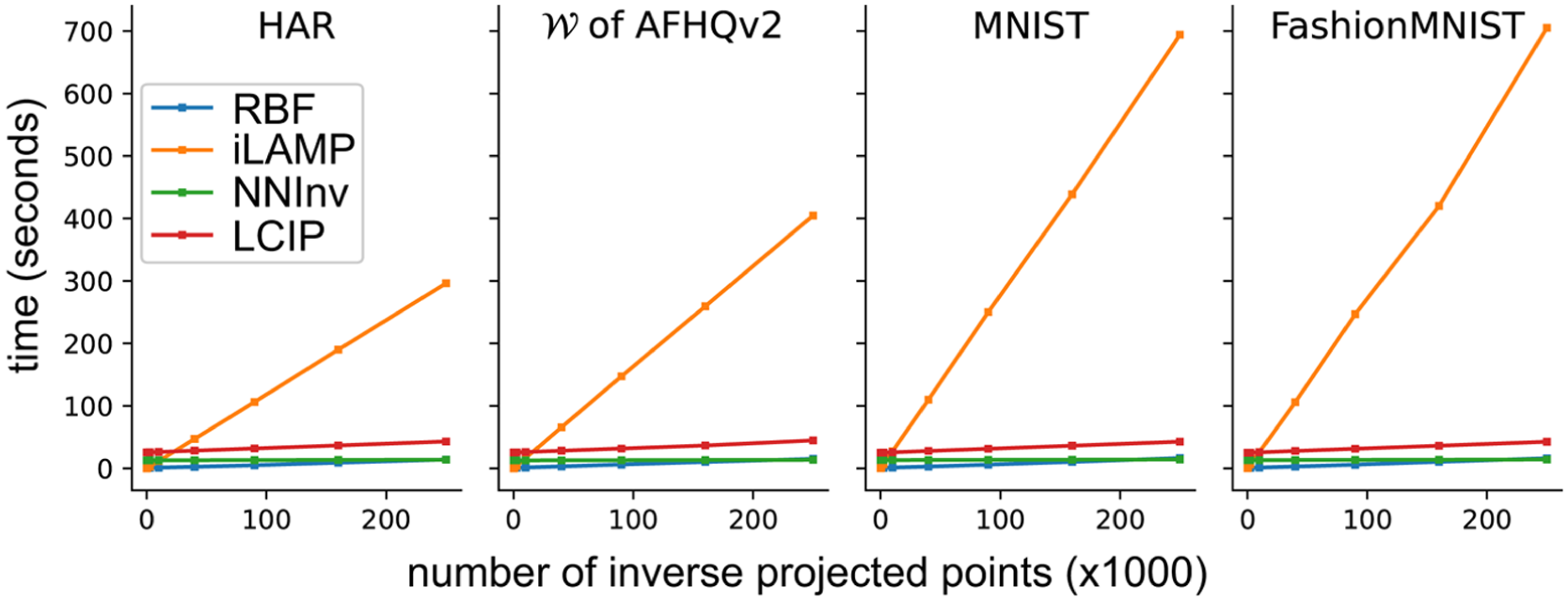
Computational speed: Figure 10 shows timings for the four studied inverse projection methods on a PC with an Intel Core i5-12400 CPU and NVIDIA GeForce RTX 3090 GPU. The y-axis shows the (constant) training time plus inference time (linear in the projected points count). All methods show similar speed except iLAMP which is visibly slower. Although LCIP requires slightly more training time due to its adversarial training, its slope is nearly identical to NNinv and RBF, showing the same high scalability. Separately, our evaluations show that the results of LCIP (rbf) and LCIP (knn) are very similar. Since LCIP (rbf) is theoretically smoother, we will use it in our following experiments.

Figure 10.

Inverse projection speed. Training time is the y-intercept on the charts. Line slopes show how inference time depends on the number of inversely projected samples.

Controllability: Going beyond a fixed surface

We have shown so far that LCIP can construct a ‘fixed’ inverse projection from a given dataset $X$ and its projection $P (X)$ with results which are comparable – and often better – than other existing inverse projection techniques in terms of generating plausible results in gap areas, inverse projection MSE, inverse projection smoothness, and speed. Yet, the key feature of our method is its ability to dynamically control the inverse projection, which we describe next.

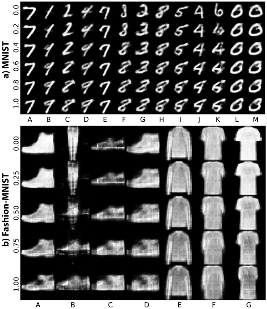
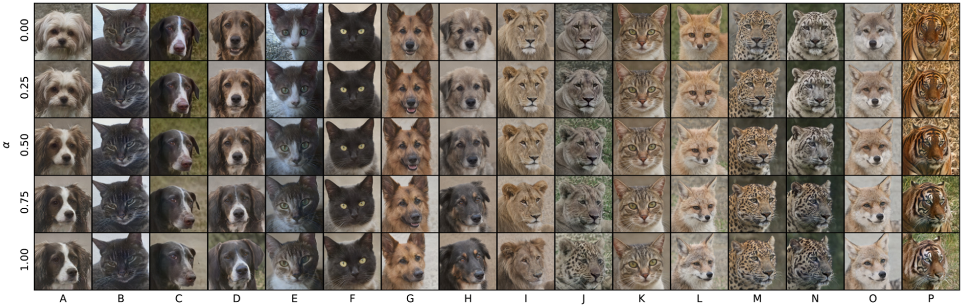
Control effects: Figures 11 and 12 show how the inverse projection changes when $z$ values are adjusted towards selected targets in MNIST, Fashion-MNIST and AFHQv2. Targets are marked by $x_{t}$ (blue) in Figures 6 –8 with their images shown as insets. In Figures 11 and 12, topmost rows show the selected source images $(α = 0)$ ; rows below show how the inverse projection ‘sweeps’ the data space between source and target as the user increases $α$ . For example, when selecting an italic-like ‘0’ digit in MNIST as target and increase $α$ , the inverse projections gradually become more italic, no matter which source image is selected (Figure 11). We see similar changes in Fashion-MNIST, see the subtle changes in shoe and shirt styles (Figure 11 bottom). For AFHQv2, the target is a dog tilting its head (inset image in Figure 8). As we increase $α$ , all selected source animals in the inverse projection rotate their heads with similar angles (Figure 12).

Figure 11.

Controlling the inverse projection for MNIST (a) and Fashion-MNIST (b). Targets are the blue-outlined inset images in Figure 6 for (a) and Figure 7 for (b). Rows in the two images show the effect of increasing user control $α$ .

Figure 12.

Controlling the inverse projection for AFHQv2. The target is the blue-outlined image in Figure 8.

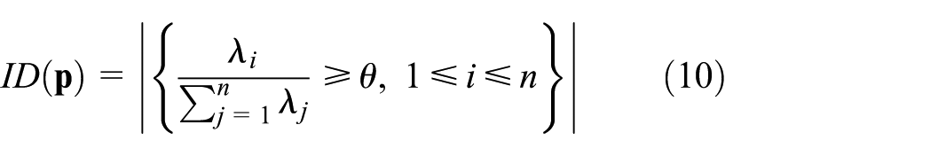
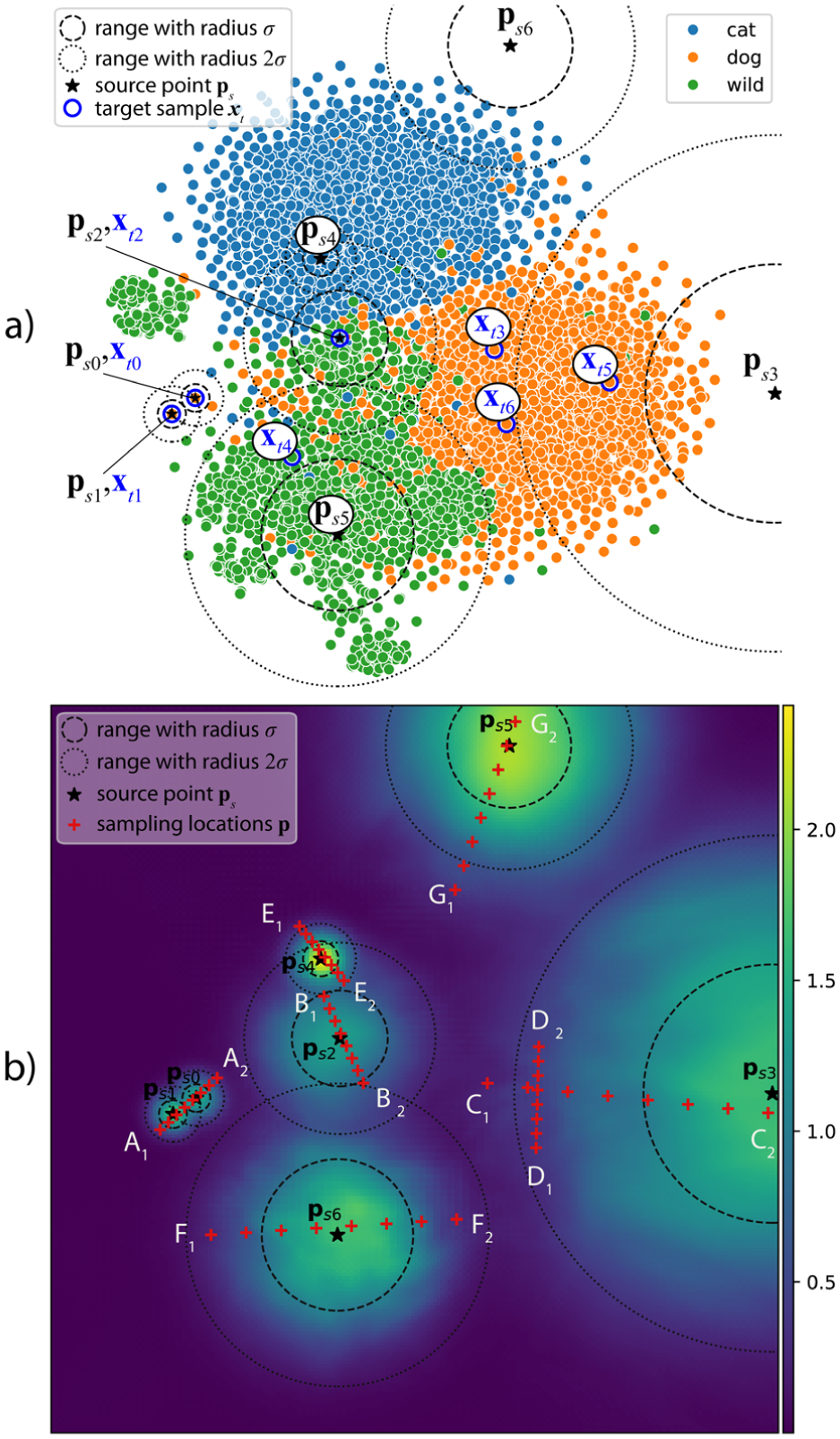
Increased reach: While LCIP generates inverse projections that go beyond a fixed surface, a key question is how much beyond such a surface it can reach. To quantify this, we evaluate the Intrinsic Dimensionality (ID) of the inverse projection (run without interaction) using the Minimal Variance method.⁴⁸ In detail, we sample a set $A$ of $100 \times 100$ pixels in the 2D projection space and map these through LCIP (without interaction) to get $Q = {q_{ℓ} = P^{- 1} (p_{ℓ}) | p_{ℓ} \in A} \subset R^{n}$ . For each query pixel $p$ , we consider its inverse $q = P^{- 1} (p)$ and define the neighborhood $S (p) = {q_{ℓ} \in Q ∣ ∥ q - q_{ℓ} ∥_{2} \leq r}$ , where $r = 0.1 \cdot \max_{q_{i}, q_{j} \in Q} ∥ q_{i} - q_{j} ∥_{2}$ sets a fixed-radius neighborhood in data space. We assess how close $S (p)$ is to an embedded surface by computing the eigenvalues $λ_{i}$ , $1 \leq i \leq n$ , of the covariance matrix of $S (p)$ , sorted in descending order, and then evaluate

ID (p) = | {\frac{λ_{i}}{\sum_{j = 1}^{n} λ_{j}} \geq θ, 1 \leq i \leq n} |

(10)

with $θ = 0.05$ . $ID (p)$ counts how many principal directions each explain at least a fraction $θ$ of the total variance of $S$ . If $ID (p)$ is close to $2$ , it means that the inverse projection locally creates a surface around the backprojection of pixel $p$ and its neighbors. We call this ID value the baseline.

Next, we adjust LCIP by globally adding $Δ z$ values via equation (8), for 50 uniformly sampled values of $α \in [0, 0.2]$ (yielding $| Q | = 5 \times 10^{5}$ ), and use equation (10) to measure the ID of all these $5 \times 10^{5}$ inversely-projected pixels taken together.

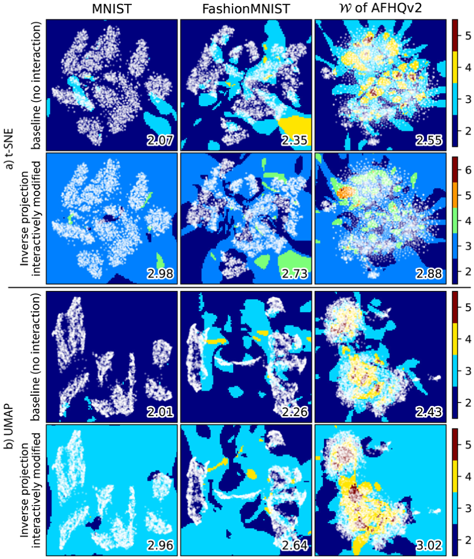
Figure 13 shows that the baseline has $ID \approx 2$ at roughly all pixels of the sampled projection space (with small higher-ID areas close to the sample points). Figures in the bottom-right corners of the images show the average $ID$ over all projection space pixels. We see that, when using LCIP without user control, LCIP creates roughly a surface embedded in $R^{n}$ , much like other inverse projection techniques.¹⁴ When using control, we get an ID roughly equal to 3, that is, $Δ z$ ‘shifts’ our inverse-projection surface to span a 3D space in $R^{n}$ . Some ID values of 2 are likely due to the $z$ value of those areas being insensitive to the selected target, that is, $z_{t}$ and $z_{p_{s}}$ are close in the first place. Note that we only use a single target point here. If we used $T > 1$ target samples $x_{t}$ which span a $T$ -dimensional space in $R^{n}$ , we would obtain an inverse projection of $ID \approx T$ . Figure 15, (discussed later in this section) shows the same effect: changing $α$ pulls the inversely projected surface into areas far outside the original fixed surface, confirming the increased reach measured above.

Figure 13.

Intrinsic dimensionality of LCIP without and with interaction for different datasets and direct projections.

Flexible control: We further study the impact of using more control targets $x_{t}$ . For this, we consider a training set $X_{T}$ with 5000 points. For each $x_{i} \in X_{T}$ , we compute its latent code $z_{i} = Enc (x_{i})$ , consider it as a target for our control mechanism, and consider each pixel $p$ of the projection space as source point. For each such $p$ , we measure the variance

V (p) = \frac{\sum_{j = 1}^{n} V ar ({P^{- 1} (p, z_{i})}^{j})}{\sum_{j = 1}^{n} V ar (X_{T}^{j})} .

(11)

over the set ${Dec (p, z_{i})}$ , across all data dimensions $1 \leq j \leq n$ . Higher values of $V (p)$ indicate that the inverse projection of $p$ is more sensitive to control, and vice versa. The denominator in equation (11) accounts for the spread of the training set $X_{T}$ in data space. If this spread is low, we should not expect that our inverse projection reaches far in the data space, and vice versa.

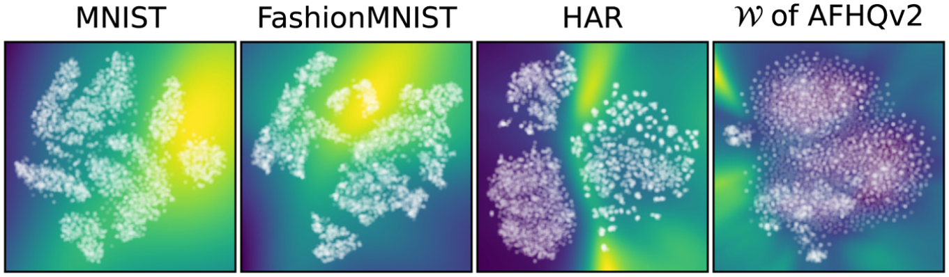
Figure 14 shows the results. On $W$ of AFHQv2 and HAR, variance is lower near data samples and higher in gap areas, telling that inverse projections are more ‘nailed’ when there is ground-truth data around, and more flexible when there is no ground truth nearby. On MNIST and Fashion-MNIST, the pattern seems not to be related to the distance to data samples. We believe that this is an effect of t-SNE’s known tendency to compress (or stretch) point neighborhoods from data space to projection space.⁴⁹ That is, areas showing a low normalized variance in Figure 14 may actually map points which are close in data space, where our inverse projection does not have the freedom to move much; conversely, areas of high variance may map points far away in data space, where our inverse projection has more freedom to move. These maps provide users with insights on where interaction is likely to be most effective: Interacting with source points in high-variance areas will produce inverse projections which ‘sweep’ the data space more freely, which is the core goal of interaction; interacting with source points in low-variance areas is likely not going to discover new areas in data space.

Figure 14.

Normalized variance of inverse projections produced by 5000 different $z$ values, t-SNE direct projection. See equation (11) and related text.

Exploring decision maps: As mentioned in section ‘Background and related work’, inverse projections are a key element to compute decision maps which are used to depict the behavior of trained classification models of the type $f : R^{n} \to C$ .^7,8,11 A decision map colors all pixels $p$ of the projection space by $f (P^{- 1} (p))$ . As explained, existing inverse projections only depict the model’s behavior on a single, fixed surface embedded in $R^{n}$ . How the model behaves outside of this surface is left unexplored.

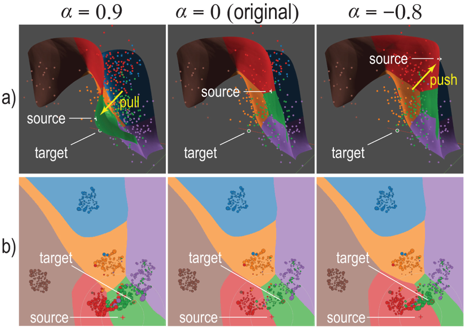
LCIP allows users to interactively change this surface to explore specific data-space regions close to samples of interest and in directions of interest. Figure 15 shows this using a synthetic 3-dimensional dataset with 6 classes and a lightweight fully connected classifier (mirroring the setup presented in Wang and Telea¹⁴). Since $n = 3$ , we can directly visualize the inversely projected surface created by LCIP. The middle column of Figure 15 shows the fixed surface and corresponding decision map for $α = 0$ , that is, similar to other inverse projection methods. We would now like to explore the behavior of the classifier outside this surface – more specifically, close to the sample marked source and in the direction towards the sample marked target. We first use $α = 0.9$ to pull the surface from source towards target. The left column of Figure 15 shows how the surface locally deforms accordingly; this effectively demonstrates the effect outlined earlier in Figure 3. At the same time, the decision map changes to show us how the model behaves in previously unseen areas in data space that the deformed surface goes through now. Next, we set $α = - 0.8$ to push the surface from source away from the target, as shown in the right column of Figure 15. This explores the model on the other side of the original fixed surface. Interactively changing $α$ allows us to see the model’s behavior on a dense set of surfaces which sweep the data space around the source and in the positive/negative direction of the target. Choosing different sources and targets enriches our understanding of the visualized classifier in specific areas of interest.

Figure 15.

(a) Inversely projected surface and (b) corresponding decision maps produced by LCIP for a synthetic 3D six-class blob dataset and classified by a 3-layer fully connected deep-learning network (hidden layers of size 512/256/128). Users can vary $α$ to ‘sweep’ the 3D space with the inversely projected surface and corresponding decision maps.

User control of the inverse projection

We now show how the control of LCIP works in practice using the tool shown in Figure 1(a). Based on how far the selected source $p_{s}$ is from the selected target $P (x_{t})$ in projection space, we have in practice two types of control: target is (1) close to, respectively (2) far away from, the source. In (1), we expect $P^{- 1}$ to gradually but fully change towards the target; In (2), we only expect a partial change, for example, style-wise. We show next that LCIP yields indeed these two different effects.

Local control: Target is close to source

We next show how our control helps with two challenges that frequently occur in inverse projection usage when the target $x_{t}$ projects close to the source $p_{s}$ . Consider first the limit case where $P (x_{t}) = p_{s}$ . The difference between the target $x_{t}$ and the controlled inverse projection $Dec (p_{s}, z_{p_{s}})$ is fully controlled by $z_{p_{s}}$ . When $z_{p_{s}} = Enc (x_{t})$ , the inverse projection of $p_{s}$ becomes $Dec (P (x_{t}), Enc (x_{t})) \approx x_{t}$ , that is, the inverse projection fully changes towards the target $x_{t}$ .

Now consider the case where $x_{t}$ projects close to, but not exactly at, the source $p_{s}$ . In the following, note that the choice of the target $x_{t}$ is application dependent, that is, depends on towards which data sample of special interest one wants to locally ‘pull’ the projection.

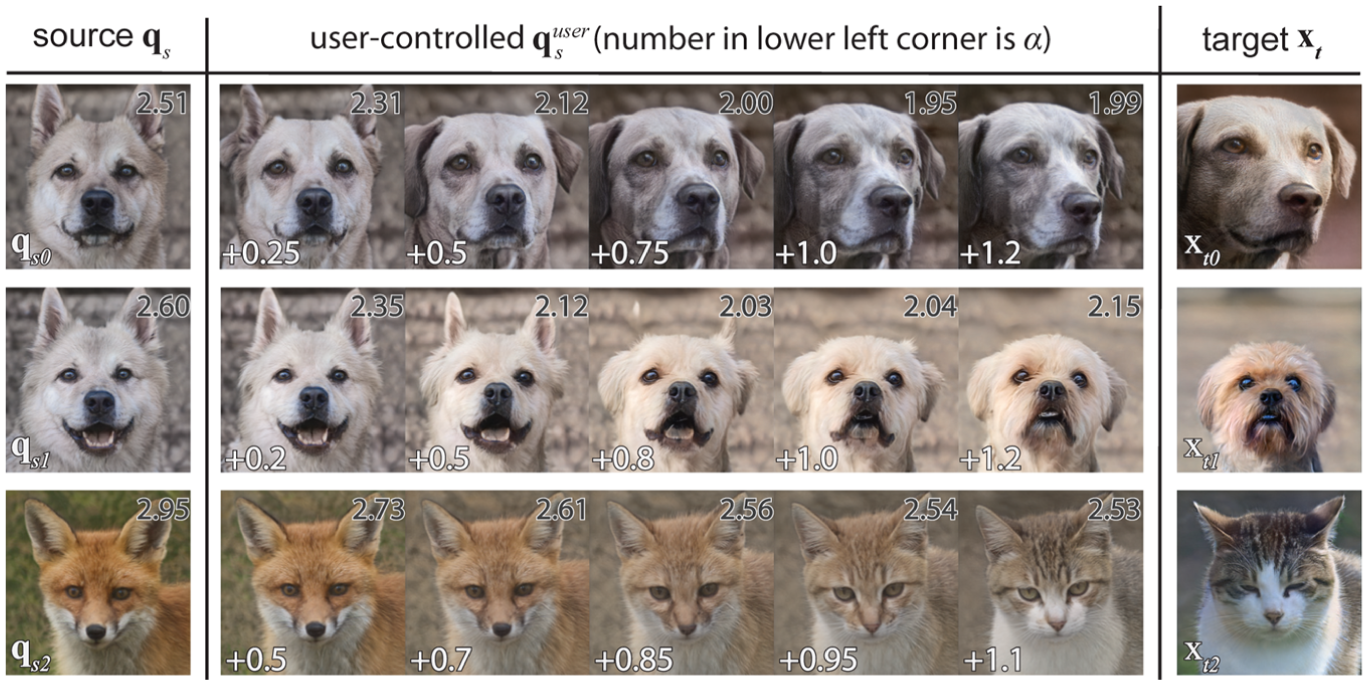
Inverse projection correction: While good inverse projections should have a low MSE (equation (9)), they do not yield $P^{- 1} (P (x)) = x$ at all projected samples $P (x)$ . For instance, in Figure 16(a), $p_{s 0} = P (x_{t 0})$ and $p_{s 1} = P (x_{t 1})$ are two points at the margin of clusters. As such, their inverse projections $q_{s 0} = P^{- 1} (p_{s 0})$ and $q_{s 1} = P^{- 1} (p_{s 1})$ should not be strongly influenced by other points; ideally, $q_{s 0}$ and $q_{s 1}$ should equal the samples $x_{t 0}$ and $x_{t 1}$ that project there. Yet, this is not the case: The inverse projection images $q_{s 0}$ and $q_{s 1}$ are not similar to the sample images $x_{t 0}$ , $x_{t 1}$ (Figure 17). We can control our inverse projection to make it closer to the data. As we add $Δ z$ to $z_{p_{s}}$ with higher $α$ values, the inverse projection $q^{user}$ gradually changes towards the target $x_{t}$ – see Figure 17 top two rows. The distances $∥ q^{user} - x_{t} ∥$ are also reduced, reaching minima for $α = 1$ (Figure 17).

Figure 16.

Close and far-away control of the inverse projection, AFHQv2 dataset. (a) 2D locations where we performed interaction. See also Figures 17 and 18. (b) Assessing smoothness of controlled inverse projection at various sampling locations (+). Color encodes the distance $∥ q - q^{user} ∥$ at each pixel. Figure 19 shows the inverse projections at these sampling locations.

Figure 17.

Local control – adjusting the inverse projection when $P (x_{t}) \approx p_{s}$ . Locations of $q_{s}$ and $P (x_{t})$ are shown in Figure 16(a). Numbers in upper right corners show $∥ x_{t} - q_{s}^{user} ∥$ . Numbers in lower left corners show the control parameter $α$ .

Overlap separation: Overlapping points in a projection are common. More precisely, projection techniques can place samples which are (very) far apart in data space very close in the projection space – in the limit, such points can even overlap given the finite size used to draw points in a visualization. This can be quantified by various projection quality metrics for example, trustworthiness.^50,51 For example, in Figure 16(a), the area around point $p_{s 2}$ – which corresponds to a cat (denoted $x_{t 2}$ ) – shows overlapping samples of cats (blue) and wild animals (green). This overlap is due to the projection – the samples are actually separable in data space. Existing inverse projection methods will map $p_{s 2}$ to a cat, a wild animal, or a mix of them in a fixed and uncontrollable way. Our method allows controlling the inverse projection of $p_{s 2}$ to be more like a cat or a wild animal: We see that $q_{s 2}$ is initially a fox (Figure 17, bottom row, left). Setting the cat image $x_{t 2}$ as the target and $p_{s 2}$ as source, we see how the inverse projection gradually transforms from a fox into a cat as we increase $α$ (Figure 17, bottom row, columns $q_{s}^{user}$ ).

Far-away control: Target is far from source

In this scenario, the controlled $P^{- 1} (p_{s}, z_{p_{s}})$ will not go completely toward $x_{t}$ , since $P (x_{t}) \approx p_{s}$ . Rather, only what is controlled by $z$ will change. It is important to note that it is hard to tell, in general, what $z$ exactly controls as this depends on what is lost in the projection $y$ , which in turns depends on the actual projection technique $P$ used and on the dimensionality of the input data. Our specific claim is thus: Given that there is such a loss, we (1) capture this loss and (2) allow users to ‘put it back’ in the computation of the inverse projection – unlike existing inverse projection techniques which behave as if this loss would not exist.

We illustrate the above with a few examples. In our studies, we found that, for the MNIST–t-SNE combination, the digit is controlled by $y$ , while $z$ controls the digit’s style; for the AFHQv2–t-SNE combination, the type of animal faces is controlled by $y$ , while the animal poses are controlled by $z$ . Controlling $z$ shapes the inverse-projected surface as desired, enabling user-controlled data generation, as illustrated next.

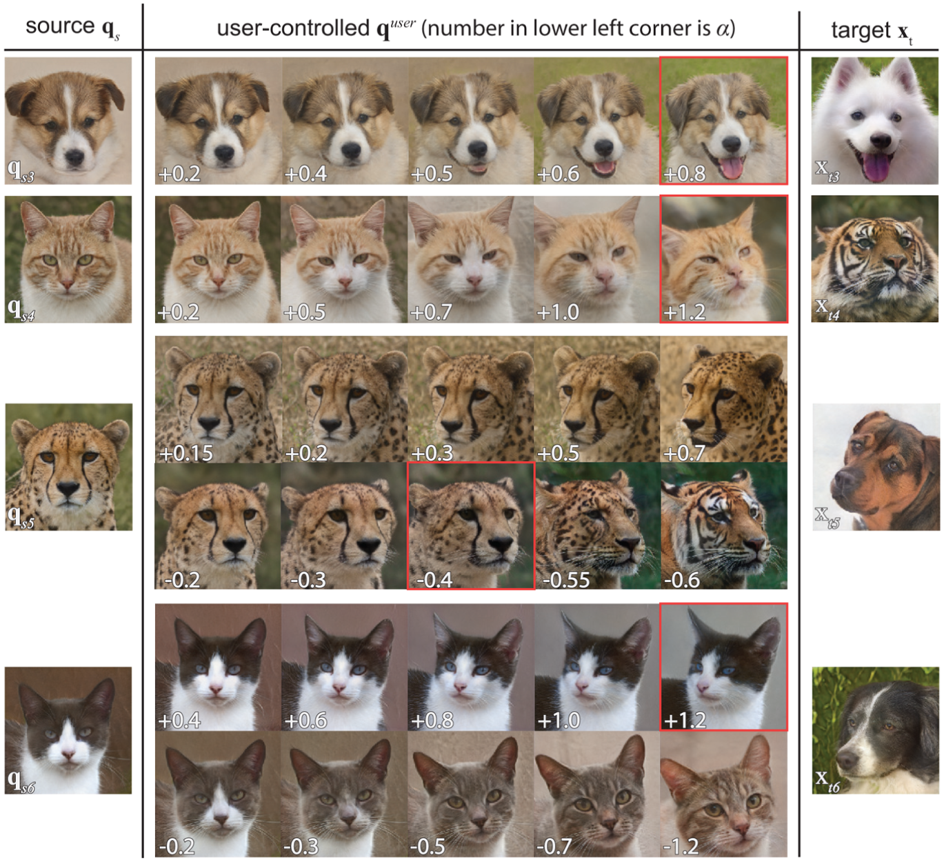
Consider a source $p_{s}$ far from any target, that is, in a gap area in the projection. All existing inverse projection techniques produce surface-like structures in such areas (section ‘Projections and inverse projections’). Our control breaks this limitation: Take point $p_{s 3}$ which is in a gap area (Figure 16(a)). Its inverse projection is a sad-looking puppy ( $q_{s 3}$ , Figure 18 top-left). We now pick as target a happy dog ( $x_{t 3}$ , Figures 16(a) and 18 top-right). As we increase $α$ , the sad puppy gradually smiles and finally laughs with open mouth (Figure 18, $q^{user}$ , top row). Note that the puppy’s appearance, for example, hair color and ear shapes, do not change to the target – only its ‘style’ changed. This control also works with source and target from different classes. The inverse projection $q_{s 4}$ of $p_{s 4}$ is a cat looking ahead (Figure 18, left column, second-top image). We choose as target a tiger looking up ( $x_{t 4}$ in Figure 18, right column, $2 nd$ top image). By increasing $α$ , the cat gradually looks up without becoming a tiger (Figure 18, $q^{user}$ , $2^{nd}$ row).

Figure 18.

Far-away control – adjusting the inverse projection when $P (x_{t}) \approx p_{s}$ . Locations of $q_{s}$ and $P (x_{t})$ are shown in Figure 16(a).

Lowering $α$ has the opposite effect. Take a front-facing cheetah as source $p_{s 5}$ (Figure 18, left column, 3rd image from top); and a left-facing dog as target $x_{t 5}$ (Figure 18, right column, 3rd image from top). Increasing $α$ , the cheetah turns its head left (Figure 18, $q^{user}$ , row 3). Lowering $α$ , the cheetah’s head turns right (Figure 18, $q^{user}$ , row 4). At $α \approx - 0.55$ , the cheetah starts becoming a tiger, since cheetahs and tigers overlap in the projection. This $α$ decrease triggers overlap separation (section ‘Local control: Target is close to source’). Finally, we choose a source $p_{s 6}$ in a gap area whose $P^{- 1}$ is a black-and-white front-facing cat (Figure 18, left column, bottom image). We set as target a left-facing dog ( $x_{t 6}$ , Figure 18, right column, bottom image). Increasing $α$ , the cat’s head turns left (Figure 18, $q^{user}$ , row 5). Lowering $α$ , the cat’s head tilts right and fur changes color to brown (Figure 18, $q^{user}$ , row 6).

By adjusting $α$ , users can control subtle style features, such as the expression or direction a subject is facing, without altering a sample’s core identity. This ability extends across different classes and also far from any projected data sample. In other words, LCIP supports tasks such as user-controlled data generation where keeping the original data’s integrity, while introducing desired variations, is desired.

Smoothness of controlled inverse projections

Section Visual comparison of inverse projections, AFHQv2 dataset. (a) Dataset projection with 16 selected locations both close and far away from data samples (A–P). (b) Inverse projections at A–P created by all tested methods. (c) Inverse projections of points on a line between locations U and V in the projection. showed that LCIP without user control is smooth. User control should not affect this as $Dec$ ’s input smoothly varies with $p$ , $α$ and $σ$ (equation (8)) and $Dec$ itself is smooth (being the neural network outlined in section ‘Design of loss-controlled inverse projection’). Yet, let us test this in practice. We choose 7 source points $p_{s 0} \dots p_{s 6}$ and sample seven lines $A_{1} A_{2}$ … $G_{1} G_{2}$ in projection space with 8 samples each (Figure 16(b), samples: +; source points: ★). We next set different $α$ and $σ$ values for the source points and compute their inverse projections. Figure 19 shows the inverse projections without and with control. Images in each row – thus, over a set of per-line sampling points – smoothly change in both cases. To further confirm this, Figure 16b color-codes the difference between the inverse projection without and with control $∥ q - q^{user} ∥$ at each pixel. The result is a smooth signal, with large values close to the source points and small values further away, exactly as aimed by local control (equation (8)). Supplemental material Figure 2 supports this by showing gradient maps before and after user control. The smoothness of LCIP with user control is further confirmed by a user study (see section ‘User study: Evaluating LCIP in practice’, Task 3). Yet, Figure 19 shows that some image sequences change more rapidly than others – see for example, the sequence $C_{1} C_{2}$ , third row from top. This is explained by the fact that equal steps in projection space (Figure 16(b)) may map to small, or larger, steps in data space due to the nonlinearity of the used t-SNE projection.

Figure 19.

Smoothness with/without control: Inverse projections at 8 locations (columns) around 7 source points (rows). Images are ‘+’ marks in Figure 16(b).

User study: Evaluating LCIP in practice

We conducted a user study with 15 participants (P1–P15). We used four tasks to measure the Uniqueness (T1) and Fidelity (T2) of the generated data; and Smoothness (T3) and Controllability (T4) of LCIP. We used AFHQv2 (Figures 1 and 16), a complex but still interpretable dataset. T1–T2 follow Amorim et al.’s¹⁸ evaluation of inverse projections. T1–T3 used images printed on paper ( $5 \times 4.5$ cm) to ease task execution. For T4, participants used our tool; we collected user feedback on controllability and usability via post-task interviews. For full details, see supplementary material.

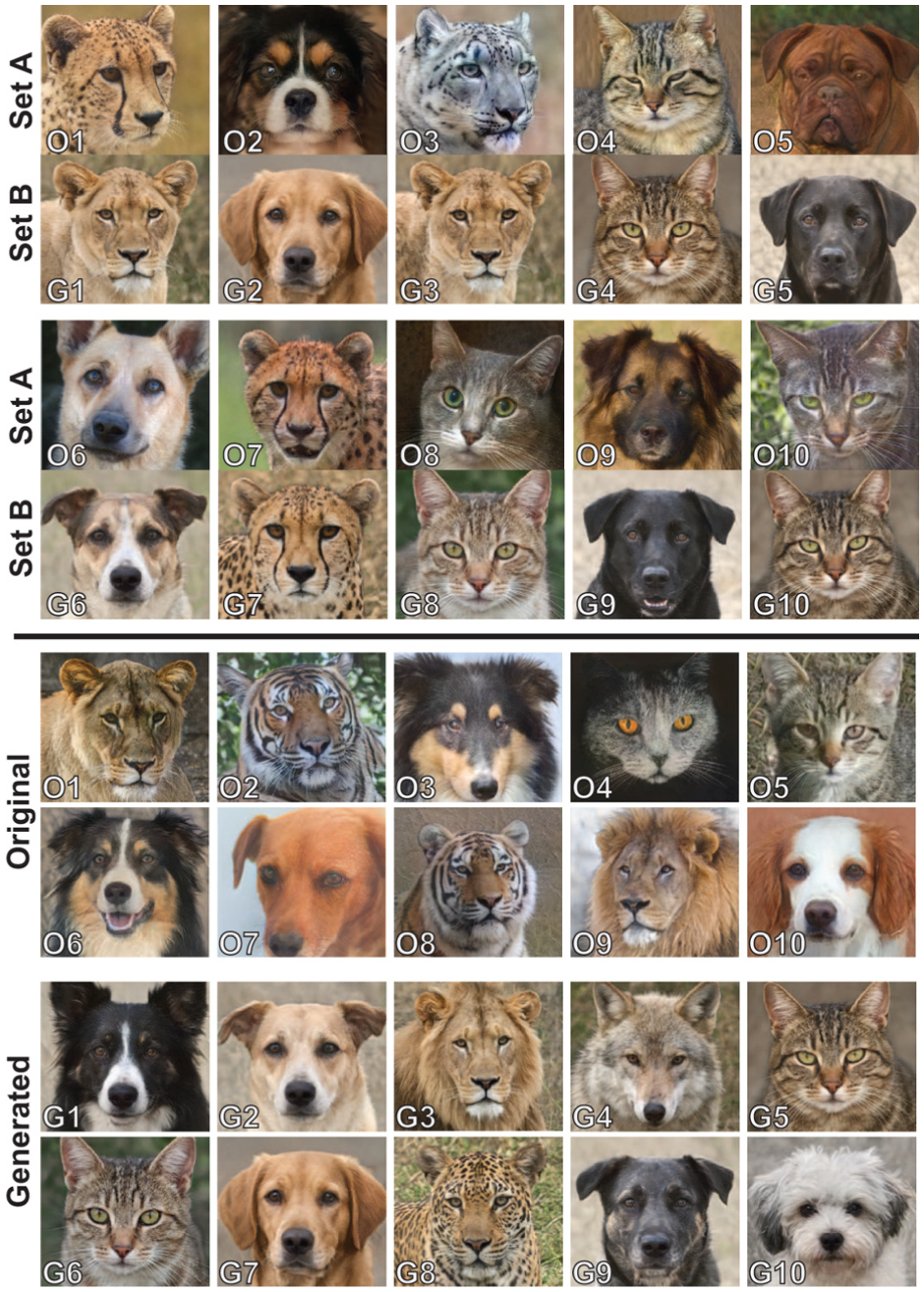
T1 Uniqueness: Participants were shown 10 images randomly picked from AFHQv2 (set A) and 10 images (set B) created by LCIP (fixed) applied to the original image’s location in the projection, see Figure 20 top. For each B image, participants were asked to choose the most similar image in A or reject all if none looked similar. Several B images can be assigned to one A image. T1 also helped participants to get to know the dataset as they were always informed if images were original or generated. We measured the uniqueness of generated images by aggregating participants’ choices – fewer associations indicating higher uniqueness.

Figure 20.

User evaluation. Top: 10 image pairs used for Task 1: Uniqueness. Bottom: 10 original images (O1–O10) and 10 generated images (G1–G10) used for Task 2: Fidelity.

Results: Images G6 and G7 were always assigned to the originals O6 and O7. G10 was assigned 11/15 times to the original O10 alongside G4 and G8. For O8, most users selected O8 itself as the most similar image. Most users reported they could easily find a similar image for most images; a few could not find one at all. Statistical analysis confirms this: Participants completed 150 matching trials with $k = 67$ correct assignments, yielding an observed accuracy $\bar{p} = 0.447$ . A one-sample $z$ -test against chance level ( $H_{0} : p = 0.1$ ) gives $z \approx 14.1$ ( $p << 0.0001$ ), so we reject $H_{0}$ and support $H_{1} : p > 0.1$ . The 95% confidence interval $[0.367, 0.526]$ is fully above 0.1, so participants performed 0.347 (34.7%) above chance.

Interpretation: LCIP (fixed), that is, without user control, could generate images that are assignable to a ground-truth image. However, this highly depends on the local variance of the data. This can be seen by users selecting 3–4 different images in some cases, while in others, they unanimously selected the same single image. While participants said that it was not easy to find a similar image, they assigned correct counterparts above chance; this supports the claim that LCIP can generate visually distinct images.

T2 fidelity: Participants were shown 20 images (Figure 20 bottom) and asked to tell whether each was original or generated. Ten images were randomly selected from AFHQv2; the other 10 were created by LCIP (fixed), sampled based on point density in the projection to ensure a representative set. By assessing one’s ability to distinguish between original and generated images, this task gauges the fidelity of LCIP.

Results: Most participants incorrectly classified most images: image G8 (13/15 original), image O3 (13/15 generated), and image G1 (12/15 original). Results for G3, G4 and G6 were close to a tie – 8/15 users marked these as original. Images O6 and G5 were correctly classified as original, respectively generated, by 10/15 users. Overall participants achieved only 39.67% accuracy, much below the 50% chance level. The 95% confidence interval $[0.342, 0.452]$ lies fully below 0.5. This leads us to reject the alternative hypothesis $H_{1} : p > 0.5$ and tells that participants were unable to reliably distinguish between original and generated images.

Interpretation: Users mentioned looking for artifacts in the images to tell whether they were generated or not. Some participants agreed when asked whether ‘normal’ imperfections in an image made them think it was generated, while the generated image generally looked clean and polished. Overall, results show that LCIP creates data which is hard to distinguish from true data.

T3 Smoothness (natural interpolation order): Participants were given a start and end image created using LCIP and 6 in-between interpolated images – see rows marked with rows in Figure 19(b–d, f, and G), yielding five trials for this task. Users were asked to arrange the interpolated images in the perceived correct order between the start and end images using paper printouts set on a table. The match between the participants’ order and the actual interpolation order was used to measure the smoothness and understandability of LCIP.

Results: Participants could recover the interpolation order at high rates: 11 (trial 1); 13 (trial 2); all (trial 3); all but one (trial 4); and 11 (trial 5). Participants reported that they found it easy to order the images. In cases with larger changes in the animal’s appearance, for example, fur color, participants mentioned using features like facial expressions or viewing directions to infer the order. For each trial $T_{j}$ , we compared the number of correctly ordered intermediate images with the chance baseline $μ_{chance} = 1$ (six intermediate images give a $1 / 6$ success probability). One-sample $t$ -tests strongly rejected $H_{0} : E [T_{j}] = μ_{chance}$ in favor of $H_{1} : E [T_{j}] > μ_{chance}$ ; even the weakest trial yielded $t \approx 12.9$ ( $p << 0.001$ ). Hence participants achieved significantly higher scores than chance.

Interpretation: Most users recovered LCIP’s interpolation order, telling that our method creates smooth transitions. Since users were particularly successful in trial 3, our results show that LCIP can create meaningful and smooth transitions between species (here, cat and fox).

T4 Controllability: Participants were introduced to the LCIP image-manipulation tool (Figure 1) by a free exploration phase. Next, they were asked to pick a dog image and modify it to make it smile using source image 2852 (a white laughing Samoyed) as reference; and next to do the same with a cat image.

Results: All users could transfer the smile in image 2852 to other dogs. Using the $α$ slider was found intuitive and easy – less so for the $σ$ slider. Users did not overall succeed in transferring the smile from the dog to a cat image, yet found that other cat features, for example, fur or viewing direction, got more similar to the dog image. Directly manipulating images to transfer styles like ‘sticking out the tongue’ was found useful by all participants (P1–P15). Transferring desired styles between different animal species consistently was found difficult (P1, P4, P7, P15). Participants first struggled to understand what the $α$ and $σ$ parameters actually mean; this improved with practice for over half of them (P2, P3, P7, P9, P11–P15). Critiques included insufficient labeling of parameters; improvements suggested adding more visual explanations of how parameters affect the high-dimensional data (P3, P7, P13, P14). The simple handling of sliders, showing changes visually, and ability to compare projections with original images were found helpful and functional (all participants except P1, P4 and P8). Some participants wished more precise controls to adjust image features such as fur color, eye shape, or body posture (P9, P12–P15). Overall, the ability to manipulate projections and visually track change effects were found exciting and useful (P10–P14).

Interpretation: Most T4 participants had positive impressions of LCIP’s ability to support style transfer and consistently managed to get the desired results for the dog image (less so for the cat image). Expectedly, learning to effectively use LCIP’s parameters to get the desired results took some effort. We should note that this task is quite challenging; its success depends not only on LCIP’s abilities but also on the used data – for example, if only a few smiling cat examples exist compared to dog ones, it is much harder for any interpolator to transfer a smile style from a dog to a cat.

Discussion

We next discuss several aspects of our method.

Controllability: To our knowledge, LCIP is the first user-controlled inverse projection that breaks the limitation that inverse projections land on a surface embedded in $n$ D (section ‘Controllability: Going beyond a fixed surface’). LCIP allows this inversely-projected surface to be put anywhere and smoothly adjusted (section ‘Smoothness of controlled inverse projections’ and Task 3 in section ‘User study: Evaluating LCIP in practice’). Related to this point, we also note the differences between LCIP and other data augmentation or interpolation techniques such as SMOTE⁵²: While all inverse projections do data augmentation by construction, classical data augmentation works purely in data space, driven by structural or statistical properties of the dataset to be enriched. In contrast, inverse projections (like ours but not only) enrich a dataset in a controlled way – the added points must map to 2D locations in the embedded (projection) space. This allows one to actually explore the (enriched) data space by exploring the 2D projection space.

Genericity: We demonstrated LCIP with image style-transfer as this is an illustrative application for inverse projections. Yet, LCIP is not limited to image data, as shown by the controllable decision maps example in section ‘Controllability: Going beyond a fixed surface’; nor should it be seen as competing with dedicated image-style-transfer methods. Our method can control inverse projections created by any user-selected projection $P (X)$ of any high-dimensional dataset $X$ . On the other hand, the practical application of LCIP – or, for that matter, any other inverse projection – to explore a high-dimensional data space works easiest when the data are directly displayable, for example, for images or 3D shapes.¹⁸ If data were abstract feature vectors obtained by for example, an autoencoder, or samples of a time series, LCIP (or other inverse projections) would technically work equally well but user control of the inverse projection would be less intuitive. This is not a problem of inverse projections but of how to intuitively display high-dimensional data samples in a 2D projection space. How to do this effectively for non-visual data e.g. audio data or general-purpose feature data is an open problem for future research.

Quality: Our evaluations show that LCIP has higher quality in gap areas than existing inverse projection techniques (section ‘Comparison to other inverse projection methods’). Also, LCIP creates smoother-varying data samples (when its 2D input changes smoothly). The user study (section ‘User study: Evaluating LCIP in practice’) further confirmed the uniqueness, fidelity, and smoothness of LCIP. Smoothness is of key added value in user-driven applications; non-smooth inverse projections would cause difficulty and confusion for users who aim to control how 2D points are backprojected to the data space.

Scalability: LCIP’s speed is linear in the number of inversely projected points and, in practice, similar to state-of-the-art inverse projection methods, for example, NNinv (section ‘Gradient maps for the tested inverse projections for UMAP on MNIST’).

Projection: We tested LCIP using two projection methods, t-SNE and UMAP, as these methods consistently score high projection quality metrics for datasets of varying (intrinsic) dimensionality and of different provenances,¹³ making them prevalent methods in visualization and visual analytics. This means that the 2D scatterplots that t-SNE and UMAP create allow an easier exploration by users than those from a lower-quality $P$ . In turn, this makes the information lost during projection to be lower than when using a low-quality $P$ , which makes LCIP’s interactive control easier. Yet, for specific datasets, other techniques than t-SNE or UMAP could yield higher quality and thus be preferable as basis for LCIP. LCIP can handle any $P$ in a fully black-box manner, so using other techniques can be directly done when desired.

Ease of use: To inversely project a source point, LCIP needs minimally only selecting that point in the 2D projection space. To modify the inverse projection, one needs also to select one target point (from the projected ones) and a ‘pull’ factor $α$ telling how much the source will change towards the target. Such operations are simple to perform in a GUI by clicking (to select points) and pulling a slider (to change $α$ ). Users can also change how smooth the inverse projection is around a source point by changing $σ$ – again, just by pulling a slider.

Generalization: Three levels of generalization exist for both direct and inverse projections $M$ : (1) Transductive: $M$ can handle a given dataset but needs re-training from scratch when data changes (e.g. t-SNE). (2) Out-of-sample: $M$ can handle without retraining any dataset drawn from the same distribution as its training data (e.g. UMAP, NNP, and all the inverse projection methods mentioned in this article, including LCIP). (3) Cross-domain inductive: $M$ can handle without retraining data drawn from different domains. No direct or inverse projection method we are aware of attains type 3 flexibility. In particular, for inverse projections, this would mean building a single model which can output data of different dimensionalities without retraining or changing model architecture. This is a significant challenge which we leave for future work.

Limitations: LCIP disentangles the information captured by a projection $P$ from what $P$ cannot capture, and next manipulates this information to control the inverse projection. We argued that this makes good sense technically. Yet, from a practical viewpoint, as T4 in section ‘User study: Evaluating LCIP in practice’ also shows, it is by far not clear for a user what a given $P$ would capture (and thus not under user control) and what is, thus, controllable. Our experiments showed that, for selected datasets, the projection captures the core similarity of items, while the lost information – under user control – mainly affects a generic attribute we called ‘style’. Yet, what exactly style is; how it differs from what a given projection captures; and how much style is controllable in practice, are questions that we cannot formally answer for all datasets and all projection methods. Separately, LCIP is limited to the convex hull of samples in $X$ . As shown in Task 4 in section ‘User study: Evaluating LCIP in practice’, transferring the ‘sticking out tongue’ style from a dog to a cat image is generally not successful, likely due to this combination falling outside of the said hull. Exploring how to make $P^{- 1}$ go beyond this convex-hull space is a valid option to investigate. Finally, while our examples of style transfer on images are, we hope, convincing evidence for LCIP’s abilities, more use-cases are needed to strengthen our claims of added value of controllable inverse projections.

Conclusion

We have presented an inverse projection method that allows users to break the barrier of creating two-dimensional, fixed, surfaces embedded in the data space – a property exhibited by all inverse projection methods we are aware of. To do this, we split the information present in the high-dimensional data into (1) information captured by a projection technique and (2) a latent code, namely, information that such a technique cannot capture. Next, we allow users to interactively control this latent code and thereby generate a dynamic inverse projection which can effectively ‘sweep’ the data space between the samples used by the direct projection it aims to invert.

Several experiments show that our method meets a number of key requirements for inverse projections: Our method is – in absence of user control – at least as accurate, and as computationally scalable, as state-of-the-art inverse projection techniques. When user control is added, our method enables users to specify where the inverse projection should adapt to so-called target data points, and where the underlying direct projection should purely drive it. This control is simple to perform as it involves changing two linear parameters – an action radius and an action amount. The data points generated by our method change smoothly as the control parameters change – which is desirable from a practical perspective. Also, we showed that our method can cover a larger area of the data space – measured in terms of intrinsic dimensionality – than other inverse projection methods. Last but not least, we showed that our inverse projection method creates data samples (images in our studies) that look more natural than those created by existing inverse projection methods.

LCIP could be used next to assist user-controlled 3D shape morphing¹⁸– its control would directly allow users to select specific target shapes to use during the morphing. Separately, LCIP can help data augmentation by e.g. subsampling a dataset to be augmented to get the sources; hand-picking specific samples (having e.g. different styles) as targets; and creating the desired number of augmented samples by our interpolation. Smart sampling strategies like SADIRE⁵³ can be used both to highlight samples in the projection scatterplot which are interesting for users to explore or manipulate first via LCIP; and also, potentially, to fine-tune LCIP’s training by adding extra weights to such samples. We also plan to make LCIP’s control more intuitive by displaying the kind of information that is captured by our latent codes, thereby showing users what they would control when manipulating LCIP’s parameters. Finally, we plan to refine LCIP’s local control of decision maps (section ‘Controllability: Going beyond a fixed surface’) to allow analysts to explore trained models around regions of interest in simpler, but more effective, ways.

Supplemental Material

sj-pdf-1-ivi-10.1177_14738716261455130 – Supplemental material for LCIP: Loss-controlled inverse projection of high-dimensional image data

Supplemental material, sj-pdf-1-ivi-10.1177_14738716261455130 for LCIP: Loss-controlled inverse projection of high-dimensional image data by Yu Wang, Frederik L. Dennig, Michael Behrisch and Alexandru Telea in Information Visualization

Footnotes

ORCID iD

Yu Wang

Author contributions

Yu Wang: Conceptualization, Methodology, Software, Investigation, Formal analysis, Visualization, Data curation, Writing – original draft. Frederik L. Dennig: User study design and execution, User study analysis, Writing – review and editing. Michael Behrisch: Writing – review and editing. Alexandru Telea: Conceptualization, Supervision, Writing – review and editing.

Funding

The authors received no financial support for the research, authorship, and/or publication of this article.

Declaration of conflicting interests

The authors declared no potential conflicts of interest with respect to the research, authorship, and/or publication of this article.

Supplemental material

Supplemental material for this article is available online.

References

Lespinats

Aupetit

. CheckViz: sanity check and topological clues for linear and nonlinear mappings. Comput Graph Forum 2011; 30(1): 113–125.

Sorzano

COS

Vargas

Montano

. A survey of dimensionality reduction techniques. arXiv, arXiv:1403.2877, 2014.

Nonato

Aupetit

. Multidimensional projection for visual analytics: linking techniques with distortions, tasks, and layout enrichment. IEEE TVCG 2018; 25: 2650–2673.

Rodrigues

FCM

. Visual analytics for machine learning. PhD Thesis, University of Groningen, 2020.

Benato

Grosu

Falcão

, et al. Human-in-the-loop: using classifier decision boundary maps to improve pseudo labels. Comput Graph 2024; 124: 104062.

Rodrigues

FCM

Espadoto

Hirata

, et al. Constructing and visualizing high-quality classifier decision boundary maps. Information 2019; 10(9): 280.

Oliveira

Espadoto

Hirata

Jr , et al. SDBM: supervised decision boundary maps for machine learning classifiers. In: Proceedings of the international conference on information visualization theory and applications, Algarve, Portugal, 5–7 March, 2011, pp. 77–87.

Schulz

Hinder

Hammer

. DeepView: visualizing classification boundaries of deep neural networks as scatter plots using discriminative dimensionality reduction. In: Proceedings of the thirty-fourth international joint conference on Artificial Intelligence, Montreal, QC, Canada, 16–22 August 2025, pp. 2305–2311.

Amorim

Brazil

Daniels

, et al. iLAMP: exploring high-dimensional spacing through backward multidimensional projection. In: Proceedings of the IEEE symposium (or conference) on visual analytics science and technology, Vienna, Austria, 3 November 2025, pp. 53–62.

10.

Espadoto

Appleby

Suh

, et al. UnProjection: leveraging inverse-projections for visual analytics of high-dimensional data. IEEE TVCG 2021; 29(2): 1559–1572.

11.

Machado

Behrisch

Telea

. Exploring classifiers with differentiable decision boundary maps. Comput Graph Forum 2024; 43(3): e15109.

12.

Zheng

Shen

Yang

, et al. Autoencoders with intrinsic dimension constraints for learning low dimensional image representations. arXiv. arXiv:2304.07686, 2023.

13.

Espadoto

Martins

Kerren

, et al. Toward a quantitative survey of dimension reduction techniques. IEEE TVCG 2019; 27(3): 2153–2173.

14.

Wang

Telea

. Fundamental limitations of inverse projections and decision maps. In: Proceedings of the 19th International Joint Conference on Computer Vision, Imaging and Computer Graphics Theory and Applications (VISIGRAPP 2024), Vol. 1, Rome, Italy, 27–29 February 2024, pp. 571–582. SCITEPRESS.

15.

Van der Maaten

Hinton

. Visualizing data using t-SNE. J Mach Learn Res 2008; 9(11): 2579–2605.

16.

McInnes

Healy

Melville

. UMAP: uniform manifold approximation and projection for dimension reduction. arXiv. arXiv:1802.03426, 2018.

17.

Joia

Coimbra

Cuminato

, et al. Local affine multidimensional projection. IEEE TVCG 2011; 17(12): 2563–2571.

18.

Amorim

Vital Brazil

Mena-Chalco

, et al. Facing the high-dimensions: inverse projection with radial basis functions. Comput Graph 2015; 48: 35–47.

19.

Espadoto

Hirata

Telea

. Self-supervised dimensionality reduction with neural networks and pseudo-labeling. In: Proceedings of the international conference on information visualization theory and applications, Algarve, Portugal, 5–7 March, 2011. SciTePress, pp. 27–37.

20.

Hinton

Salakhutdinov

. Reducing the dimensionality of data with neural networks. Science 2006; 313(5786): 504–507.

21.

Blumberg

Wang

Telea

, et al. Inverting multidimensional scaling projections using data point multilateration. In: Proceedings of the 15th International EuroVis Workshop on Visual Analytics (EuroVA), Odense, Denmark, 27 May 2024. The Eurographics Association.

22.

Torgerson

. Multidimensional scaling: I. Theory and method. Psychometrika 1952; 17: 401–419.

23.

Kruskal

. Multidimensional scaling by optimizing goodness of fit to a nonmetric hypothesis. Psychometrika 1964; 29(1): 1–27.

24.

Espadoto

Rodrigues

Hirata

NST

, et al. Deep learning inverse multidimensional projections. In: Proceedings of the 10th International EuroVis Workshop on Visual Analytics (EuroVA), Porto, Portugal, 3 June 2019, pp. 13–17. The Eurographics Association.

25.

Dennig

Geyer

Blumberg

, et al. Evaluating autoencoders for parametric and invertible multidimensional projections. In: Proceedings of the 16th International EuroVis Workshop on Visual Analytics (EuroVA), Luxembourg, 2 June 2025. The Eurographics Association.

26.

Wang

Machado

Telea

. Quantitative and qualitative comparison of decision map techniques for explaining classification models. Algorithms 2023; 16(9): 438.

27.

Ansuini

Laio

Macke

, et al. Intrinsic dimension of data representations in deep neural networks. In: Advances in Neural Information Processing Systems 32 (NeurIPS 2019), Vancouver, BC, Canada, 8–14 December 2019, pp. 6109–6119. Curran Associates, Inc.

28.

Wang

Yao

Zhao

. Auto-encoder based dimensionality reduction. Neurocomputing 2016; 184: 232–242.

29.

Marin

Gotovac

Russo

, et al. The effect of latent space dimension on the quality of synthesized human face images. J Comm Softw Sys 2021; 17(2): 124–133.

30.

Padala

Das

Gujar

. Effect of input noise dimension in GANs. In: Neural information processing. Lecture notes in computer science. Springer, pp. 558–569.

31.

Moyer

Gao

Brekelmans

, et al. Invariant representations without adversarial training. In: Advances in Neural Information Processing Systems 31 (NeurIPS 2018), Montréal, Canada, 3–8 December 2018, pp. 9084–9093. Curran Associates, Inc.

32.

Hadad

Wolf

Shahar

. A two-step disentanglement method. In: Proc., IEEE/CVF Conference on Computer Vision and Pattern Recognition (CVPR), Salt Lake City, UT, USA, 18–22 June 2018, pp. 772–780. IEEE.

33.

Mathieu

Zhao

, et al. Disentangling factors of variation in deep representation using adversarial training. In: Advances in Neural Information Processing Systems 29 (NIPS 2016), Barcelona, Spain, 5–10 December 2016, pp. 5041–5049. Curran Associates, Inc.

34.

Xie

Dai

, et al. Controllable invariance through adversarial feature learning. In: NIPS’17: proceedings of the 31st international conference on neural information processing systems, Long Beach, CA, USA, 4–9 December 2017.

35.

Jaiswal

AbdAlmageed

, et al. Unified adversarial invariance. arXiv, arXiv:1905.03629, 2019.

36.

Zheng

Sun

. Disentangling latent space for VAE by label relevant/irrelevant dimensions. In: Proceedings of the IEEE/CVF Conference on Computer Vision and Pattern Recognition (CVPR), Long Beach, CA, USA, 16–20 June 2019, pp. 12192–12201. IEEE.

37.

Goodfellow

Pouget-Abadie

Mirza

, et al. Generative adversarial networks. arXiv, arXiv:1406.2661, 2014.

38.

Pan

Tewari

Leimkühler

, et al. Drag Your GAN: interactive point-based manipulation on the generative image manifold. arXiv, arXiv:2305.10973, 2023.

39.

Karras

Laine

Aittala

, et al. Analyzing and improving the image quality of StyleGAN. arXiv, arXiv:1912.04958, 2020.

40.

Espadoto

Hirata

NST

Telea

. Deep learning multidimensional projections. Inf Vis 2020; 19(3): 247–269.

41.

Paszke

Gross

Massa

, et al. PyTorch: an imperative style, high-performance deep learning library. arXiv, arXiv:1912.01703, 2019.

42.

Wang

Dennig

Behrisch

, et al. LCIP implementation source code, https://github.com/wuyuyu1024/lcip.git (2025).

43.

LeCun

Cortes

Burges

. MNIST handwritten digit database, http://yann.lecun.com/exdb/mnist (2010, accessed 1 June 2023).

44.

Xiao

Rasul

Vollgraf

. Fashion-MNIST: a novel image dataset for benchmarking machine learning algorithms. arXiv, arXiv:1708.07747, 2017.

45.

Anguita

Ghio

Oneto

, et al. Human activity recognition on smartphones using a multiclass hardware-friendly support vector machine. In: Proceedings of the third international workshop on ambient assisted living, Vitoria-Gasteiz, Spain, 3–5 December 2012, pp. 216–223.

46.

Choi

Yoo

, et al. StarGAN v2: diverse image synthesis for multiple domains. In: Proceedings of the IEEE/CVF Conference on Computer Vision and Pattern Recognition (CVPR), 2019, pp. 8185–8194. IEEE.

47.

Jaiswal

Abd-Almageed

, et al. Unsupervised adversarial invariance. In Advances in Neural Information Processing Systems 31 (NeurIPS 2018), Montréal, Canada, 3–8 December 2018, pp. 5097–5107. Curran Associates, Inc.

48.

Tian

Zhai

, Van Driel D et al. Using multiple attribute-based explanations of multidimensional projections to explore high-dimensional data. Comput Graph 2021; 98: 93–104.

49.

Chatzimparmpas

Martins

Kerren

. t-viSNE: interactive assessment and interpretation of t-SNE projections. IEEE TVCG 2020; 26(8): 2696–2714.

50.

Venna

Kaski

. Visualizing gene interaction graphs with local multidimensional scaling. In: Proceedings of ESANN’06, 14th European Symposium on Artificial Neural Networks, Bruges, Belgium, 26–28 April 2006, pp. 557–562. d-side group.

51.

Venna

Peltonen

Nybo

, et al. Information retrieval perspective to nonlinear dimensionality reduction for data visualization. J Mach Learn Res 2010; 11: 451–490.

52.

Chawla

Bowyer

Hall

, et al. SMOTE: synthetic minority over-sampling technique. J Artif Intell Res 2002; 16(1): 321–357.

53.

Marcilio-Jr

Eler

. SADIRE: a context-preserving sampling technique for dimensionality reduction visualizations. J Visual 2020; 23: 999–1013.

Supplementary Material

Please find the following supplemental material available below.

For Open Access articles published under a Creative Commons License, all supplemental material carries the same license as the article it is associated with.

For non-Open Access articles published, all supplemental material carries a non-exclusive license, and permission requests for re-use of supplemental material or any part of supplemental material shall be sent directly to the copyright owner as specified in the copyright notice associated with the article.

8.98 MB

0.00 MB