A fast ray casting method for sound refraction at shear layers

Abstract

The application of microphone arrays for aeroacoustic measurements in wind tunnels with an open test section requires to consider the sound refraction at the shear layer. Several methods are available for this that are either applicable to special scenarios such as planar or cylindrical thin shear layers or that require considerable computational effort. The paper concerns a new method for general application—ray casting—that is based on a ray tracing method. Ray tracing is briefly revisited and it is shown that the computational effort becomes quite high especially for large mapping grids. The ray casting approach with its interpolation technique is introduced. A time reversal technique is the key to make this approach very efficient and fast. Finally, the approach is demonstrated using two example results from simulation and from a practical measurement.

Keywords

Ray tracing sound refraction microphone array

Introduction

A number of different methods are available for the application of microphone arrays to the characterization of aeroacoustic sources. Regardless of their specific approach all these methods require a model for the sound propagation from the sound sources to the individual microphones of the array. The quality of this propagation model finally determines also the quality of the measurement results. In a case with no flow present and a homogeneous medium bearing the sound, this model is simply based on the free field Green’s function.

However, many practical applications require a more sophisticated approach. One example would be an open jet wind tunnel where the microphones are mounted outside of the flow while the sources are located within the jet. In this case, the sound must propagate through the shear layer separating the jet from the quiescent surrounding in order to arrive at the microphones. On its way the sound is convected by the flow. In addition, it refracts at the shear layer. Thus, the travel times from source to microphone are affected. Compared to the case of no flow, these times may be shorter or longer. Moreover, the amplitude of sound arriving at the microphone is also altered.

A propagation model for microphone array measurements must therefore consider these effects. Generally, there are three options to account for the refraction at a shear layer in the model. They are quite different with respect to how they treat the shear layer flow field and the propagation of sound.

The first possibility is to model the shear layer as an infinitely thin vortex sheet separating two regions of homogeneous flow with different flow speeds (one could be equal to zero). The method of Amiet¹ and some later improvements² handle the refraction at such shear layer of simple geometry like a plane or a cylindrical surface. While being computationally inexpensive, these methods cannot handle thicker shear layers. Moreover, the handling of arbitrary jet geometries is difficult.

A second option is to solve some form of wave equation or general model for sound propagation in flows. For arbitrary flows, this can be done using numerical approaches to the computation of the sound field such as the finite element method (FEM)³ or by the application of a suitable computational aeroacoustics (CAA) method^4–6 that computes sound propagation. These methods yield results of high accuracy. However, instead of only the required information regarding the propagation from source to microphones, the whole sound field is computed at the expense of relatively high computational cost.

The third approach relies on the tracing of sound ‘rays’ through the flow field. A variety of ray tracing approaches (e.g. see literature^7–11) suitable for inhomogeneous flows are available in the context of geometrical acoustics. They require to integrate a system of differential equations in order to trace a ray through a possibly inhomogeneous medium with arbitrary flow. Without the need to compute the whole sound field, these methods need considerably less computational resources than FEM or CAA methods. They offer better accuracy but are computationally more expensive than vortex sheet methods.

In a typical application of a microphone array in an aeroacoustic wind tunnel, the sound sources are mapped onto a grid of possible sound sources. Thus, it is necessary to estimate sound propagation from M locations of possible sound sources in the grid to N locations of microphones. This means that altogether $N$ individual travel times have to be computed. In Figure 1 an example¹² is shown that concerns the analysis of airfoil noise. Two options for the mapping grid are considered. The first option is a two-dimensional grid as it is traditionally used. It contains M = 3721 possible source locations. The second option is a three-dimensional grid which is desirable in some cases with $M = 226, 981$ . The number of microphones in the example is 56, so that $2 \cdot 10^{5}$ (2D) and $1.3 \cdot 10^{7}$ (3D) travel times have to be computed.

Figure 1.

Typical application: two-dimensional (blue) or three-dimensional grid (green) for the mapping of sources at an airfoil in an open jet wind tunnel using a microphone array (red), grids thinned for clarity by factor 4.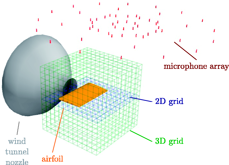

These high numbers require an efficient computational method, otherwise the computation would last for an unacceptably long time. For the first option, thin vortex sheet methods, it can be assumed that the computation is sufficiently fast. The second option would require considerable computational effort because the FEM or CAA model has to be solved at least several thousand times. This probably renders its use impracticable. The third option, ray tracing, is more accurate than the first, but possibly faster than the second.

Thus, the present contribution focuses on ray tracing to compute sound propagation in the context of microphone array application to aeroacoustic source characterization. First, the theory of ray propagation is shortly reviewed and the numerical procedure of tracing a single ray is discussed. Then, an interpolation method is introduced that renders the simultaneous computation of sound propagation to many microphone positions much more efficient. Afterward, it is discussed how a simple time reversal strategy minimizes the necessary computational effort. Finally, some implementation details are explained and example results are given.

Ray tracing

During the propagation in a quiescent homogeneous medium, the sound does not change its direction of propagation. If the sound originates from a point source, then the sound that was generated at a certain time will later pass through a spherical surface where every point on that surface receives the sound at the same instant t. Thus, the surface is called a wavefront.

If there is an inhomogeneous flow field with a velocity $v (x, t)$ that depends on the location x and a possibly variable speed of sound $c (x)$ , the wavefront is no longer a spherical surface, but has an arbitrary form, implicitly given by $τ (x) = t$ . For a different instant t there is a different wavefront. This can be understood as a movement of the wavefront. If $x_{p}$ is a point on the wavefront, then it moves along with the wavefront at the speed given by¹⁰

\frac{d x_{p}}{dt} = v (x_{p}, t) + n (x_{p}, t) c (x_{p})

(1)

where

n (x_{p}, t)

is the unit normal vector describing the wavefront. The trajectory of the movement of

x_{p}

can be seen as a ray of sound. In order to find out about the propagation of sound, this ray has to be traced.

For the ray tracing using equation (1) the wavefront normal needs to be known. Alternatively, the “wave slowness” $s = \nabla τ$ can be used, which is a vector that is also normal to the wavefront, but with a magnitude which is the inverse of the speed the wavefront itself is moving. It is given by

s (x, t) = \frac{n (x, t)}{c + v (x, t) \cdot n (x, t)}

(2)

If n is now replaced by $\frac{s}{| s |}$ , then s is still needed to do the ray tracing. From the temporal change of the wave slowness along the ray

\frac{d s (x_{p})}{dt} = (\frac{\partial x_{p}}{\partial t} \cdot \nabla) s (x_{p})

(3)

and equation (2) an additional differential equation for the wave slowness can be constructed that complements the first differential equation (1).

Both differential equations can be written as a system of ordinary differential equations (ODE) in Cartesian co-ordinates (i = 1, 2, 3)

\frac{{dx}_{i} (t)}{dt} = \frac{{cs}_{i} (t)}{| s (x, t) |} + v_{i} (x, t)

(4)

\frac{{ds}_{i} (x (t), t)}{dt} = | s (x, t) | \frac{\partial c}{\partial x_{i}} + \sum_{j = 1}^{3} s_{j} (x, t) \frac{\partial v_{j} (x, t)}{\partial x_{i}}

(5)

where

x (t)

is now the ray trajectory. For the shear layer refraction problem at hand, we may assume that the velocity field is not time dependent and it is sufficient to look only at the space-dependent mean velocity

v (x)

. Moreover, in many practical cases temperature effects on the speed of sound are negligible so that c can be assumed to be a constant. The time t is the ray travel time and for the application at hand it is the ultimate goal to estimate this travel time for a ray from source to microphone.

Given a start location $x (t_{0})$ and a wavefront normal $n (t_{0})$ , the system (4) and (5) can be integrated to trace the ray. This will also produce the travel time from $x (t_{0})$ to any location along the ray. However, it is not possible to know a priori which locations the ray will pass through. Consequently, in order to calculate the travel time t_R for a ray between a source at $x (t_{0})$ and a microphone at $x (t_{R})$ , first a particular ray passing through the microphone position needs to be found. This is no longer an initial value problem, but a boundary value problem which needs to be solved using a shooting method. Within an iterative algorithm, the ODE system is then repeatedly integrated with different starting conditions until the solution ray hits the microphone.

One possible implementation of this approach using an implicit Adams method for ODE integration and a derivative-free Nelder–Mead method to minimize the distance between ray and the microphone needs about 200 rays to hit the target. This results in a computation time of about 0.5–1 s per source–microphone pair which is acceptable if only a few of such computations are to be made. In the typical application case, this means several days for the two-dimensional grid and as much as four months for the three-dimensional grid. Even when using a faster implementation, the computation times are unacceptably long for practical applications.

Ray casting and spatial interpolation

While the tracing of a single ray may be adequate in the general case, the application to microphone array measurements allows some special assumptions that can enable a more efficient approach to compute all the required travel times between each source–microphone pair. A first helpful assumption that can be made is that the microphones are not located in the jet directly upstream a source. Thus, the rays that are emitted from one source and finally hit one of the microphones are not subject to a total reflection at the shear layer. Further, at least for practically relevant cases of flows that are not excessively curved in the flow direction, the wavefront toward the microphones can be assumed to be convex. This means that no ray hitting a microphone intersects there with other rays from the same source. Thus, there is only one unique travel time for each source–microphone pair.

The second assumption concerns the differences between travel times for different microphones but the same source. If the microphones are close to each other, then the travel times are not very different. Thus, if the travel time from one source is treated as a function of the microphone location, this function is relatively smooth (see also the examples in “Results” section). A smooth function is a good candidate for interpolation. Values of such a function can be interpolated from individual function values.

In case of the travel time $t_{R} (x)$ , for a spatial interpolation it is sufficient to know the values at the nodes of a three-dimensional mesh. This mesh can be produced by a bunch of rays originating from the same source, but starting in different evenly distributed directions (ray casting). Each of these rays has to be traced by integrating the ODE system (4) and (5). Temporal sampling along these rays gives locations and assigned travel times. Thus, these samples can be treated as the nodes of the mesh. From these nodes, a tetrahedral mesh can be constructed using Delaunay triangulation. Within each tetrahedral mesh cell, $t_{R} (x)$ can be interpolated from the four nodal values using linear barycentric interpolation.

This straightforward approach allows to quickly compute the travel time to any location within the mesh, while this is not possible for locations outside the mesh. In order to compute the travel times for the microphones in the array, all microphone locations have to be inside the mesh region. To ensure this, the start directions of the rays casted must cover a sufficient solid angle and the tracing of each ray must continue long enough to cover the required distance between the source and all microphones.

This ray casting approach can be implemented using the same ODE integration method as for the single ray. If about 200 rays are cast, then the computation time for each source is somewhat above 1 s. The number of microphones has nearly no influence on that computation time. For the typical example given in the “Introduction” section, the overall computation time for M repetitions of this approach is reduced to about 1 h for the two-dimensional grid and two days for the three-dimensional grid. This corresponds to a 50-fold reduction compared to the shooting method approach.

While these computation times can be handled in a practical application, a further reduction is possible based on the fact that the number of microphones is usually smaller than the number of source mapping grid points. Instead of tracing the ray from source to microphone, it is also possible to trace the ray backward from microphone to source using the concept of time reversal. The approach is exactly the same as for the source-to-microphone ray casting except that the velocity field must be reversed in time. This can easily be done by using $- v (x)$ instead of $v (x)$ and negative Jacobian of v instead of the Jacobian in the ODE system. Consequently, only N repetitions of the ray casting are required regardless of the grid dimensionality. Thus, the overall computation time is drastically reduced to about 100 s for both the two-dimensional and the three-dimensional case. This is definitely adequate.

Results

Simulation: Three monopole sources

The approach is first demonstrated here for the synthetic case of three monopole sources. In this scenario, three sources of same source strength are located within a round jet and emit incoherent white noise signals. A microphone array with 64 microphones arranged in seven logarithmic spiral arms outside of the jet flow receives the signals (Figure 2). At the nozzle exit, the jet has a diameter of $D_{0} = 0.5$ m and a flow speed of $U_{0} = 68.8$ m/s (M = 0.2). The microphone array has an aperture of 1.5 m and its plane is 0.5 m away from the jet axis. All three sources are located 0.6 m downstream from the nozzle while the array center is 0.5 m downstream from the nozzle. With the co-ordinate origin at the center of the array and the z-axis pointing toward the jet, the sources are located at x = 0.1 m, $y = {0, 0.12, 0.24}$ m, and z = 0.5 m. The jet axis is pointing in the positive x-direction.

Figure 2.

Three monopole sources in an open round jet with a microphone array outside of the jet.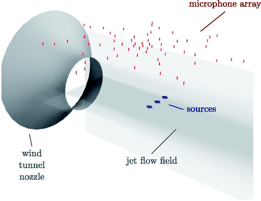

Because the shear layer is approximately halfway between sources and array, it can be expected that there is a more distinct effect on the sound travel times than for cases where either the shear layer is closer to the sources or closer to the array. Moreover, two of the sources are located off the jet axis which leads to ray paths inclined in different directions.

The jet flow is approximated as an isothermal jet. It is assumed that only the zone of jet flow establishment is of interest. An approximation for the flow in this zone is given in Albertson et al.,¹³ where a cylindrical co-ordinate system with co-ordinates x, r and the origin at the nozzle exit-plane center is used. The zone of flow establishment ( $0 < x < 6.2 D_{0}$ ) is characterized by a cone-shaped jet core with constant velocity

U_{x} = U_{0}, for r \leq \frac{D_{0}}{2} (1 - \frac{x}{6.2 D_{0}})

(6)

and a shear layer that represents the transition to the quiescent surrounding of the jet. The mean flow velocity within the shear layer is given by

U_{x} (x, r) = U_{0} \exp (- \frac{(r + C_{2} x - D_{0} / 2)^{2}}{2 (C_{2} x)^{2}}) with C_{2} = 0.081

(7)

In this model, entrainment velocity components are neglected, i.e. $U_{r} = U_{y} = U_{z} = 0$ . Figure 3 shows the flow field within the co-ordinate system of the array and source scene.

Figure 3.

Flow field in the jet having cylindrical symmetry, dashed line: shear layer.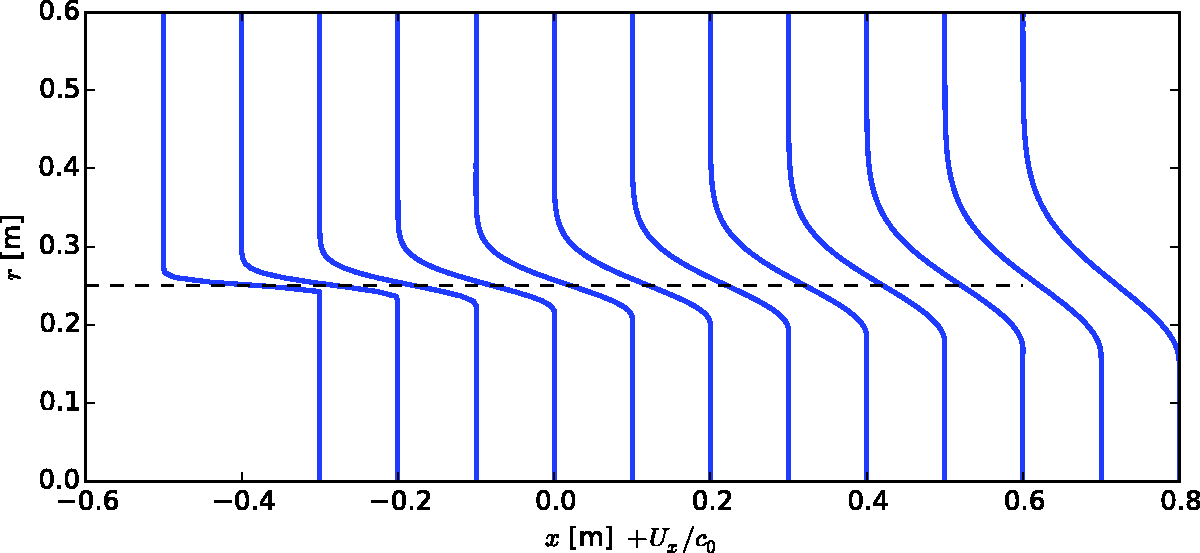

The ray casting approach is implemented as part of the open source microphone array signal processing library Acoular.¹⁴ For each microphone a bunch of rays pointing to the grid of possible source positions is generated. The ray density is given by the number N of rays per half-space solid angle $Ω = 2 π$ . The spatial distribution of the rays is calculated from directions ( $φ, θ$ ) given by a three-dimensional spiral on a spherical surface

h = - 1 + \frac{2 n}{2 N - 1}, n = 1, \dots, N

(8)

θ_{n} = \arccos (h)

(9)

φ_{0} = 0

(10)

φ_{i + 1} = (φ_{i} + \frac{3.6}{2 N (1 - h_{i + 1}^{2})}) 2 π

(11)

These ( $φ, θ$ ) directions need to be rotated so that the pole of the half sphere points to the grid center. The required maximum ray length l_max is assessed, and each ray is integrated using an implicit Adams method¹⁵ with a maximum step length of $10^{- 4} l_{\max}$ . Along the ray, approximately $\sqrt{N}$ positions and travel times are stored. From these data, the interpolating mesh is constructed using Delaunay triangulation.

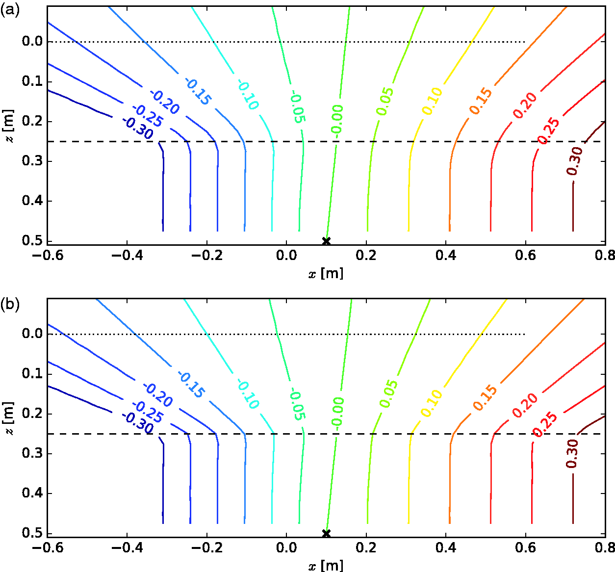
As a result from the ray casting approach, Figure 4 shows the wavefronts from source 0 at (0.1,0.0,0.5) m, given within the y = 0 plane and in the general direction toward the array. The influence of the shear layer is particularly apparent where the wavefront deviates from a spherical shape. Results assuming a “thick” shear layer (6) and (7) in Figure 4(a) are compared to results computed with the assumption of a thin shear layer around a cylindrical jet core in Figure 4(b). The differences between both cases are barely noticeable. They become more apparent, if instead of the wavefronts the difference between the sound travel times without and with jet flow is plotted. Figure 5 shows such plots and it becomes clear that there is indeed a subtle difference. Figure 6 shows the sound travel time between source 0 and locations in the array plane at y = 0 and z = 0. Again, the differences between the thick and the thin shear layer assumption appear to be very small. However, the difference between travel times without and with flow considered is obvious.

Figure 4.

Sound travel times from source 0 (×), given in milliseconds, dashed line: shear layer, dotted line: microphone array plane, gray: some ray paths. (a) Thick shear layer and (b) thin shear layer.

Figure 5.

Difference $Δ t_{0} - Δ t$ of sound travel times without flow ( $Δ t_{0}$ ) and with flow ( $Δ t$ ), from source 0 (×), given in milliseconds, dashed line: shear layer, dotted line: microphone array plane. (a) Thick shear layer and (b) thin shear layer.

Figure 6.

Sound travel time between source 0 and locations in the array plane at y = 0 and z = 0 for the case of no flow, jet with thick and with thin shear layer.

One important element of the ray casting approach is the interpolation within the mesh constructed by the rays. It can be expected that this interpolation introduces an additional error. It can be further expected that this interpolation error will become smaller if more nodes per volume are present in the mesh. The density of nodes is controlled by the number of rays per half-space solid angle. The relative interpolation error is given by

ε_{r} = \frac{Δ t_{t} - Δ t_{i}}{Δ t_{t}}

(12)

where

Δ t_{t}

is the true travel time, and

Δ t_{i}

is the travel time that was interpolated. The true travel time is difficult to estimate in case of the presence of flow. Thus, Figure 7 shows the error for the case of a quiescent medium with no flow. The true travel time can then be computed from the distance and the speed of sound. As expected, it can be seen that the ray density given by N has a strong influence on the error. For Figures 4 to 6, N = 1600 was used. For practical applications, N = 800 has proven to be a good compromise between required computational time and resulting accuracy.

Figure 7.

Relative error for the interpolated sound travel times between source 0 and locations in the array plane at y = 0 and z = 0 for the case of no flow, N is the number of rays per half-space solid angle 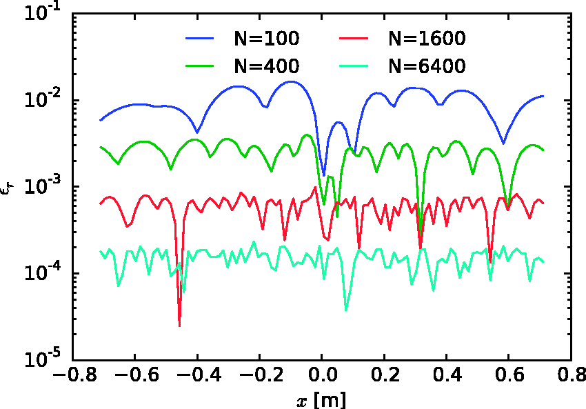$2 π$ .

The microphone time histories for the three monopole case are synthesized based on Gaussian-distributed random source signals. The signals have a duration of 10 s and are sampled at a rate of 51,200 Hz. The propagation from the sources to the microphone positions is calculated using ray tracing. The microphone time histories are then calculated as the sum of all source signals propagated to the respective microphone position. As a basis for the analysis of this data, a cross spectral matrix is computed. The time histories are partitioned into 1000 blocks of 1024 samples each and a Hanning window is applied to each block before an FFT and subsequent power spectrum average with 50% block overlap is performed.

The data for the three monopole case are analyzed using a standard frequency domain beamforming approach with a steering vector formulation of type IV.¹⁶ Figure 8 shows source maps for the 10 kHz third octave band in the x–y plane parallel to the array. If no flow is considered, the map does not show the correct source positions. With the assumption of a thick shear layer, correct positions are found for all three sources. Finally, the assumption of a thin shear layer gives nearly correct source positions with only a slight shift downstream. It can be argued that even in this synthetic case that is set up for a relatively distinct shear layer refraction effect, the consequences of a thin shear layer assumption are not very severe.

Figure 8.

Example application: three point sources in a jet, beamforming source maps for the 10 kHz third octave band (sound pressure level in decibels in the array center) in the plane z = 0.5 m, crosses mark the correct source positions. (a) Computed without shear layer (no flow assumption), (b) computed with thick shear layer, and (c) computed with thin shear layer.

Measurement: Airfoil in open jet

The application of the ray casting approach to a practical measurement is demonstrated here for the case of an airfoil in an open jet aeroacoustic wind tunnel as shown in Figure 1. The tunnel has a nozzle diameter of 0.2 m and an exit velocity of 86.9 m/s ( $M \approx 0.25$ ). The microphone array has 56 microphones with an aperture of 1.3 m and is mounted 0.72 m above the airfoil and the jet center line (similar to the setup in Geyer et al.¹⁷). The airfoil is a NACA 0012 with 0.2 m chord, a span of approximately 0.4 m and was mounted at zero angle of attack with the leading edge 0.05 m downstream from the nozzle. The airfoil span is wider than the jet, so the airfoil protrudes from the shear layer and interacts with it. The inflow turbulence intensity is very low.¹⁸ Consequently, sound generation is expected to happen mainly at the trailing edge. Additionally, the interaction of the shear with leading and trailing edge is also a possible sound source.

The microphone signals were sampled at 51,200 Hz and acquired for 40 s. For the estimation of the cross spectral matrix, the time histories were partitioned into 1000 blocks of 4096 samples each. A Hanning window was applied to each block and an FFT and subsequent power spectrum average with 50% block overlap were used. Again, a beamforming approach with a steering vector formulation of type IV was applied. The mapping grid had a resolution of 0.005 m and 7452 grid points.

Figure 9 shows sound maps for the 12.5 kHz third octave band. If the shear layer refraction is neglected, all expected sources are found, but their location is obviously not correct, but shifted downstream by different distances. Most notably, the trailing edge noise source appears to be shifted in the downstream direction, away from the true location of the trailing edge. If computed using ray casting (N = 800) and a thick shear layer assumption, all sources appear at the expected locations. For the thin shear layer, nearly the same result is computed with a downstream shift of the trailing edge source that is barely noticeable. It can be concluded that the ray casting approach leads to reliable results also when applied to data from a practical measurement. While the assumption of a thick shear layer seems to have only little advantage in the present case, the model is more realistic and the ray casting approach can accommodate more general flow regimes at the same time (e.g. curved shear layers).

Figure 9.

Example application: NACA 0012 airfoil in an open jet aeroacoustic wind tunnel, flow is from left to right, beamforming source maps for the 12.5 kHz third octave band (sound pressure level in decibels in the array center) in the plane z = 0.72 m, blue outline marks the airfoil (chord 0.2 m), dashed lines: shear layers. (a) Computed without shear layer (no flow assumption), (b) computed with thick shear layer, and (c) computed with thin shear layer.

Conclusion

A new method is introduced to handle shear layer refraction in the context of microphone array measurements in open wind tunnel test sections. This method is a ray casting method based on ray tracing. A large number of rays are traced simultaneously and the results are spatially interpolated. This alleviates the need for the application of the iterative procedure of a shooting method necessary for ray tracing between two fixed locations such as source and microphone. While possibly being as accurate as ray tracing, ray casting is much more efficient. The method can handle general cases with no restriction regarding shape and thickness of the shear layer. It is demonstrated using one simulation scenario with three monopole sources within a jet as well as using measurements at a NACA 0012 airfoil in an aeroacoustic wind tunnel.

Footnotes

Acknowledgements

The author is indebted to Kai Liu for performing the measurements on the NACA 0012 airfoil as well as to Mario Wolf and Thomas Geyer for helpful discussions. This paper is based on that presented at the 22nd AIAA/CEAS Aeroacoustics Conference, 30 May–1 June 2016, Lyon, France as AIAA-2016-2762.

Declaration of conflicting interests

The author(s) declared no potential conflicts of interest with respect to the research, authorship, and/or publication of this article.

Funding

The author(s) received no financial support for the research, authorship, and/or publication of this article.

References

Amiet

. Refraction of sound by a shear layer. J Sound Vib 1978; 58: 467–482.

Morfey

Joseph

. Shear layer refraction corrections for off-axis sources in a jet flow. J Sound Vib 2001; 239: 819–848.

Casalino

. Finite element solutions of a wave equation for sound propagation in sheared flows. AIAA J 2012; 50: 37–45.

Padois

Prax

Valeau

. Numerical validation of shear flow corrections for beamforming acoustic source localisation in open wind-tunnels. Appl Acoust 2013; 74: 591–601.

Jiao J, Delfs J and Dierke J. Towards CAA based acoustic wind tunnel corrections for realistic shear layers. In: Twenty-first AIAA/CEAS aeroacoustics conference, no. AIAA 2015-3278, Dallas, Texas, 22–26 June 2015. New York: American Institute of Aeronautics and Astronautics.

Redonnet S and Bulte J. Numerical investigation of the refraction effects by jet flows in anechoic wind tunnels, with application to NASA/LaRC quiet flow facility. In: Twenty-first AIAA/CEAS aeroacoustics conference, no. AIAA 2015-3268, Dallas, Texas, 22–26 June 2015. New York: American Institute of Aeronautics and Astronautics.

Uginčius

. Ray acoustics and Fermat’s principle in a moving inhomogeneous medium. J Acoust Soc Am 1972; 51: 1759–1763.

Candel S. Application of geometrical techniques to aeroacoustic problems. In: Third AIAA aeroacoustics conference, no. AIAA 76-546, Palo Alto, California, 20–23 July 1976. New York: American Institute of Aeronautics and Astronautics.

Candel

. Numerical solution of conservation equations arising in linear wave theory: application to aeroacoustics. J Fluid Mech 1977; 83: 465–493.

10.

Pierce

. Acoustics: an introduction to its principles and applications, New York, NY: American Institute of Physics, 1989.

11.

Dougherty

Beamforming in acoustic testing. In: Mueller

(ed). Aeroacoustic measurements, Berlin Heidelberg, Germany: Springer, 2002, pp. 62–97.

12.

Geyer

Sarradj

Giesler

. Application of a beamforming technique to the measurement of airfoil leading edge noise. Adv Acoust Vib 2012; 2012: 1–16.

13.

Albertson

Dai

Jensen

. Diffusion of submerged jets. Trans Am Soc Civ Eng 1950; 115: 639–664.

14.

Sarradj E. A Python framework for microphone array data processing. Appl Acoust 2017; 88; 50–58.

15.

Brown

Byrne

Hindmarsh

. VODE: a variable-coefficient ODE solver. SIAM J Sci Stat Comput 1989; 10: 1038–1051.

16.

Sarradj

. Three-dimensional acoustic source mapping with different beamforming steering vector formulations. Adv Acoust Vib 2012; 2012: 1–12.

17.

Geyer

Sarradj

Fritzsche

. Measurement of the noise generation at the trailing edge of porous airfoils. Exp Fluids 2010; 48: 291–308.

18.

Sarradj

Fritzsche

Geyer

. Acoustic and aerodynamic design and characterization of a small-scale aeroacoustic wind tunnel. Appl Acoust 2009; 70: 1073–1080.