Flow and noise from septa nozzles

Introduction

This model-scale investigation addresses basic features of flow and noise from a distributed propulsion system.^1,2 In such a system, the exhausts of multiple propulsors are gathered into a common stream at or just before the exit of the nozzle. The concept, considered for some modern aircraft designs, provides for advantages such as in ease of integration of the propulsion system with the airframe. In one version of the concept each propulsor duct is to be driven by an electric fan, the power being generated by engines suitably mounted on the airframe. With such a “hybrid” system the need for heavy power trains is eliminated and system studies indicate numerous benefits at the vehicle level; for a discussion of pros and cons, see Felder et al. ¹ From an aeroacoustics point of view, however, there are concerns and questions. An immediate question is whether the noise from the multiple jets would be equal to or greater than that from an equivalent single jet. When multiple jets are placed side by side sometimes they interact and may produce more noise. In order to address these issues, an experimental study is carried out at NASA Glenn Research Center (GRC).

Preliminary results of the study were presented in a conference paper. ³ One of the key findings was that the noise from the septa nozzle could actually be less than that from the equivalent single nozzle. Continued study made it apparent that the flow as well as the radiated noise could be quite sensitive to the geometry of the passages of the individual propulsion ducts. Specifically, it was shown in Zaman et al. ³ that two septa nozzles of identical design produced very different flowfields apparently due to slight irregularities in the fabrication. Instead of remaining symmetric the cellular flow structure from one nozzle went through a pairing process downstream whereas no such pairing occurred with another; the discrepancy is further discussed in the following. An objective of the continued study was to investigate this anomalous behavior and obtain a clearer understanding of the impact of variations in the geometry of the propulsion ducts on the flow and noise. Key results of the entire investigation were summarized in another conference paper. ⁴ The present paper is a revised version of Zaman et al. ⁴ ; it is contributed for a special edition of IJA celebrating the lifetime achievements of Prof. Dennis K. McLaughlin who, in one way or another, touched and enriched the careers of both authors of the paper.

Experimental facility and procedure

An open jet facility at NASA GRC (referred to as “CW17”) is used for the experiment. Compressed air passes through a 30″ diameter plenum chamber before exhausting through the nozzle into the ambient of the test chamber. Only cold (unheated) flows are considered and further description of the facility can be found in earlier publications.^3,5 A picture of the facility is shown in Figure 1(a). An 8:1 aspect ratio nozzle, referred to as “NA8Z,” ³ is used in the investigation. The exit of the nozzle has dimensions of 5.339″ × 0.658″ and thus an equivalent diameter, D = 2.12″. Figure 1(b) shows the nozzle with a single hot-wire probe in the foreground. Detailed hot-wire surveys at a low Mach number as well as Pitot probe surveys at high Mach numbers are conducted. OPEN IN VIEWER

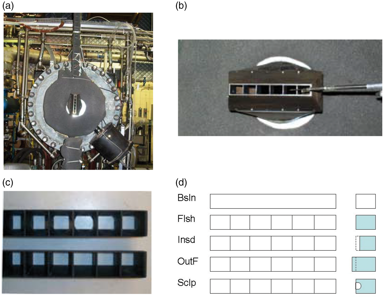
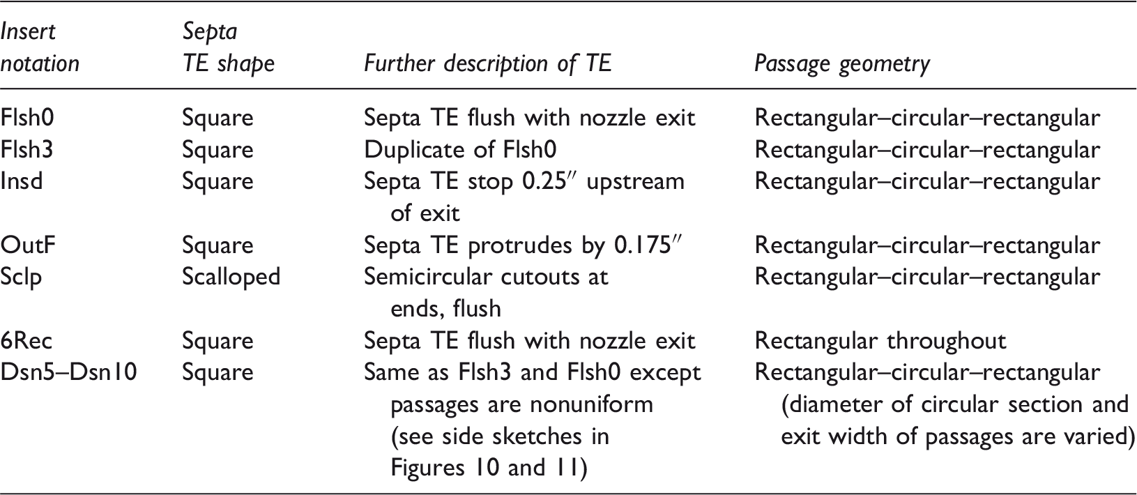
The septa geometry is created by placing an insert into the nozzle. The insert fits snugly and is held in place under flow because of the convergent geometry of the nozzle. All data presented in this paper are obtained with inserts having six passages (or ducts) separated by five septa (or partitions). These were fabricated by additive manufacturing process (3D printing). Figure 1(c) shows pictures of two inserts having different internal passage geometries. The view is from the upstream end. For the one on the top, each passage starts with an almost square entrance, transitions to a circular cross-section and then transitions back to a rectangular exit. The circular cross-section would be the location of the electric fan in the hybrid propulsion system. For the one at the bottom, the passage is rectangular throughout. This represents a simpler geometry with difference in the flowlines within the passages but having identical cross-sections at the entrance and the exit of the passages, as with the other one. These two inserts are referred to as the “Flsh3” and the “6Rec” cases, respectively; the notations are discussed shortly. In both cases the flow continually converges throughout the passage.

As reported in Zaman et al., ³ various other septa geometries (all with rectangular–circular–rectangular passages, as with the Flsh3 case) were tried in an effort to find maximum noise reduction. Four of those are shown by the schematics in Figure 1(d). These will be examined for flowfield and noise details. For these cases, only the trailing edge geometry of the septa separating the passages is varied. The “Flsh” case has the septa ending flush with the nozzle exit. Over time, several 3D prints of the “Flsh” case were used in the experiment; data from two of them, the original one referred to as “Flsh0” and a later one referred to as “Flsh3,” will be discussed in this paper. The “Insd” case has the septa stopping 0.25″ inside from the exit. The “OutF” case has septa protruding out with full width by 0.175″. The septa in the “Sclp” case are scalloped at the end (semicircular cutout). The geometries are depicted in the side views in Figure 1(d). The overall features of all inserts are described in Table 1. Data from all cases are compared with that from the baseline case without any insert (denoted as “Bsln”).

OPEN IN VIEWER

Table 1.

Geometries of septa trailing edge (TE) and passages in various inserts.

Insert notation	Septa TE shape	Further description of TE	Passage geometry
Flsh0	Square	Septa TE flush with nozzle exit	Rectangular–circular–rectangular
Flsh3	Square	Duplicate of Flsh0	Rectangular–circular–rectangular
Insd	Square	Septa TE stop 0.25″ upstream of exit	Rectangular–circular–rectangular
OutF	Square	Septa TE protrudes by 0.175″	Rectangular–circular–rectangular
Sclp	Scalloped	Semicircular cutouts at ends, flush	Rectangular–circular–rectangular
6Rec	Square	Septa TE flush with nozzle exit	Rectangular throughout
Dsn5–Dsn10	Square	Same as Flsh3 and Flsh0 except passages are nonuniform (see side sketches in Figures 10 and 11)	Rectangular–circular–rectangular (diameter of circular section and exit width of passages are varied)

OPEN IN VIEWER

Table 2.

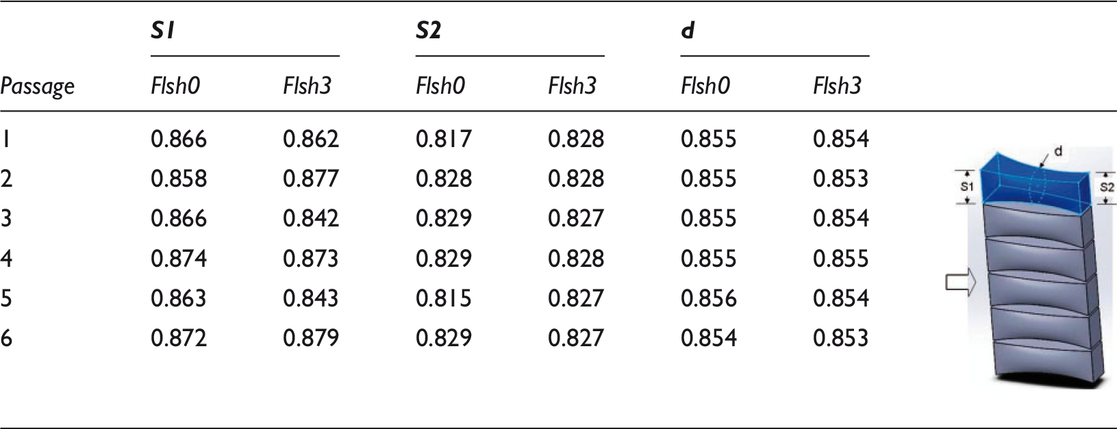
Passage dimensions (inches) for Flsh0 and Flsh3 inserts. The widths S1, S2 and the circle diameter d are defined in the sketch on right.

Passage	S1		S2		d
	Flsh0	Flsh3	Flsh0	Flsh3	Flsh0	Flsh3
1	0.866	0.862	0.817	0.828	0.855	0.854
2	0.858	0.877	0.828	0.828	0.855	0.853
3	0.866	0.842	0.829	0.827	0.855	0.854
4	0.874	0.873	0.829	0.828	0.855	0.855
5	0.863	0.843	0.815	0.827	0.856	0.854
6	0.872	0.879	0.829	0.827	0.854	0.853

The test cell has acoustic linings on the ceiling and upper walls. With proper preparation, qualitative noise measurements are possible. For the present study, comparative spectral levels from geometry to geometry were examined and the facility was considered adequate for that purpose. Microphones (¼″, B&K 4135) held fixed on an overhead arm were used to obtain the noise data. The microphone polar angle (θ) was referenced with respect to the jet’s downstream axis. Spectral analysis was done over 0–50 kHz with a bandwidth of 50 Hz. All spectral data in this paper pertain to a microphone location on the minor axis plane, that is on the broad side of the nozzle. These data are presented as measured and no correction or normalization is applied. Thus, the absolute amplitudes are arbitrary and only the relative change in the amplitude from case to case is considered. Limited noise data were also obtained in GRC’s premium anechoic facility, the Aeroacoustic Propulsion Laboratory (AAPL), ⁶ in order to confirm the trends found in CW17. Presentation format for the latter data are discussed with the results.

A single hot-wire was used for flowfield surveys at low jet Mach numbers (M_j). Limited data at low M_j were also obtained with X-wire probes. A rake of three Pitot probes was used for flowfield surveys at high M_j. Further details of the measurements are discussed along with the relevant results. All dimensions quoted in the paper are in inches.

Flow simulations were made along with the design iterations during the investigation. Reynolds-Averaged Navier–Stokes simulations were made using the Mentor Graphics flow simulation package ⁷ sold by Dassault Systemes with their SolidWorks™ computer-aided design (CAD) software. This industrial-grade flow solver uses immersed boundary meshing and a relatively simple k − ɛ turbulence model to readily produce a credible flow solution using a desktop computer for most subsonic problems. The nozzle flow lines were created in the SolidWorks™ CAD package and the flow simulation results were used in screening the nozzle flow concepts and for confirming the overall flow features observed in the experiment.

Results

Figure 2 compares sound pressure level (SPL) spectra at two jet Mach numbers (M_j = 1 and 0.9). The data are for θ = 90° on the broad side of the jet. Comparison between the flush (Flsh3) and the baseline (Bsln) cases is made in Figure 2(a). For the Flsh3 insert, there is a significant reduction of the spectral amplitudes at low frequencies. With the insert there is flow blockage; the equivalent diameter is smaller by about 12%. It is estimated that the reduction in spectral amplitudes due to the blockage should be about 1.13 dB. The amplitudes on the low frequency end have reduced in excess of 5 dB and thus cannot be due only to area blockage. SPL spectra for the case with rectangular passages throughout (6Rec) are shown in Figure 2(b). Here, the comparison is made between the 6Rec case and the Flsh3 case (the two inserts of Figure 1(c)). Clearly, the case with rectangular–circular–rectangular passage (Flsh3) yielded more noise reduction. A comparison with the data in Figure 2(a) makes it clear that the 6Rec insert also reduced noise relative to the Bsln case but not as much as obtained with the Flsh3 insert. OPEN IN VIEWER

Similar comparisons of the SPL spectra for the other cases of Figure 1(d) are shown in Figure 3(a) to (d). Again, in each figure the data for an individual case are compared with Flsh3 data. It is apparent that with both the Insd and the OutF cases (Figure 3(a) and (b)) the noise reduction is not as much as with the Flsh3 case. The Sclp case in Figure 3(c) is seen to be as effective as the Flsh3 case. Many other designs were tried in Zaman et al. ³ and the Flsh3 (or Flsh0) design produced the most noise reduction. Recall that Flsh3 and Flsh0 cases are 3D prints of the same design. As it will be shown shortly, the two produced quite different flowfields downstream. However, in spite of the flowfield differences the noise results were comparable (Figure 3(d)). Close scrutiny suggests that the Flsh0 case may have yielded slightly better noise reduction. OPEN IN VIEWER

A brief experiment was conducted in GRC’s anechoic facility AAPL (“Experimental facility and procedure” section). The same NA8Z nozzle with and without the Flsh0 insert was used. Spectral data, from 24 polar locations (microphones on the minor axis plane, ϕ = 0°), are shown in Figure 4(a) for M_j = 0.99. The data (power spectral density referenced to 1 ft distance) are shown as a “carpet plot.” Note that the amplitude difference between the Bsln and the Flsh0 cases (“dPSD” in dB) is also superimposed in this plot with the color code indicated in the legend. Large decrease in the amplitudes (green-blue region on the right) is noted on the low frequency end. The trend persists at all polar (θ) locations. A direct comparison of the spectral profiles between the Bsln and the Flsh0 cases is made with the line plots in Figure 4(b). For comparison, corresponding pair of spectral traces from CW17 experiment are shown in Figure 4(c). Note that the amplitudes for the latter data are in arbitrary scale and also the frequency range covered is lower. Nevertheless, quite similar differences are observed. Thus, the noise suppression by the septa (Flsh0) case first observed qualitatively in CW17 is confirmed by the accurate AAPL data. OPEN IN VIEWER

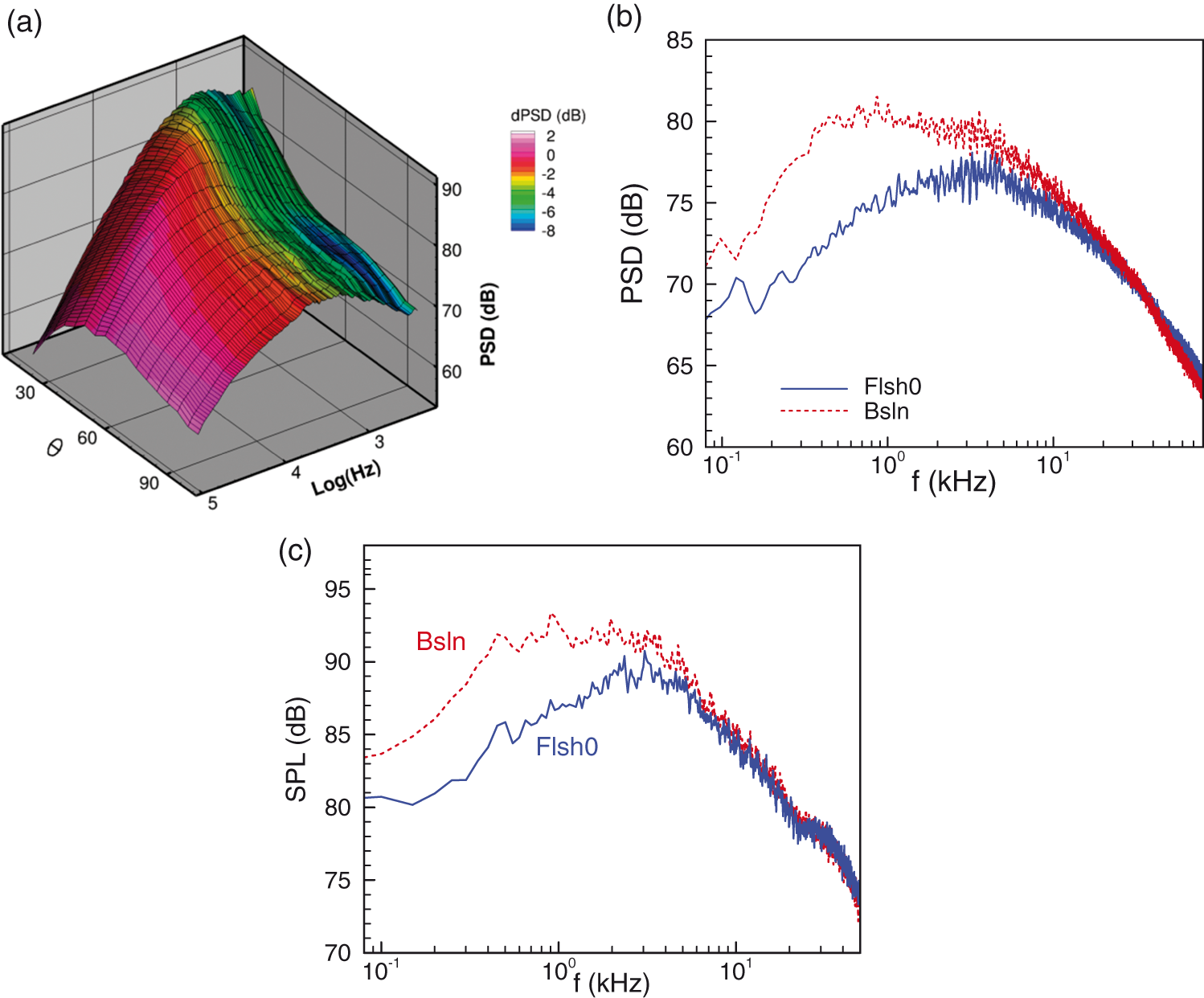
Here, it should be noted that the noise benefit for a full-scale model on a perceived noise level metric may not be as attractive since the noise reduction with the model-scale case is seen mostly on the low frequency end. Furthermore, additional boundary layers with the septa geometry would incur some thrust loss relative to an equivalent single jet. The extent of such losses as well as losses involved in generating the streamwise vortices remains unknown at this time. Based on past experience with chevrons, ⁸ however, the thrust losses might be expected to be tolerable. These issues need to be addressed further before the technique could be embraced at an application level.

The flowfield characteristics for the septa nozzles are explored next. Figure 5 shows hot-wire survey data at x/D = 2; D is the equivalent diameter of the baseline nozzle, as stated in “Experimental facility and procedure” section. Contours of mean velocity (normalized by jet velocity at the nozzle exit) on the cross-sectional plane are plotted for a jet Mach number of M_j = 0.265. The data are for different septa designs as indicated in the caption of Figure 5. For all cases the flow starts as six high-velocity cells just downstream of the nozzle exit (see further data in the following). For the Flsh3 case in Figure 5(a), the six cells have transformed into five high-velocity regions by x/D = 2. This behavior is understandable. There are five septa for the six passages and apparently pairs of streamwise vortices form at the ends of each septum (the septa locations are shown by the dashed lines in Figure 5(a)). The vortex pairs pull the flow outward causing high-velocity flow from adjacent cells to congregate in front of each septum or partition, causing the formation of the five high-velocity regions. OPEN IN VIEWER

Figure 5(b) shows the corresponding velocity distribution for the Flsh0 case. As stated before, this insert was of the same design as the Flsh3 case. However, the flowfield is quite different from that seen in Figure 5(a). By the measurement station at x/D = 2 the six original high-velocity cells have gone through a pairing process to yield three cells. An asymmetry has also developed. Note that the middle cell is not centered at z = 0. The Flsh0 case was the first septa insert tried in this investigation; since then several more inserts of the same design were printed and most showed a behavior as seen in Figure 5(a). The peculiar behavior with the Flsh0 case is due to small differences in the internal geometries of the septa passages. The 3D printing process was not precise; the tolerance was approximately ±0.010″. Small differences in the dimensions from septum to septum were possible even though nothing was visually obvious. The flowfield difference between Figure 5(a) and (b) is the anomalous behavior noted in “Introduction” section. This is pursued further in the following.

Figure 5(c) shows flowfield data for the 6Rec case, at x/D = 2 and M_j = 0.265. There is no pairing activity. Neither is there a transition to five high-velocity regions as seen in Figure 5(a). The six high-velocity cells are still discernible at the measurement station. Recall that this case has rectangular cross-section throughout each passage, as opposed to the rectangular–circular–rectangular geometry with the Flsh3 case. The difference in the internal passage geometry made a significant difference in the flowfield as well as in noise (Figure 2(b)). The three other cases in Figure 5 with various shapes of the septa ends, all with rectangular–circular–rectangular internal passage, exhibit similar patterns as seen for the Flsh3 case in Figure 5(a). The high-velocity regions are somewhat diffused for the Insd and OutF cases (Figure 5(d) and (e)). The noise reductions with the latter two cases were not as much as with the Flsh3 case (Figure 3(a) and (b)). Note that the Sclp case (Figure 5(f)) produced almost identical pattern as with the Flsh3 case, and these two also had practically identical noise signatures (Figure 3(c)).

Corresponding flowfield data at a high Mach number (M_j = 0.90) for selected cases are shown in Figure 6. These data at x/D = 2 were obtained by Pitot probe surveys. The patterns for the Flsh3, Flsh0, and 6Rec cases in Figure 6(a) to (c) are quite similar to the patterns seen at low speeds in Figure 5(a) to (c), respectively. These flowfields are a result of streamwise vortex interactions, and obviously those interactions are not affected significantly by compressibility effects. OPEN IN VIEWER

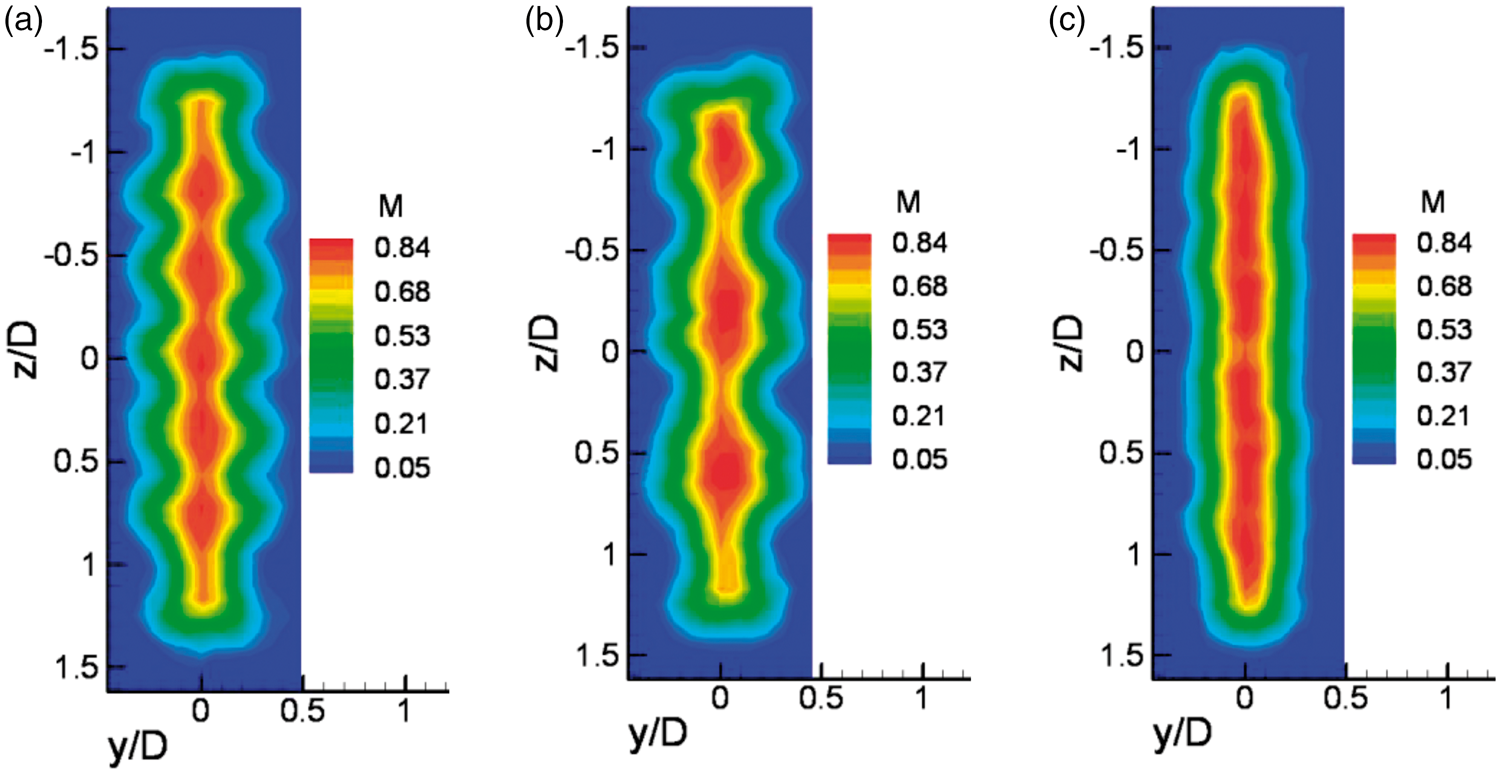
Figures 7 to 9 document the streamwise evolution of the flow for the Flsh3, Flsh0, and 6Rec cases, respectively. These hot-wire data at M_j = 0.265 are shown for five streamwise locations, as indicated. In both Figures 7 and 8, the migration of the flow to form high-velocity regions downstream of each septum can be noted. However, for the Flsh0 case (Figure 8) there is further interaction with increasing downstream distance. Counting from the top, high-velocity regions 1 and 2, and 3 and 4 merge, while region 5 at the bottom is left alone. This is how the asymmetry in the flow develops. In contrast, the five regions for the Flsh3 case (Figure 7) continue to retain their identity until getting diffused by x/D = 4. For the 6Rec case in Figure 9, on the other hand, there is neither an intercell migration nor a pairing activity farther downstream. The six high-velocity cells retain their identity until getting diffused by x/D = 4. It is apparent that streamwise vortex pairs are formed at the ends of the septa for the rectangular–circular–rectangular passage geometry (Flsh3 and Flsh0); limited X-wire data for the Flsh3 case are presented shortly. Such vortices must be absent (or are of minimal strength) in the 6Rec case with the rectangular passage. It is also apparent that some sort of nonuniformity is introduced in the vortices with the Flsh0 case that lead to the subsequent pairing activity. OPEN IN VIEWER

OPEN IN VIEWER

Figure 8.

Evolution of mean velocity field for Flsh0 case. Data shown similarly as in Figure 7. (a) x/D = 0.04, (b) x/D = 0.5, (c) x/D = 1, (d) x/D = 2, and (e) x/D = 4.

OPEN IN VIEWER

Figure 9.

Evolution of mean velocity field for 6Rec case. Data shown similarly as in Figure 7. (a) x/D = 0.04, (b) x/D = 0.5, (c) x/D = 1, (d) x/D = 2, and (e) x/D = 4.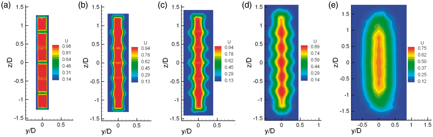

As already stated, the Flsh0 and the Flsh3 cases were fabricated from the same CAD files and were supposed to be identical. Obviously small variations in the septa geometry due to the uncertainty in the fabrication process resulted in the observed difference in the flow. The variations could not be discerned visually or through cursory measurements with calipers. The two specimens were then inspected by optical methods (by Inspection Engineering, Westlake, OH, using an apparatus called “Flash Smartscope”). Dimensions deemed critical are listed in Table 2. The sketch on the side of the table provides definitions of the parameters; S1 and S2 are the widths of a passage at the inlet and outlet, respectively, and d is the diameter of the circular cross-section in the middle. It can be seen that up to 0.024″ differences in the dimensions occurred in certain parameters between the two inserts (see the values of width S1 for passage #3). Thus, the maximum difference was about 2.8% of the design width, and no other gross anomalies in the dimensions stood out. The measurements pertained to the central plane of each passage, and there were variations in the transverse direction. However, from visual inspection variations worse than the observed maximum were unlikely. In any case, these data were not helpful in pinpointing the cause for the difference in the flowfield. At this point, several new inserts were fabricated by deliberately varying the dimensions of the passages. Specifically, the dimensions S2 and d were varied from passage to passage in a systematic manner. The notion was that such variations would change the contraction ratio from the circular to the rectangular exit and thereby affect the strength of the secondary flow that in turn would affect the strength of the streamwise vortices. Flowfield surveys for four such design cases are shown in Figure 10. For each case, data at x/D = 2 and 4 are shown with the design change indicated by the sketch on the left. The changes are as follows. The blue circles indicate that the diameter d was decreased by 0.025″ from the nominal value of 0.855″ while the red circles indicate an increase in d by 0.025″. Similarly, the blue rectangles indicate a decrease in the outlet width S2 by 0.025″ and the red rectangles an increase in S2 by 0.025″. Noting that the 3D printing process is not precise (tolerance approximately ±0.01″) the exact dimension changes are not guaranteed. However, the changes were large enough to affect the overall contraction ratios in the desired directions. OPEN IN VIEWER

From Figure 10 it is apparent that any of the deviations from the standard design may affect the flowfield evolution in some manner. This is evident from the nonuniformity in the spacing of the high-speed regions at x/D = 2, although the effect was only slight and nowhere near as strong as seen with the Flsh0 case. Many other combinations were tried. The closest resemblance with the Flsh0 case was achieved by the design (Dsn9) in Figure 11. Here, both d and S2 were varied to accentuate the effect. A tendency for pairing as with the Flsh0 case can be seen by x/D = 2. By x/D = 4 the flow pattern became quite similar to that seen with the Flsh0 case (Figure 8). OPEN IN VIEWER

Limited Reynolds-Averaged Navier–Stokes flow simulations were conducted during the exploration of geometric impacts. Streamwise evolution of mean velocity data for the Dsn9 case is shown in Figure 12. A similar flowfield evolution is noted as in Figure 11. Corresponding CFD results for the Flsh3 case are shown in Figure 13. When compared with the data in Figure 7, again a very similar evolution can be seen. These CFD results confirm that indeed a small variation in the internal passage dimensions can impact the flowfield quite significantly leading to the flow patterns observed in the experiment. OPEN IN VIEWER

OPEN IN VIEWER

Figure 13.

CFD solution for mean velocity (Mach number) field for Flsh3 case; data shown for five streamwise (x/D) locations as indicated, M_j = 0.27 (compare with Figure 7). (a) x/D = 0.04, (b) x/D = 0.5, (c) x/D = 1, (d) x/D = 2, and (e) x/D = 4.

Finally, X-wire hot-wire measurements were performed for the Flsh3 case in order to explore further details of the flowfield. Two X-wires, one in u–v and another in u–w configuration, were traversed in z through the same grid points and the measurements repeated at various y locations. The two probes were separated by 0.96″ (in z) and the two sets of data were shifted during postprocessing to coincide with each other, providing time-averaged values for all three components of mean velocity and normal stresses at each point. In addition, the Reynolds stresses uv and uw were also obtained. Unfortunately, the spatial resolution of the probes was not good for resolving the fine details of the flow that contained a multitude of vortices. The measurements were carried out only at x/D = 2 in an effort especially to identify the streamwise vortices. Note that the X-wire probes had to be inserted straight into the flow with probe support parallel to the x-direction (the single hot-wire was inserted at an angle and traversed in y-direction in order to minimize probe interference). Thus, only a little over half of the flowfield was covered in the X-wire measurements since interference from the probe support would be large when reaching the far end in negative z. A few of the flow properties are shown in Figure 14. The mean velocity U can be seen to be comparable to the single hot-wire data in Figures 5(a) and 7. For normal stresses, only u′ and v′ are shown while w′ was noted to be very similar to v′ in amplitude and distribution. Peak u′ amplitude (0.163) is found to be much larger than peak v′ amplitude (0.106) or peak w′ amplitude (0.102). The two Reynolds stress data are also shown. Finally, the streamwise vorticity (ω_x) data are shown at the bottom right corner of Figure 14. Even though not orderly and crisp, the ω_x data leave no doubt that pairs of counter rotating vortices occur on either side of the flowfield. The locations of the septa are indicated by the dashed lines. An inspection indicates that indeed vortex pairs of opposite sense occur at the ends of each septum. OPEN IN VIEWER

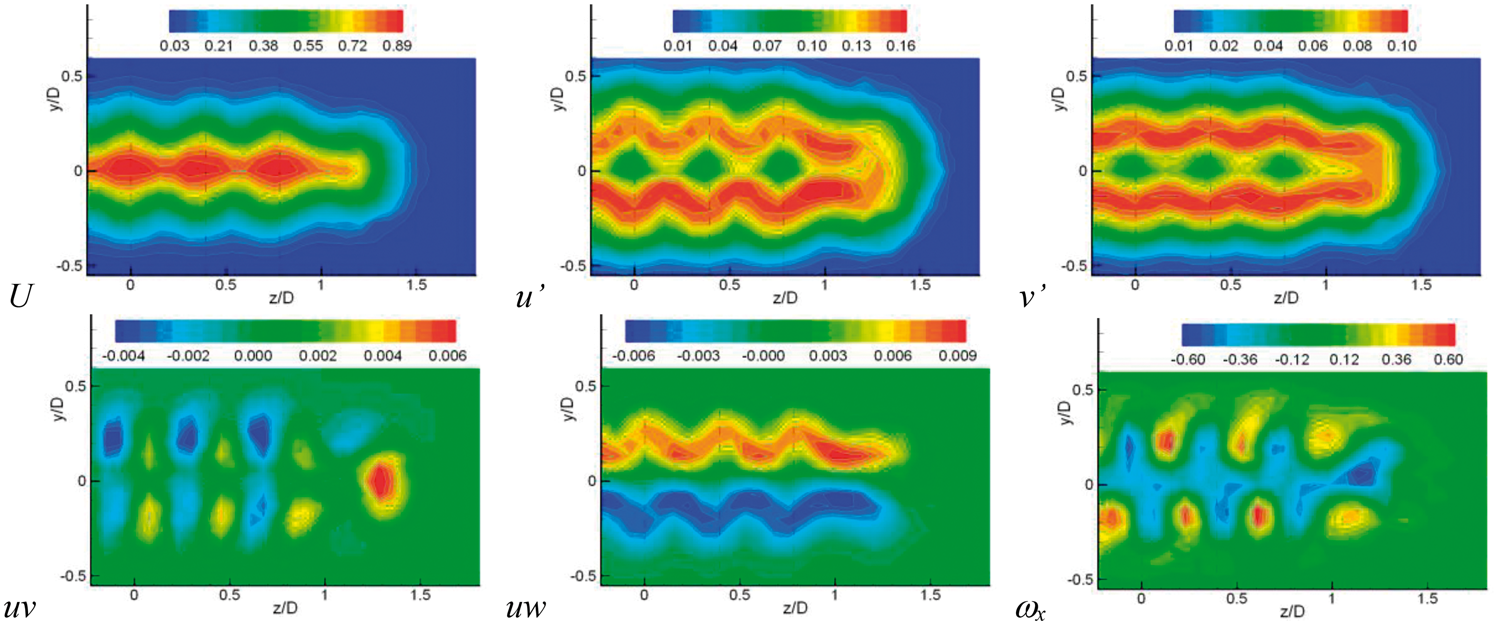
Concluding remarks

A model-scale experiment is conducted with an 8:1 aspect ratio rectangular nozzle that is divided into six passages by five septa. Plastic inserts placed inside the nozzle create the septa geometry. The inserts are fabricated by additive manufacturing process (3D printing). It is found that the noise radiation from the septa geometry can be significantly lower than that from the baseline (no septa) rectangular jet. Up to 5 dB noise reduction is noted on the low frequency end of the spectrum. The septa inserts cause a flow blockage amounting to about 12% reduction in the equivalent diameter of the nozzle. Rough estimates show that this should correspond to about 1.13 dB reduction in noise; thus, the observed noise reduction is not due only to flow blockage.

The noise reduction is found to occur with a septa design where the flow passage goes through a rectangular–circular–rectangular transition. It is noted that when the passage is rectangular throughout there is also some noise reduction that could be mostly due to the flow blockage. Flowfield surveys suggest that pairs of streamwise vortices are introduced with the rectangular–circular–rectangular passages. These pairs occur at ends of each of the five septa that separate the six passages. The vortex pairs pull the flow outward and as a result the six high-velocity cells originally issuing from the nozzle transform into five high-velocity regions shortly downstream. In contrast, with the rectangular-throughout passage case the six cells retain their identity far from the nozzle exit until getting diffused due to turbulence. This suggests that there are no significant streamwise vortices in the latter case. From these considerations it may be inferred that the introduction of the streamwise vortices in the former case is at the root of the noise reduction.

The introduction of the streamwise vortices and the resultant evolution of the flowfield are found to be sensitive to upstream passage geometry. In fact, much of the effort in the investigation was prompted by an “anomalous” behavior noted earlier in the study. Two septa inserts fabricated with the exact same design produced very different flowfields. In one, the six high-velocity cells produced five regions of high-velocity flow, as discussed in the previous paragraph. In another, the five regions went through a further pairing process that produced an asymmetric flowfield with three high-velocity regions. It is inferred that this difference in behavior resulted from slight imperfections in the geometries of the latter insert due to inherent inaccuracies in the 3D printing process. This was pursued by deliberately introducing nonuniformities in the dimensions of adjacent septa. Eventually with certain changes in the dimensions a similar “anomalous” flowfield could be reproduced. Limited numerical simulation with the latter design confirmed the observed development of the flowfield.

While most of the flow data presented in the paper pertain to a low jet Mach number it was found that the flow pattern observed with a given insert was the same at a high subsonic Mach number. Thus, the distribution and interaction of the streamwise vortices affecting the flow evolution must be largely independent of compressibility effects.

Therefore, the rectangular–circular–rectangular passage within a flow duct, necessary in electric propulsion (the fan has to be located at a circular cross section), has an added benefit of producing some noise reduction. The noise reduction stems from the introduction of streamwise vortices, which are apparently produced by secondary flow in the transitional passages. The key lesson of this work is that the strength and distribution of those vortices can be sensitive to the exact geometry of the passages. This should be borne in mind in the design of a distributed propulsion system and in fact may be taken advantage of for tailoring the flowfield downstream as well as for achieving some noise reduction.