Jet mixing noise is experimentally investigated by means of cross-correlations between density fluctuations inside the turbulent jet flow and the far-field acoustic pressure. The time-resolved density fluctuations are measured by an experimental device based on Rayleigh scattering, which is mounted in the large anechoic wind tunnel of Ecole Centrale de Lyon. An original signal processing developed in a previous study is implemented for the photon counting, combined with the use of a single photomultiplier to remove shot noise. A high-speed subsonic jet and a perfectly expanded supersonic jet with a subsonic convective velocity are considered to characterize mixing noise sources. In order to go beyond the classical Fourier analyses, conditional cross-correlations are determined, and the signature of turbulent events linked to the noise emission in the downstream direction is extracted.
The noise of subsonic turbulent jets remains a stimulating research topic in aeroacoustics. In particular, many clever analyses have been carried out with the aim of connecting turbulent events inside the flow with the sound emission in the far-field. With that in mind, however, a direct approach based on Fourier analysis through cross-spectra and correlations is often disappointing. It has been shown on the contrary that the use of conditional means associated with the intermittent feature of jet turbulence and noise can provide insightful information.1–6 Noise generation mechanisms related to turbulent events leading to dominant acoustic emission can be detected by computing a conditional cross-correlation between the turbulent velocity field, and more precisely vortical structures, with the far-field sound pressure fluctuations. Many findings have resulted from these experimental measurements and more recently from numerical studies. Examples of such results include the presence of a noise generation mechanism at the end of the potential core, linked to the periodic and intermittent intrusion of accelerated vortical structures into the jet core. In this context, a notable exception in the way in which correlations are defined is the experimental work performed by Panda et al.7 Cross-correlations are formed from the density fluctuations inside the turbulent flow region and the radiated acoustic pressure field. This has been made possible with the use of a Rayleigh scattering-based technique to measure time-resolved density fluctuations in a non-intrusive manner.
In addition to the characterisation of aeroacoustic sources through the identification of direct links between the turbulent flow and the emitted sound, previous work involving time-resolved schlieren visualisations to study supersonic jet noise8,9 has stressed the interest of having a direct absolute measurement of the density. Furthermore, there is also a lack of well-documented experimental data for compressible turbulent jets. A direct measurement of the density fluctuations and the possibility of determining density spectrum or correlations between density and velocity are therefore attractive challenges.
The paper is organized as follows. The principle of the Rayleigh scattering is briefly introduced in the next section. The experimental setup and the specific signal processing required for the photon counting10 and for two-point statistics are then described. The following sections are devoted to the presentation of the experimental results, and in particular to the extraction of the conditional average of the density fluctuations linked to the acoustic emission in the downstream direction of a subsonic jet at Mach and a perfectly expanded jet at . Concluding remarks are finally drawn in the last section.
Density measurement by a Rayleigh scattering-based method
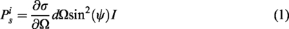
Rayleigh scattering corresponds to the elastic scattering of light by particles small in comparison with respect to the incident light wavelength.11 Considering that the incident light is polarized and interacts with a particle of differential scattering cross-section (), the power in W of the scattered light collected into a solid angle (sr–1) in a direction that forms an angle ψ with the electric vector is given by
where I is the irradiance in of the incident light. In the present study, the particles of interest are the molecules that constitute the gas flow. The numeric density (m–3) of molecules in air is related to the density ρ (), the molecular mass () and the Avogadro constant NA () by
The total collected power Ps is the sum of all particle contributions. For a probe volume Vsc (m3) that contains molecules, the scattered power Ps can thus be recast as
An estimate of the power of scattered light based on the numerical values provided in Table 1 for the present experimental setup leads to W. The measurement of such a small amount of power will turn out to be difficult, but this quantity is nevertheless of interest for flow diagnosis in fluid dynamics, in particular for density measurement. An indirect determination of Ps is achieved by photon counting in practice. The scattered collected light power can be converted into a photon flux (photons per second), which yields
where h () is the Planck constant, c () is the speed of light and λ (m) is the wavelength. The flux of photons is obtained by counting photon arrival rate in the practical setup. A photomultiplier is used to convert photon detections into electric pulses that are digitized by an acquisition unit with a high sampling rate. Such a sensor is characterized by an intrinsic quantum efficiency QE, which is the probably to detect a photon that reaches the sensor. Typically, between 10 and 50% of the collected photons are detected. The detected flux of photons is finally given by
Typical values of the Rayleigh scattering bench for .
λ
532
nm
Vsc
m3
I
kg–1
ψ
rad
sr
QE
0.3
Ps
W
photons per second
For a given light wavelength and intensity and a given gas flow, the scattered collected light power Ps is found proportional to the density
The coefficient k is setup-dependent in equation (6) and can be determined from a specific calibration process, as detailed in Panda and Gomez.12
Experimental setup
The present experiments are conducted in the anechoic wind tunnel of the Centre for Acoustic at École Centrale de Lyon. A sketch is shown in Figure 1. This wind tunnel is equipped with a high-pressure compressor to produce a continuous pressurized air flow. The air is blown in a duct at the end of which a nozzle is located.9 Two different nozzle geometries are considered in this study, a D = 38 mm diameter convergent nozzle and a convergent-divergent nozzle of throat diameter 38 mm and of exit diameter mm. The notation Dj = D for the convergent nozzle and Dj = De for the convergent-divergent nozzle will be used throughout the text to define the Reynolds number , for instance, where ρj is the nominal jet density, is the dynamic viscosity and Tj is the static temperature. The operating conditions of the wind tunnel are set so that a jet develops downstream of the convergent nozzle. The total temperature of the subsonic jet is approximately 30°C and the Reynolds number . A supersonic jet is also considered with a ideally expanded jet obtained downstream of the convergent-divergent nozzle. The Mach 1.32 jet is slightly heated up to a total temperature of 70°C. This results in a jet temperature of –19° that prevents the condensation of water droplets downstream of the nozzle exit, and the Reynolds number is . Air filters are arranged at the compressor inlet and downstream of the heater, in order to clean the flow from dust particles. A secondary nozzle, coaxial to the primary one and with a diameter of 200 mm, is also supplied with filtered air. The velocity of this co-flow is 10 m/s, and this secondary stream is only used to feed the entrainment induced by the primary jet with clean air. Rayleigh scattering-based methods indeed require the least amount of dust particles in the flow. The co-flow also defines the ambient temperature that varies here between 16 and 19°C.
Sketch of the wind tunnel and Rayleigh scattering apparatus.
The radiated acoustic field is recorded from a 13-microphone polar antenna of radius 50D centred at the nozzle exit. The microphones are set from to every 10°, the angle θ being measured with respect to the jet axis in the downstream direction.
The light source used for the present Rayleigh scattering measurements is a 532 nm continuous 5 W laser beam with a diameter of 1 mm. The scattered light is collected by a lens of focal length f = 450 mm and aperture . The light is then focused by a second lens on a slit and is finally focused on a photomultiplier. The size of the slit defines the size of the probe volume. Here, the probe volume is a cylinder of diameter equal to the laser beam diameter and of 0.3 mm in height. The photomultiplier is a Hamamatsu H7422-P40, connected to a data acquisition card NI-5160 with a maximum sampling rate of 2.5 GHz. Such a high value is required to digitize the pulses from the photomultiplier output signal, which are directly associated with the photon detection. The recording time is limited by the card memory to 0.86 s when the sampling rate is chosen to be 1.25 GHz. More details about the data acquisition are provided in a previous reference10 and are not reproduced here. The laser and the light collectors are supported by a rigid fame mounted on a two-axis traverse system. In order to reduce possible acoustic reflections on the frame, the latter has partly been coated with acoustic foam.
Signal processing
Photon counting
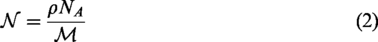
The signal recorded by the data acquisition card is the output signal of the photomultiplier. A sample record is shown in Figure 2. The signal consists of discrete spikes of random amplitude and of a low-level electronic noise. It is first necessary to detect the photon signature in the signal in order to obtain a time series representative of the time evolution of the photon flux, and hence the density according to equation (6). This is done by seeking the peaks that are above a given threshold. The time arrival of all detected photons is then gathered. For a given sampling frequency fs of the density time series, successive time bins of length are introduced. The sampling frequency is here chosen to be the same as the acoustic acquisition, that is fs = 204,800 Hz. The photon arrivals are finally sorted in their corresponding time bin as a function of their arrival time. The number of photons N(t) per time bin is finally converted into the counted photon flux by
Sample of a photomultiplier output signal digitized at a sampling rate frequency of 1.25 GHz; photon arrivals, threshold.
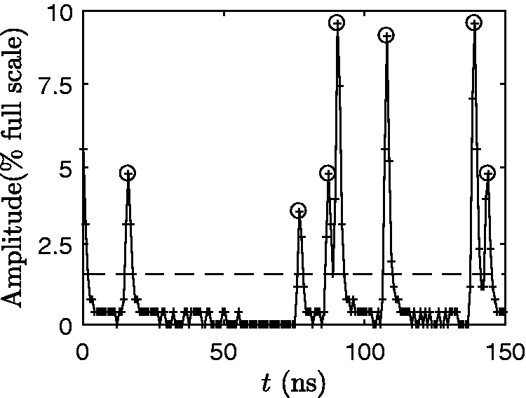
It should be noted that is not strictly equal to , and thus proportional to the density. Indeed, if the pulses associated with two consecutive detections are superimposed, only one of the two can be counted. The minimum delay for two detections to be properly counted is the pulse pair resolution τ. For the present experimental device, τ is approximately equal to 1.5 ns. As a consequence, the flux of counted photons is underestimated, but the correct value in equation (6) can be recovered from the following expression10
obtained by modelling the pileup effect.
A last consideration about photon counting must be pointed out. Photon arrivals are randomly distributed and follow a Poisson distribution. Therefore, even for a constant scattered light power, the number of detected photons N during two independent time bins might be different. These variations produce a random noise that adds to the expected value and is called shot noise. From the properties of Poisson’s distribution, the standard deviation of the shot noise σSN is given by
The time series measured by photon counting is therefore proportional to the scattered power, and so the density, but only in average. If the calibration coefficient is applied to the instantaneous in equation (6), the result will be related to the density, but with a relative error varying as .
Density – pressure coherence
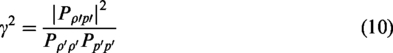
The time series representing the density obtained from photon counting were simultaneously acquired with the far-field acoustic pressure . The spectral coherence is the first quantity considered for investigating noise emission. The coherence is defined as
where the density and pressure spectra are denoted as and , respectively, while the cross-spectrum between and is . In order to account for the causality between the source and the observer, the acoustic signal is time shifted by the acoustic propagation delay.5 The propagation delay is estimated by assuming a free-field propagation in an ambient medium at rest between the probed location by Rayleigh diffusion inside the jet flow and a given microphone.
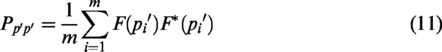
In order to evaluate and , the density and pressure signals are divided into m segments of length close to 4 ms to obtain a frequency resolution of 0.025 St, where the Strouhal number is defined as St = . The segments are noted and , with 50% overlap, and with for . The power spectral density of the pressure is given by
and the cross-spectrum by
where the operator denotes the Fourier transform and * is the complex conjugate. Since the shot noise contained in density signals is not correlated with the pressure, the cross-spectrum is independent of the shot noise level. This is true as long as m is large enough, which applies in the results presented in this study.
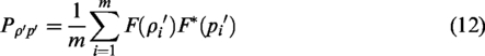
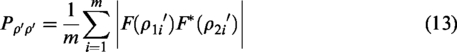
On the contrary, a specific treatment has to be applied for determining . At least two strategies may be implemented to overcome the influence of this undesirable component. A first method13 consists in measuring the density at the same point simultaneously with two distinct sensors. The density fluctuations measured by the two sensors are the same but the shot noise contributions are not correlated and do not contaminate the cross-spectrum. A second approach has been recently developed and validated by the authors,10 using a single photomultiplier. The primary signal of sampled every dt is divided into two signals and , coherent in terms of density fluctuations but independent in terms of shot noise. The first signal is made from the samples of at while the second is made from the samples at , for . If dt is small in comparison with the turbulence time scale, thus if the sampling frequency is chosen high enough, the contribution of density fluctuations in the two signals is identical, but shifted by dt. These two signals and are finally divided into m segments to estimate the density spectrum
The modulus is necessary to handle the phase shift introduced between ρ1 and ρ2.
Density – pressure cross-correlation
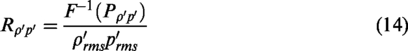
For correlation calculation, the pressure signals are first shifted in time by the propagation delay between the probed volume and the microphone, as for the coherence calculation (equation 10). Panda and Seasholtz13 recommend using the inverse Fourier transform of the cross-spectrum to compute the cross-correlation function instead of using the convolution definition. Both methods have been tested, and better results have actually been obtained using the cross-spectrum. The cross-correlation function is classically normalized by the product of the standard deviations of the density and pressure, which yields
The computation of is carried out from the Parseval identity, by integration of the density spectrum obtained with the method described in the previous section.
In order to reduce the noise in the correlation , all the signals are filtered by a low-pass fourth-order filter of cut-off Strouhal number . It should be noted, however, that calculating requires the successive samples to be independent in terms of shot noise. This condition would not be met if the filter was applied to . The filter is therefore applied to and .
Results
A subsonic jet at and an ideally expanded supersonic jet at are investigated in this work. The aim of this introduction is to provide an overview of the acoustic field and the aerodynamic density fluctuations for these two jets.
Far-field acoustic spectra measured at angles of 30 and 90° are presented in Figure 3 for the and jets. The spectra at are found in good agreement, which confirms the absence of broadband shock-associated noise for the supersonic jet, which is actually ideally expanded. They also compare well with the empirical spectrum determined by Tam et al.14 for fine-scale turbulence. The acoustic spectrum recorded at for the jet is found slightly broader than that found for the supersonic jet, and that derived by Tam et al.14
Sound Pressure Level (SPL) spectra in dB/Hz at and from the flow direction. – , – , – Tam et al.14
Most of the following analyses rely on the correlations between the acoustic pressure measured at , and the density fluctuations measured near the end of the potential core. In this region, the correlation levels are expected to be large enough to be measured.5,13 The length zc of the potential core is estimated from the expression15
that provides and for the two jets. Consequently, the probed points for density measurements are chosen between and . The latter corresponds to the maximum distance achievable before dusty surrounding air in the anechoic room is entrained by the jet. Rayleigh scattering-based measurements are then corrupted.
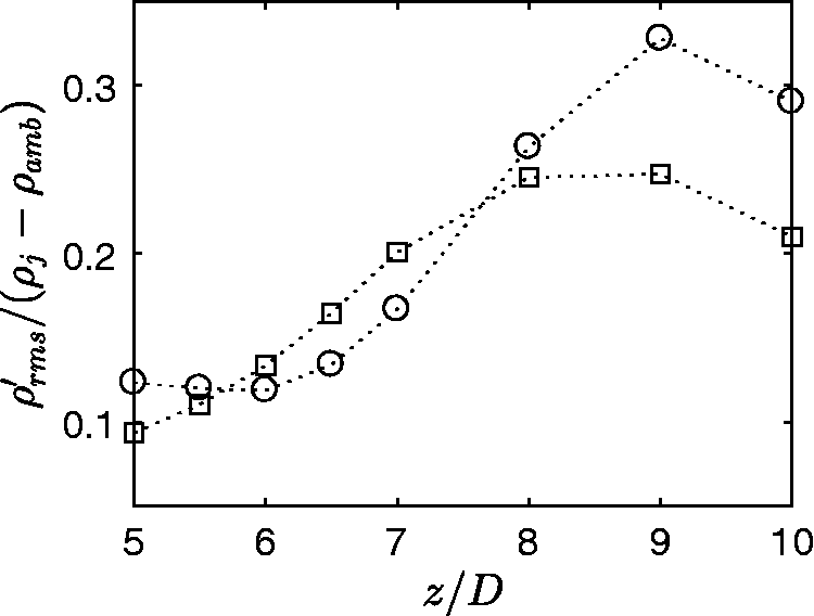
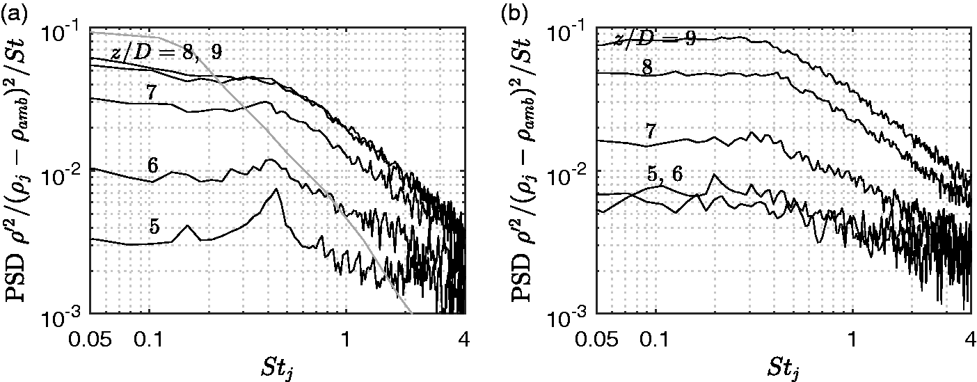
The axial profile of density fluctuations on the jet axis is shown in Figure 4. This profile covers the end of the potential core for both jets. The peak of density fluctuations lies between and for the jet and is close to for the jet. These positions agree well with Panda and Seasholtz measurements13 on similar jets. Density spectra measured along this line are presented in Figure 5. For each axial location, the spectrum is found to be flat below and follows a straight decay at higher frequencies in logarithm scales. The slope seems to increase with the axial position, before reaching a constant value probably associated with a fully developed turbulent state. A bump can be observed at for the spectrum located at the end of the potential core of the subsonic jet. A similar bump at the same frequency is also found at other probed points inside the potential core, these spectra are not shown here to save space. This behaviour has already been observed in the past, see for instance, Figure 3 in Fuchs,16 and a recent interpretation in terms of trapped acoustic waves can be found in Towne et al.17
Axial profile of normalized density fluctuations on the centreline. □ ( kg/m3), ( kg/m3).
Power Spectral Density (PSD) of the density fluctuations at the indicated axial position along the jet axis for (a) and (b) – Velocity spectrum at the end of the potential core for a jet.18
For comparison purposes, a spectrum of velocity fluctuations is also superimposed in Figure 5. It was measured by Kerhervé et al.18 using laser Doppler velocity on the centreline of a jet at the end of the potential core. The shape differs from the density spectrum, with a roll off in frequency from Stj between 0.1 and 0.2, instead of 0.4 for the density spectrum. Furthermore, a spectral slope of −5/3 predicted by Kolmogorov’s theory is found, which is a larger value than for the density spectrum.
Density – far-field sound coherence
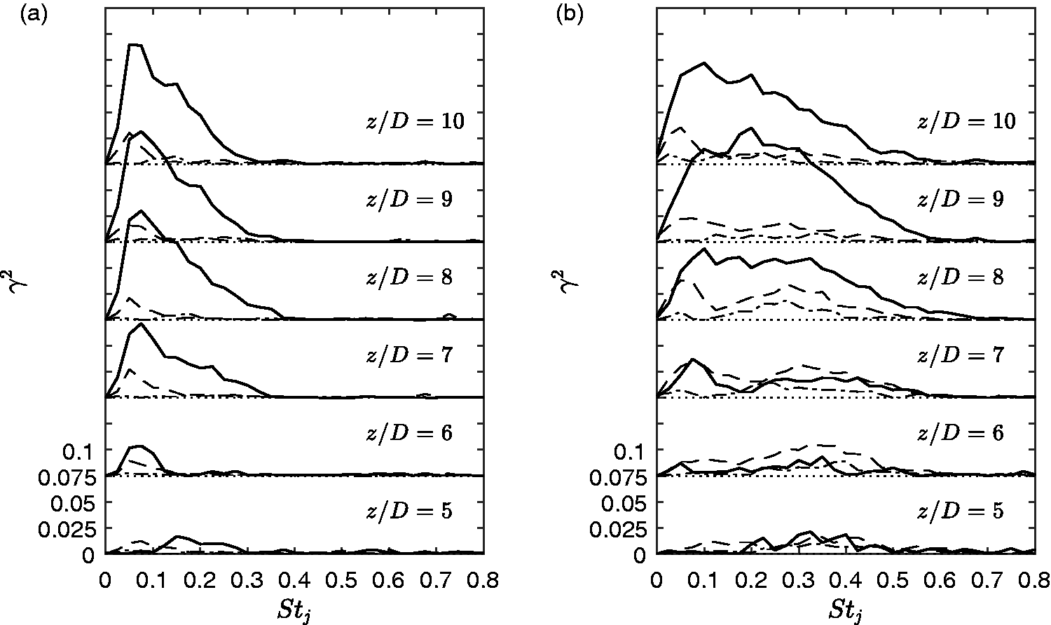
The coherence between flow density fluctuations and far-field acoustic pressure measured at different angles is calculated along three lines located at and , for an axial position between and . The coherence spectra found with the microphone are presented in Figure 6. The order of magnitude of appears to be similar for the two jets at first sight. Nevertheless, the distribution of coherence is found narrower for the jet than for the jet. For the subsonic jet, the maximum is reached close to , whereas a significant level of coherence is obtained between and for the supersonic jet, which corresponds to the highest pressure fluctuations recorded in the radiated sound field, as shown in Figure 3. These observations agree well with the experimental results by Panda and Seasholtz13 who observed an even wider coherence for a Mach 1.8 jet. The noise production mechanism related to the low frequency range of the jet noise seems less sensitive to the jet Mach number than the higher frequencies, both jets having almost the same Reynolds number here.
Coherence between the far-field acoustic measured at and density fluctuations measured at the indicated axial location and for — - - - - -y y-·-·-·. (a) , (b) .
The coherence is also found weak on the centreline upstream of the end of the potential core for both jets in Figure 6. The latter takes significant values, above the measurement noise, only in a frequency range centred around for and for , but they remain smaller than the values observed downstream of the end of the potential core.
The coherence level at does not exceed 0.025 for the jet and 0.04 for the jet, values which are lower than on the centreline, but the decrease is less significant for the supersonic jet than the subsonic one. Besides, the coherence is close to zero at for the Mach 0.9 jet, whereas low but still significant values are observed at Mach 1.32. The region of sound production radiating toward low angles appears to be located close to the centreline, and its extent is found larger for the Mach 1.32 jet than for the Mach 0.9 jet.
A larger value of the coherence is observed on the line than on the centreline for the jet at and . This result suggests that the flow structures associated with noise production are initially located in the mixing layer and are then convected towards the centreline downstream of the end of the potential core. This remark is also valid for the jet considering the component at . Two humps of coherence are also measured for the Mach 1.32 jet between and along the line. They are centred around and , and separated by a low level close to , that is the Strouhal of maximum far-field pressure fluctuations.
The coherence between density on the centreline and 30° microphone signals is averaged over bandwidths of width 0.1 for Strouhal numbers from to . The axial evolution of this averaged value is presented in Figure 7. Except for the component at Mach 0.9 that is stable downstream , the level of coherence follows the distribution of given in Figure 4.
Evolution along the jet axis of the spectral coherence for an observer located at . (a) , (b) .
Finally, the evolution of the coherence as a function of the microphone angle is analysed in Figure 8. The coherence is measured between the acoustic far-field and the density for a probed volume located at and y = 0, that is a point where the coherence is found significant for both jets. A sharp decrease can be seen between and , which is consistent with the results obtained by Panda et al.7
Coherence between the density measured at and y = 0, and the acoustic far-field at the indicated angle θ. (a) , (b) .
This observation also agrees with the feature of noise production by large-scale structures, characterized by its strong directivity in the downstream direction.5,19 Nevertheless, a significant omnidirectional coherence is found for a Strouhal number between 0.05 and 0.1 for the Mach 0.9 jet, and for a small interval for the Mach 1.32 jet. This latter case exhibits a noticeable coherence between Strouhal 0.2 and 0.3 for polar angles up to that is not observed for the subsonic jet. Similar experimental data have been examined for and , but are not presented here since the coherence is almost zero for polar angles greater than .
Density conditional average
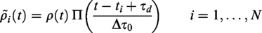
In this section, conditional averages of the density inside the jet flow are computed from far-field pressure events. The aim is to depict the features of turbulent structures that produce a significant part of the radiated acoustic power. The methodology is not new, in particular to highlight the role of large-scale coherent structures in jet noise, using hot-wire anenometry,3 schlieren visualisation20 and infrared radiometry2 to mention a few approaches. The conditional sampling is here based on the fluctuating density measured by Rayleigh scattering, and two types of events are considered, namely minima and maxima of the far-field acoustic pressure signal that exceed a given threshold. The procedure to obtain the density signature is the following. First, the pressure signal is low-pass filtered with a cut-off frequency at Stj = 2. The acoustic events are then identified in the pressure record, leading to N time segments of length for the density
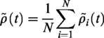
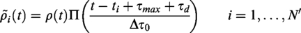
where Π is the rectangular function defined inside the interval and centred around the acoustical time delay ms between the microphone and the probed volume. A preliminary conditional average of the density is then computed as
A jitter may exist between the different individual realisations of induced by random fine-scale turbulence on the evolution of coherent structures. Moreover, some identified events in the acoustic field may not be related to the same acoustic radiation phenomenon. Consequently, this average is affected by different types of smoothing. In order to reduce jittering caused by turbulence, and also to reject possible spurious events, a second step described in Hussain21 is applied. Before the average is calculated, the cross-correlation between and is computed. If the peak of the normalized correlation is lower than 0.2, the realization is rejected. On the contrary, if the peak is higher than 0.2, and if the time lag τmax corresponding to the correlation peak remains smaller than 0.1 ms, the event is stored and re-centred in the time window
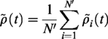
The final conditional average is then estimated from the retained events
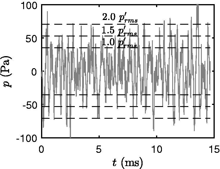
The influence of the threshold value on the results is tested for three different levels equal to 1 , 1.5 and 2. An example of pressure signal is shown in Figure 9. Only high-amplitude peaks, negative and positive, are selected by choosing 2 as the threshold value. In contrast, many spurious events might be identified by taking 1. The amplitude of the conditionally averaged pressure is shown in Figure 10. The average positive or negative events are similar in shape and in amplitude but of opposite sign. The amplitude of the peak rises with the threshold level, which is expected since the average amplitude of the peaks above the threshold rises as well. In order to assess the methodology, in particular the effect of the threshold value applied to the pressure signal, two radial positions are considered for the Mach 1.32 jet at , on the centreline at in a region of low coherence, and at where the coherence takes high values. The results are shown in Figure 11. The density signature does not appear to be affected by the threshold level for both locations, whether for negative or positive pressure events. This observation suggests that the amplitude of the radiated acoustic wave is not directly related with the strength of the identified turbulent event. The threshold is finally arbitrarily set to 1.5 .
Pressure signal measured at for the jet.
Conditional average of the acoustic pressure at for the jet for the indicated threshold applied to the local maxima (a) and minima (b).
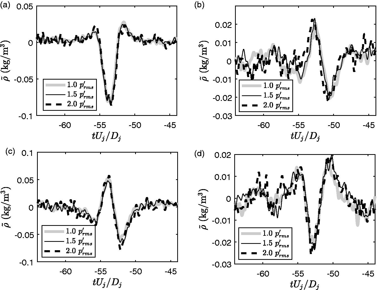
Conditional average of the density based on the local maxima ((a) and (b)) and minima ((c) and (d)) of the acoustic pressure measured at 30° for the thresholds indicated in the graphs. and (a) and (c) y = 0, (b) and (d) .
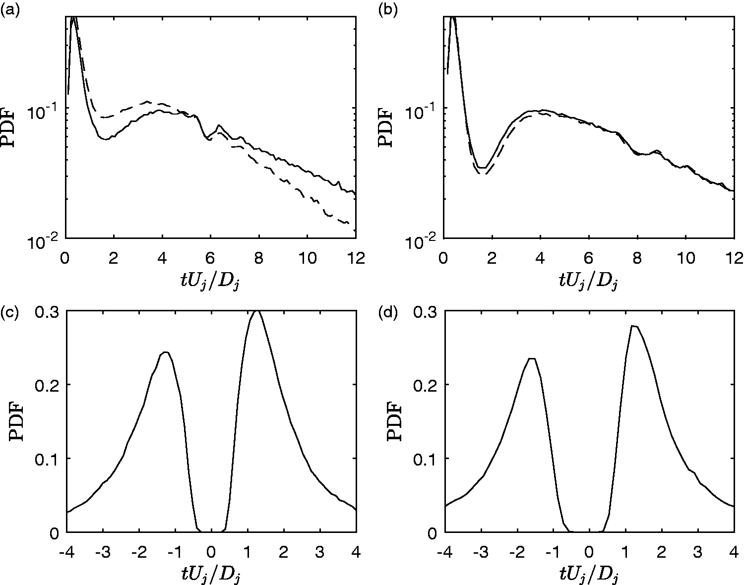
The delay between two consecutive events in the far-field pressure measured at 30° is now studied. The probability density function of this delay is shown in Figure 12(a) and (b). A maximum probability is found close to which corresponds to a Strouhal number , that is slightly above to the cut-off frequency of the low-pass filter. The events associated with these short delays correspond to local extrema that result from the superposition of the high-frequency part of the pressure signal on the lower frequency and high-amplitude pressure events that are of interest in this study. These events are not related with a physical phenomenon in particular. For longer delays, the probability density function forms a hump that is maximum around . The maximum probability is thus found at , which is close to the centre frequency of acoustic spectra for .
(a) and (b) Probability density function (PDF) of the delay between two successive positive (—) and negative () pressure peaks. (c) and (d) Probability density function of the delay between a positive peak and the closest negative peak. (a) to (c) ; (b) to (d) .
The probability density function of the delay between a positive event and the closest negative one is illustrated in Figures 12(c) and (d). The results obtained for both jets are similar and are made of two peaks, one in the negative time delays and a second in the positives. The presence of spikes instead of a flat distribution indicates that positive and negative pressure peaks associated events are not randomly detected. On the contrary, positive events are separated from the closest negative event by a preferential time delay for the jet and for the jet. This delay corresponds with the half-width of the average event shown in Figure 9. All these remarks provide strong evidences that the detected events are related with the dominant contribution to the acoustic pressure at , namely the large-scale noise component. Therefore, they constitute a reliable time reference for studying the source of this noise component by conditional averaging.
Finally, the signatures of the conditional sampling are presented for the criterion based on pressure minima in Figure 13(b) and (d) and on pressure maxima in Figure 13(a) and (c). The results based on pressure maxima exhibit very similar characteristics for the two jet Mach numbers. First, by looking at the centreline, the structure starts being captured at the end of the potential core and grows down to for the jet and for the jet, and then decays. The signal resulting from the average is mostly a deficit of density in the order of 40% of . This value is in the order of the density fluctuations shown in Figure 4, which indicates that such an event at the potential core end is a major contributor to . The duration of the deficit is approximately 0.4 ms for the susbonic jet, and 0.3 ms for the supersonic jet, corresponding to a length of and , respectively, in assuming the turbulence is frozen and the convective velocity is equal to . The density at the trailing edge, that is the right part of the time traces of the structures in Figure 13(a) and (c), corresponds to a hump in density whose amplitude increases with the axial location z/D.
Conditional average of the normalized density at the indicated location, based on the 30° microphone. (a) positive peaks, (b) negative peaks, (c) positive peaks, (d) negative peaks. , , . ⊕ free space propagation delay.
The signals obtained at are very similar in shape with those on the centreline. Nevertheless, they also present a strong deficit of density upstream of the end of the potential core, but the structure strength decays downstream of for both jets. This indicates that the structure was initially convected inside the mixing layer before being transported toward the centre of the jet as it was observed with coherence.
The results obtained along are different firstly because their amplitudes are fairly constant across the considered range of axial locations, and secondly because the structure seems to be out of phase in comparison with the inner part of the jet. Further measurements performed at intermediate radial locations and are now considered to help in interpreting this pattern. The radial evolution of at these axial locations is presented in Figure 14. The cross-correlation function is also shown for completeness. At , the structure can be tracked across the mixing layer. The structure is in advance of approximately 0.08 ms at in comparison to the position . The pattern observed at is the same as at with a time shifting that corresponds to the convection of the structure. This delay is expected to be 0.07 ms for a convective velocity of . There is no clear explanation whether the shape of the profile at has evolved between and , or if the hump visible at –4.9 ms at is the same as the one observed at –5.3 ms at . In the latter hypothesis, that would imply that the local speed of convection is 50 , that is .
Conditional average of the normalized density at the indicated radial location based on the positive pressure peaks from the microphone for the jet. (a) , (b) . Arbitrarily scaled cross-correlation function. Dashed lines in (b) correspond to the solid lines in (a) (See colour version of this figure online). International Journal of Aeroacoustics
Figure 13 (b) and (d) refer to the results associated with the minima of pressure events. The growth and decay of the structure are very similar to what is observed for pressure maxima. The amplitudes are also similar, but the density profiles associated with minima of pressure are found more symmetrical than for maxima, and with a reversed sign.
Concluding remarks
A new experimental setup involving a Rayleigh scattering-based method has been installed in a large anechoic wind tunnel to investigate mixing noise generation mechanisms. Two different jets have been considered, a subsonic jet at Mach number and Reynolds number , and a perfectly expanded supersonic jet at and . Two-point statistics built on the far-field acoustic pressure and on the density fluctuations have proved to be valuable indicators to characterize turbulent events linked to the noise emission in the jet downstream direction. This first study has been carried out with the use of a single photomultiplier for Rayleigh scattering measurements, but it has been shown that the shot noise can be removed thanks to an original signal processing.
Footnotes
Authors’ note
This work was performed within the framework of the Labex CeLyA of Université de Lyon, within the program “Investissements d’Avenir” (ANR-10-LABX-0060/ANR-11-IDEX-0007) operated by the French National Research Agency (ANR).
Declaration of conflicting interests
The author(s) declared no potential conflicts of interest with respect to the research, authorship, and/or publication of this article.
Funding
The author(s) disclosed receipt of the following financial support for the research, authorship and/or publication of this article: This work was partially supported by the industrial Chair ADOPSYS and co-financed by SAFRAN-SNECMA and ANR (ANR-13-CHIN-0001–01).
References
1.
JuvéDSunyachMComte-BellotG.Intermittency of the noise emission in subsonic cold jets. J Sound Vib1980;
71: 319–332.
2.
DahanCEliasGMaulardJet al.
Coherent structures in the mixing zone of a subsonic hot free jet. J Sound Vib1978;
59: 313–333.
3.
ZamanKBMQHussainAKMF.Natural large-scale structures in the axisymmetric mixing layer. J Fluid Mech1984;
138: 325–351.
4.
HilemanJIThurowBSCaraballoEJet al.
Large-scale structure evolution and sound emission in high-speed jets: real-time visualization with simultaneous acoustic measurements. J Fluid Mech2005;
544: 277–307.
5.
BogeyCBaillyC.An analysis of the correlations between the turbulent flow and the sound pressure fields of subsonic jets. J Fluid Mech2007;
583: 71–97.
6.
Kearney-FischerMSinhaASamimyM.Intermittent nature of subsonic jet noise. AIAA J2013;
51: 1142–1155.
7.
PandaJSeasholtzRElamK.Investigation of noise sources in high-speed jets via correlation measurements. J Fluid Mech2005;
537: 349–385.
8.
AndréBCastelainTBaillyC.Experimental study of flight effects on screech in underexpanded jets. Phys Fluid2011;
23, 126102: 1–14.
9.
MercierBCastelainTBaillyC.Experimental characterisation of the screech feedback loop in underexpanded round jets. J Fluid Mech2017;
824: 202–229.
10.
MercierBJondeauECastelainTet al.
Density fluctuations measurement by Rayleigh scattering using a single-photomultiplier. AIAA J2018;
56: 1310–1316.
PandaJGomezCR. Setting up a Rayleigh measuring system in testing facility. AIAA Paper 2003-1089, 2003.
13.
PandaJSeasholtzR.Experimental investigation of density fluctuations in high-speed jets and correlation with generated noise. J Fluid Mech2002;
450: 97–30.
14.
TamCGolebiowskiMSeinerJ. On the two components of turbulent mixing noise from supersonic jets. AIAA Paper 96-1716, 1996.
15.
TamCKWJacksonJASeinerJM.A multiple-scales model of the shock-cell structure of imperfectly expanded supersonic jets. J Fluid Mech1985;
153: 123–149. DOI:10.1017/S0022112085001173.
16.
FuchsHV.Measurement of pressure fluctuations within subsonic turbulent jets. J Sound Vib1972;
22: 361–378.
17.
TowneACavalieriAVJordanPet al.
Acoustic resonance in the potential core of subsonic jets. J Fluid Mech2017;
825: 1113–1152.
18.
KerhervéFPowerOFitzpatrickJet al. Determination of turbulent scales in subsonic and supersonic jets from LDV measurements. In: 12th international symposium of applications of laser techniques to fluid mechanics paper 12.2,2004.
19.
TamCViswanathanKAhujaKet al.
The sources of jet noise: experimental evidence. J Fluid Mech2008;
615: 253–292.
20.
MooreCJ.The role of shear-layer instability waves in jet exhaust noise. J Fluid Mech1977;
80: 321–367.
21.
HussainAKMF.Coherent structures and turbulence. J Fluid Mech1986;
173: 303–356.