A numerical study of an acoustic–hydrodynamic system exhibiting an intermittent prelude to instability

Abstract

A model problem comprising two subsytems (acoustic and hydrodynamic), both admitting unsteady flows, has been studied using numerical simulations. Simulations capture all key features observed in an experiment with a similar configuration, and reveal the differences in flow field evolution that manifest as an intermittent prelude to instability in this nonlinear system, coupling acoustic and hydrodynamic phenomena. The system consists of a uniform flow that enters a long duct and leaves through an orifice into the atmosphere. The duct supports acoustic modes, while the shear layer at the boundary of the jet emerging from the orifice can develop into a train of vortices. Over some range of inflow velocities that support a stable operation, duct acoustic modes and shear layer breakup result in aperiodic, small amplitude pressure fluctuations. As the flow rate is increased, fluctuations become essentially periodic and have much larger amplitudes. This transition from a quiescent to a (so-called) whistling state occurs over a range of flow rates and is characterized by intermittent, moderately large, aperiodic fluctuations. As in the experiment, the aperiodic time series from the quiescent state is found to be multifractal; multifractality is then lost as the flow transitions to whistling. Simulation flow fields reveal differences in the development of vortices in the bounding shear layer, and near the orifice walls, that give rise to the large changes in pressure fluctuations, as well as the intermittent behavior that precedes whistling.

Keywords

Coupled flow dynamics intermittency multifractal time series

Introduction

Large pressure fluctuations accompanying flow oscillations can cause significant, continuing or catastrophic, structural damage. For example, in aircraft engine combustion chambers, heat release rate fluctuations can cause pressure fluctuations to grow if the heat release rate is in phase with the pressure oscillations. Designs must guard against resonant responses of flows in ducts and pipes.¹ Resonant responses can occur in solid rocket motors. Propellant grains in such motors are terminated by a layer of inert material to prevent the burning of propellant from the sides. Flow past a protrusion of inert material may excite sharp tones due to shed vortices.² These pressure fluctuations change burn rates and the motor goes unstable. Many of these systems have two or more subsystems that can have oscillatory responses. For some range of system parameters, there may be small amplitude fluctuations only. However, outside this range, a stronger response may be obtained due to coupling of two or more subsystems. In this paper, we report such changes in response of a model system with two subsystems, one of which is simple duct acoustics and the other is a shear layer. Over some ranges of a single control parameter (a Reynolds number), the system exhibits low amplitude unsteadiness, which will be termed a quiescent state. As the control parameter is changed, a much stronger response, termed whistling, occurs. It turns out that for a range of values of the control parameter near the value at which whistling occurs, the response level is just slightly larger than that of the quiescent stage, but, more importantly, is intermittent, because the shear layer dynamics is nonlinear.

Typically, excitation of duct or pipe tones requires a sharp edge, an orifice or a cavity, where vortical structures form and get shed, and which are sources of acoustic radiation.^3–5 Many experiments on duct flows with single and double orifice configurations have been reported,^6–10 motivated by their presence in pipelines for measurement or control. Studies of the interaction of acoustic waves with the flow through orifices in ducts have also been performed to understand the damping that can be provided by perforated liners in gas turbine combustors. Rupp et al.¹¹ have studied the damping at a circular orifice in a duct (experiment), while Dai et al.¹² have considered a rectangular slit (numerical study). Anderson conducted an extensive study of sound production in a single orifice configuration.^13–17 He detected pipe tones, and concluded that the source of the acoustic waves for the sustenance of the pipe tone was the orifice at the exit. Pipe tones were particularly sharp when the orifice was sharp-edged rather than round-edged. The pipe-tone frequency shifted from one duct mode to another as flow velocity was increased. Anderson supposed that the boundary layer growing on the orifice wall separated and shed vortices to serve as the source of sound. Shadowgraph visualization showed vortex shedding at the acoustic frequency. In a similar arrangement, Karthik et al.¹⁸ examined the development of the jet emerging from the orifice. Time-resolved Schlieren images showed periodic shedding to occur at the natural duct-acoustic mode. Downstream, adjacent vortices merged, and fluctuated at half the shedding frequency. When an intense tone was heard, the duct mode frequency coincided with the frequency of the merged vortex.

Recently, Nair and Sujith¹⁹ have studied the response of a configuration comprising a flow through a pipe of length 600 mm and diameter 50 mm terminated by an orifice of diameter 15 mm and thickness 5 mm. The mean velocity of the flow through the orifice was in the range 2.88–4.41 m/s. Pressure signals were recorded with a transducer placed 2 mm from the orifice plate. At a low speed of 2.88 m/s, the pressure signal was aperiodic. As the flow rate increased, their measurements showed intermittent bursts of periodic oscillations amidst epochs of aperiodicity till, at a critical flow rate with mean velocity 4.22 m/s, a “loud and sharp whistling tone” was heard. This is a model configuration of the coupled system, introduced above, in which the long pipe supports acoustic modes and the flow accelerating through the orifice will have a bounding shear layer that can shed vortices.

At the low flow rates in the duct, the acoustic mode frequencies do not change significantly due to changes in the flow rate. The large response occurs when a duct frequency coincides with the most amplified frequency of the shear layer bounding the jet that emerges from the orifice. The most amplified frequency depends on the shear layer thickness. By increasing the flow rate (and Reynolds number), the thickness of the shear layer is reduced till the most amplified frequency coincides with a duct mode frequency. If this were to be a linear problem, there would be an increasing response around this frequency. Since there are nonlinear processes of shear layer roll up and shedding, at nearby Reynolds numbers, there is an intermittent, episodic response. Of course there can be large changes to the shear layer at the orifice which changes the acoustic boundary condition and which can change the duct modes. While we may expect this from our understanding of duct acoustics and shear layer instability, the objective of this numerical study is to obtain the changes to flow structure in the different states, and thereby obtain a mechanistic understanding of the transition to whistling via an intermittent stage. The problem has been formulated to contain essential features of the system in the experiments of Nair and Sujith.¹⁹ While flow visualization in an earlier experiment had suggested some possible changes to flow structure in the emerging jet,¹⁸ the present simulations allow us to identify the changes precisely. Of particular interest is the observation of intermittency preceding the loud whistling response, and the loss of multifractality of the associated time series when the flow loses stability. In the following, the numerical method is discussed briefly, and then data from simulations at three Reynolds numbers that typify quiescent, intermittent and whistling responses are presented. Flow field visualizations in these three modes exhibit qualitative differences in shear layer structure and its development. Time series from these simulations show the loss of multifractality. Further, these results confirm that measures from the intermittent state can serve as indicators of impending instability. Thus, although strong responses have been observed before, and the forecast skill of some properties of time series had also been found, here, the changes to flow structure revealed by the detailed simulations provide a mechanistic understanding of the intermittent route to instability.

Flow configuration

A longitudinal section of the geometry of the simulations is shown in Figure 1. Flow enters a square duct and emerges through a square orifice opening in a flat wall. This is a convenient geometry for the Cartesian grid solver used in this study. The coordinate system is placed such that the duct inlet plane is at x = 0, and the origin is at the center. The orifice thickness l = 0.005 m is the length for non-dimensionalization. The duct length L = 0.1085 m and its cross section was a square of side 0.05 m. The orifice cross section was a square of side w = 0.015 m. Although the reference experiments¹⁹ were carried out with a duct and orifice of circular cross sections, flow development was expected to be qualitatively similar, and found to be so. A second difference is the presence of the wall at the orifice exit in the simulations which cuts off any entraining flow from upstream. The phenomena of quiescent flow, intermittent bursts and whistling were all obtained in these simulations.

Figure 1.

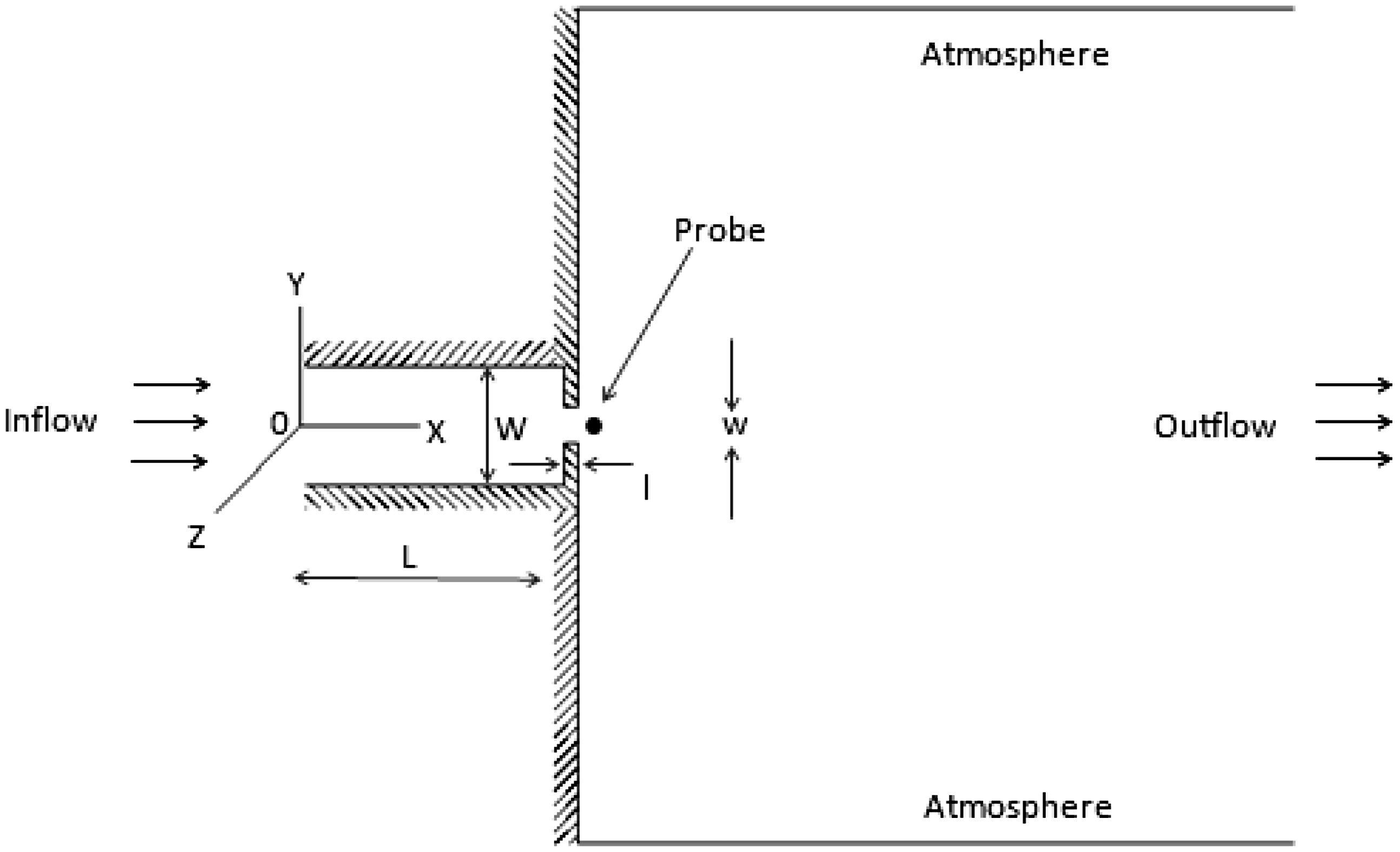
Duct–orifice atmosphere configuration in simulations.

1-D acoustic network analysis

A 1-D linear acoustics solution was obtained by taking the duct and the orifice to be two network elements with interface conditions (matching pressure and mass flow rate). Mean flow was neglected since the mean velocity in the duct (about 1 m/s) was much smaller than the sound speed. In each element, the acoustic pressure and velocity have the forms

p' = A e^{ikx} + B e^{- ikx}, u' = \frac{1}{ρ c_{0}} (A e^{ikx} + B e^{- ikx})

where k is the wavenumber, and x is measured from duct inlet face. Taking duct inlet and orifice exit to be closed, and two matching conditions at the interface, we get the eigenvalue problem

A ϕ = 0

. The matrix

A = (\begin{array}{l} 1100 \\ e^{ikL} e^{- ikL} - e^{ikL} - e^{- ikL} \\ S_{d} S_{d} - S_{o} - S_{o} \\ 00 e^{ik (L + l)} e^{- ik (L + l)} \end{array})

and elements of the eigenfunction

ϕ = (A_{d}, B_{d}, A_{o}, B_{o})

are the amplitudes of the duct and the orifice modes. The frequency

f = c_{o} k / 2 π

. S_d and S_o are cross-sectional areas of duct and orifice, respectively. L and l are duct length and orifice thickness, respectively. Similar problems were solved for other conditions at duct inlet and orifice exit. Frequencies of fundamental and harmonic modes are listed in Table 1.

Table 1.

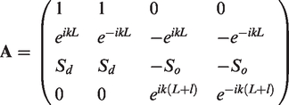
Duct modes computed from the 1-D linear acoustic network analysis.

Inlet condition	Outlet condition	Mode	Frequency Hz
Open	Open	Fundamental	214
Open	Open	First harmonic	471
Open	Closed	Fundamental	145
Open	Closed	First harmonic	436
Closed	Open	Fundamental	95
Closed	Open	First harmonic	335
Closed	Closed	Fundamental	290
Closed	Closed	First harmonic	582

Numerical simulations

Numerical simulations were performed by solving Navier–Stokes equations for compressible flow with an in-house code. Spatial derivatives were computed using an eighth-order compact difference scheme using an equivalent split pair of formulas. This is an extension of a splitting proposed for accurate computation of aeroacoustics.²⁰ The method is suitable for efficient computations (due to good spectral resolution of the high-order compact scheme) of laminar flows, or direct numerical simulations (DNSs) of turbulent flows which resolve all dynamically significant scales. By invoking a high-resolution low-pass filter, large eddy simulations (LESs) of turbulent flows, where only a subrange of the largest scales are resolved, can also be simulated according to the explicit filtering method.²¹ The transport equations were integrated with an explicit, second-order Runge–Kutta method. The original development of the constituent numerical methods and detailed discussions are in Ganesh.²² Enhancements, such as increasing the spatial discretization from fourth to eighth order, and MPI parallelization, are discussed in Kamin.²³ Specific validations of the code were performed by computing the scattering of a pressure pulse that travels to a circular obstacle as in Hixon and Turkel,²⁰ and LES of compressible channel flow at a bulk Reynolds number of 3000 and Mach number of 1.5, for which a benchmark DNS solution is available.²⁴ The scattering problem (2-D) can uncover coding, dispersion, and dissipation errors. The LES problem can help flag more subtle, cumulative errors in a general, nonlinear, 3-D, unsteady flow. Results of these validations are in Kamin.²³ At the conditions of the simulations presented below, even in the jet emerging from the orifice, the flow is unsteady but not turbulent, though it would become turbulent downstream.

Three, clustered Cartesian grids spanned the computational region, one each for the duct, the orifice and the free jet region. Clustering was for resolving the different shear layers—boundary layers on the duct-exit face, the orifice, and the bounding shear layer of the jet. There is no clustering near the duct walls because flow velocities in the duct are very small and duct boundary layer growth has no significant effect on the phenomena studied. Grid sizes were arrived at by performing a sequence of simulations on increasingly finer grids. The results presented below were taken from a grid with the following point distribution. Within the orifice, there were 57 grid points in the two wall-normal directions, very mildly stretched in geometric progression, with a stretching ratio of 1.02. There were 51 uniformly spaced gridpoints in the streamwise direction. Grids were clustered at the duct-orifice and orifice-atmosphere interfaces. Uniform grid spacing is maintained in the streamwise direction within the orifice. In the duct there were 129 gridpoints across and 95 in the streamwise direction. The atmosphere region had 139 points over $- 0.17$ m $<y, z <0.17$ m and 103 streamwise in 0.1135 m $< x < 0.713$ m, of which the first 40 are uniformly spaced and the remaining stretched at 2%. No-slip, isothermal conditions were specified at all walls. At the boundaries of the atmosphere region, characteristic nonreflecting boundary conditions were applied.^25,26 At the duct inflow plane x = 0, the target streamwise velocity component was specified and cross-stream components were set to zero. As a subsonic inflow, the target density was also specified. When characteristic, nonreflecting conditions are applied at inflow, all quantities change slightly, but are prevented from drifting, by applying a weighted correction.²⁷ A buffer layer over a few grid planes near the atmospheric outflow boundary smoothens outgoing vortices so that there is never any significant reverse flow. For the time series analyses below, signals over many periods of the lowest significant frequency were collected to obtain good estimates of the Hurst exponents. Signal length of 0.937s gave 61 periods at 295 Hz. Although the grid used to obtain such long duration data was slightly smaller (crossflow grid spacing was doubled, streamwise spacing increased slightly; about 4.4 times fewer gridpoints in all), all three types of responses (quiescent, intermittent, and whistling) were obtained.

Simulation results

Since the objective of this study is to obtain the different types of flow, quiescent, intermittent and whistling, a sequence of simulations was performed, at many different duct inlet velocities, to detect these conditions. Here, three cases are presented in detail that exhibit these different flow types. The inflow velocity was uniform over a central part and dropped to zero at the duct walls as per a tanh profile. The mean velocity was 0.9 times that at the duct centerline. The Reynolds number is based on the orifice plate thickness, mean velocity within the orifice, air density 1.1748 kg/m³, and viscosity $1.85 \times 10^{- 5}$ m²/s. Flow velocities in the duct are about 1 m/s and about 10 times larger in the orifice. Air temperature was taken to be small so that the sound speed would be small (64 m/s). Then, the maximum Mach number would be about 0.2 (whistling case), there would be no compressibility effects anywhere, and a reasonable time step (limited by sound speed) could be taken. Accordingly, the ambient pressure was 3372 Pa. The simulation was run for 2.5 flow-through times to reach a stationary state before recording pressure signals and field data for analyses. In the following, the pressure signal $p' (t)$ on the central axis ( $y = z = 0$ ) at x = 0.1165 m, which is just downstream of the orifice exit, will indicate the different flow types obtained.

Quiescent flow, Re = 2750

In this case a low-amplitude, aperiodic response was observed. The duct centerline velocity at inflow was 0.3 m/s. Pressure at the duct inlet evolved to 3456.9 Pa. Since the bounding shear layer of the jet that emerges from the orifice is convectively unstable, the presence of small amplitude fluctuations (representing natural perturbations in experiments) are needed to sustain the instability. While numerical errors may suffice, small amplitude random fluctuations with rms of 0.6% of mean were added to the inflow profile of the streamwise component. These are then carried by the flow to the emerging shear layer. A segment of the fluctuating pressure at the probe, located just downstream of the orifice exit (Figure 1), is shown in Figure 2(a). Its Fourier transform (Figure 2(b)) shows peaks at 94 Hz, 290 Hz, 580 Hz, and a smaller one beyond 800 Hz. From the results of the 1-d acoustic model in Table 1, these peaks are the fundamental mode for closed-open, and fundamental and first harmonic for closed–closed boundary conditions, respectively. At the inflow plane, velocity is held fixed while the pressure fluctuates as acoustic waves are allowed to leave the inflow boundary; so “closed” is the correct condition at inflow. At the orifice exit, the open condition corresponds to pressure being held fixed (atmosphere). The higher frequencies correspond to the orifice exit being an acoustically closed boundary. The flow is essentially laminar. The jet that emerges from the nozzle does not breakdown to turbulence and does not have a broadband spectrum. The aperiodic low-amplitude fluctuations are a combination of the duct modes (tonal) and the weak response of the shear layer to the low-amplitude, random perturbations at the duct inflow.

Figure 2.

Pressure signal and spectrum, Re = 2750. (a) Pressure fluctuation $p' (t)$ at the probe location. (b) Magnitude of Fourier transform of $p' (t)$ .

A visualization in terms of spanwise vorticity on the central z = 0 plane is shown in Figure 3. As the flow accelerates along the duct endwall toward the orifice, vorticity levels increase. Unable to negotiate the 90° turn, flow separates at the orifice lip but reattaches just upstream of the orifice exit (see streamlines in Figure 3(b)). The very low amplitude pressure fluctuations are accompanied by very low amplitude changes to the flow structure seen in Figure 3. In particular, there is no roll up or breakup of the shear layer.

Figure 3.

Laminar shear layer emerging from orifice and recirculation zone on orifice wall, Re = 2750. (a) Vorticity (1/s) component ω_z on plane z = 0. (b) Streamlines and streamwise velocity (m/s) field.

Intermittent stage, Re = 8850

Until inlet velocity was increased sufficiently for the onset of whistling, the amplitude of pressure fluctuations did not increase significantly. Intermittent bursts, amidst epochs of weaker aperiodic fluctuations, appeared in the pressure signal as the Reynolds number was increased, as in the intermittent regime of the experiments.¹⁹ The pressure signal shown in Figure 4(a) is remarkably similar in appearance to that found in the experiment. The mean inflow velocity was 1.0 m/s; rms of added fluctuations was 2.2%. The Fourier transform has a broad peak beginning a little above 200 Hz, and smaller amplitudes till about 500 Hz (Figure 4(b)). There is no clear match with any acoustic mode listed in Table 1.

Figure 4.

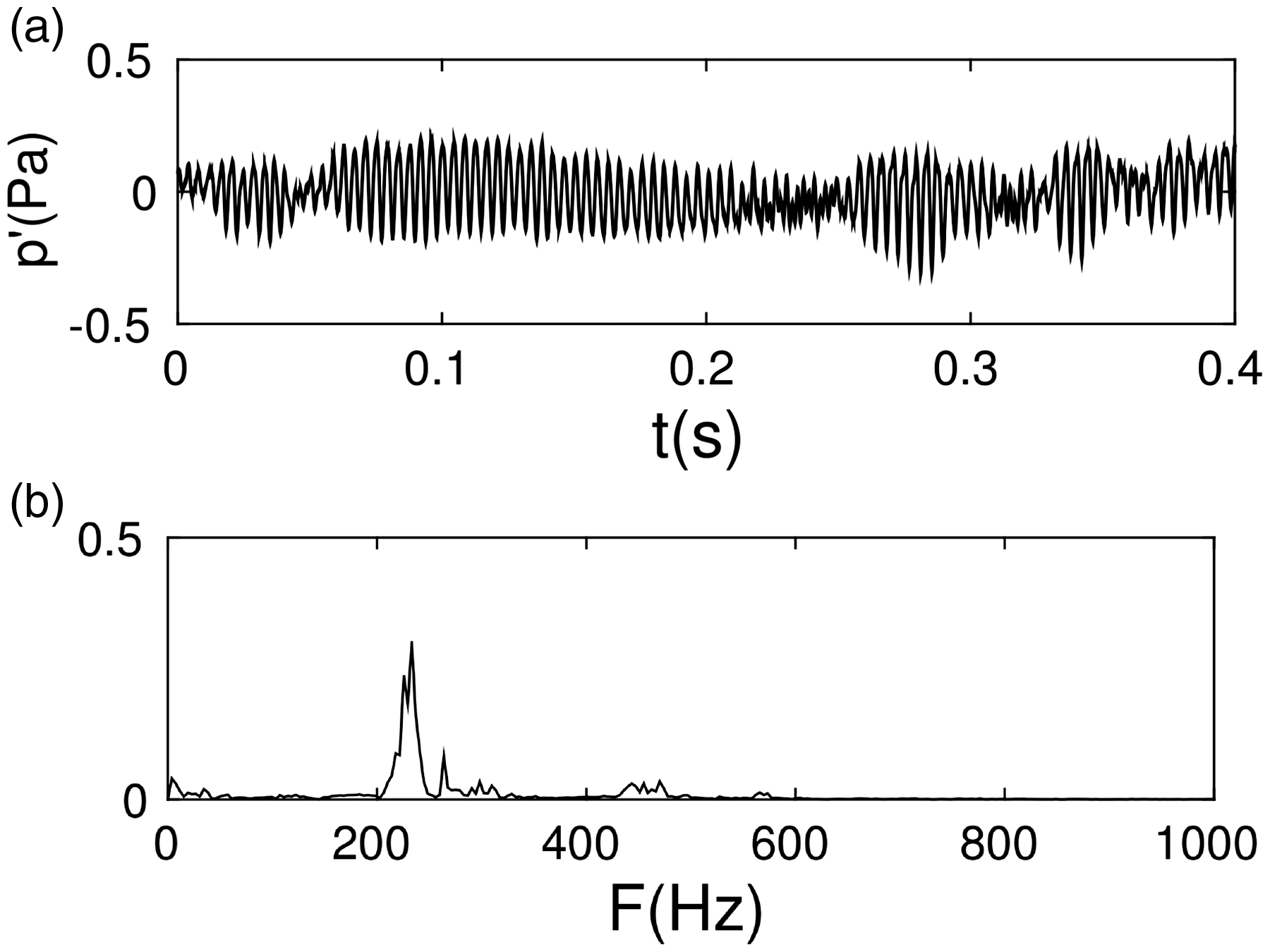
Pressure signal and spectrum, Re = 8850. (a) Pressure fluctuation $p' (t)$ at the probe location. (b) Magnitude of Fourier transform of $p' (t)$ .

Vorticity fields on z = 0 in Figure 5 at two instants show breakup of the shear layer bounding the jet. Such a breakup was not observed at the lower Reynolds number. As will be seen below, at whistling the breakup is more pronounced and a train of vortices appear. The slightly higher level of inflow fluctuations was needed to obtain a significant amplitude of the intermittent bursts. Since the origin of these bursts is the growth of linear instability waves on the jet’s bounding shear layer, a larger perturbation results in a larger amplitude of these waves. Clearly, the intermittent response owes to the intermittent growth and breakup of the jet shear layer, excited by the random perturbations in the inflow rather than forcing by a duct acoustic mode. On increasing the Reynolds number, the growth of the shear layer became stronger because viscous damping had decreased.

Figure 5.

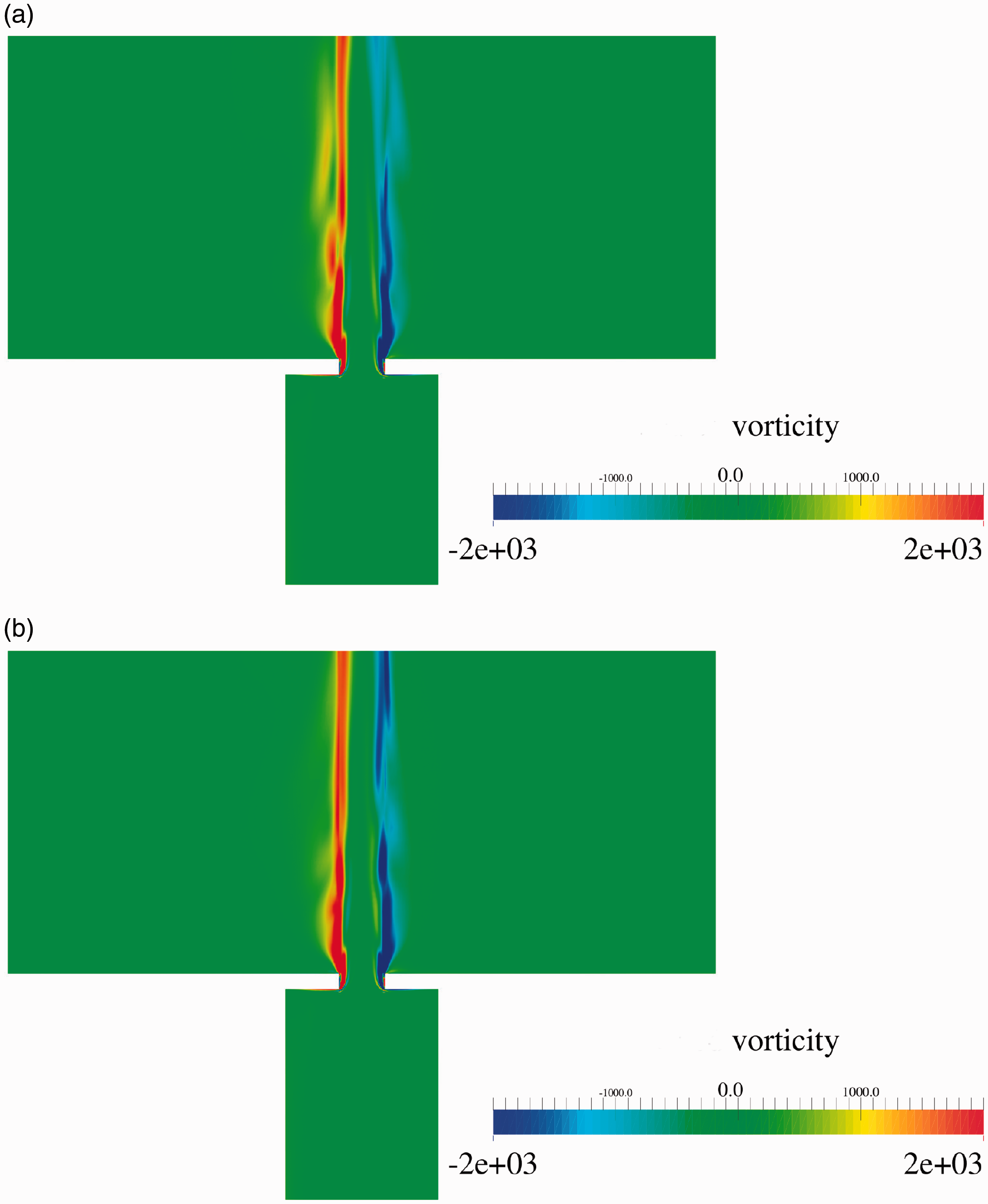
Vorticity (1/s) contours at two instants on z = 0, Re = 8850.

Whistling, Re = 11,500

At inflow velocity of 1.3 m/s, Re = 11,500, “whistling” was observed: the pressure signal was regular and of much larger amplitude, just as in the experiments when whistling was heard.¹⁹ A segment of the time series is shown in Figure 6(a). Its spectrum is a narrow peak at 582 Hz (Figure 6(b)). Velocity fluctuations added to inflow had rms of 0.6% only. The acoustic mode is the first harmonic for closed–closed boundaries (Table 1). The variation of rms of pressure fluctuations along the duct length is shown in Figure 7. 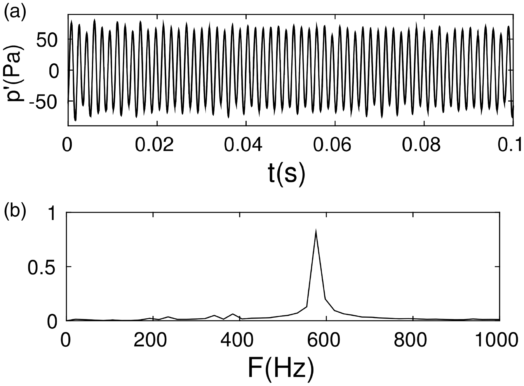The mode shape clearly shows two pressure nodes at $x = L / 3$ and $x = 2 L / 3$ along the duct, and antinodes at the two ends of the duct, modified near the orifice inlet.

Figure 6.

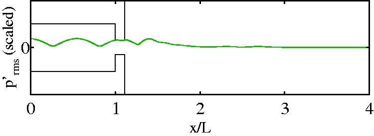
Pressure signal and spectrum, Re = 11,500. (a) Pressure fluctuation $p' (t)$ at the probe location. (b) FFT of the time series.

Figure 7.

Re = 11,500: variation of rms of pressure fluctuation $p_{rms}$ along the flow direction. The maximum value of $p_{rms}$ was 18.6 Pa, found at the centre of the duct. An outline of the duct–orifice configuration has been included in the graph for easy reference.

The changes to flow structure at eight phases $ϕ = nT / 8 (n = 0, 1, \dots 7)$ of one period T, at frequency 580 Hz, can be seen in Figures 8 and 9. At $ϕ = 0$ , the pressure fluctuation $p' (t)$ measured at the probe has its maximum. At this phase, the shear layer that formed on the duct endwall has separated at the orifice lip (Figure 8(a)). The jet becomes thinner as it emerges from the orifice. Its bounding shear layer has rolled up into a vortex. Trailing from this vortex is the upstream shear layer where vorticity is concentrated in two layers. A vortex at the jet boundary that had formed earlier, and had broken off, can be seen. Streamlines in Figure 8(b) show most of the flow to be within the thinning jet. A weak flow at the jet boundary diverges from the jet core as it follows the reattachment near the exit corner of the orifice, and spreads along the outer wall of the orifice plate. The spreading is more pronounced at later phases. The skirt around the jet that had spread over the orifice plate is eventually drawn towards the jet ( $ϕ = T / 2$ ). At $ϕ = T / 8$ , we can observe fluid from the surroundings being drawn in along the plate surface and into the orifice itself.

Figure 8.

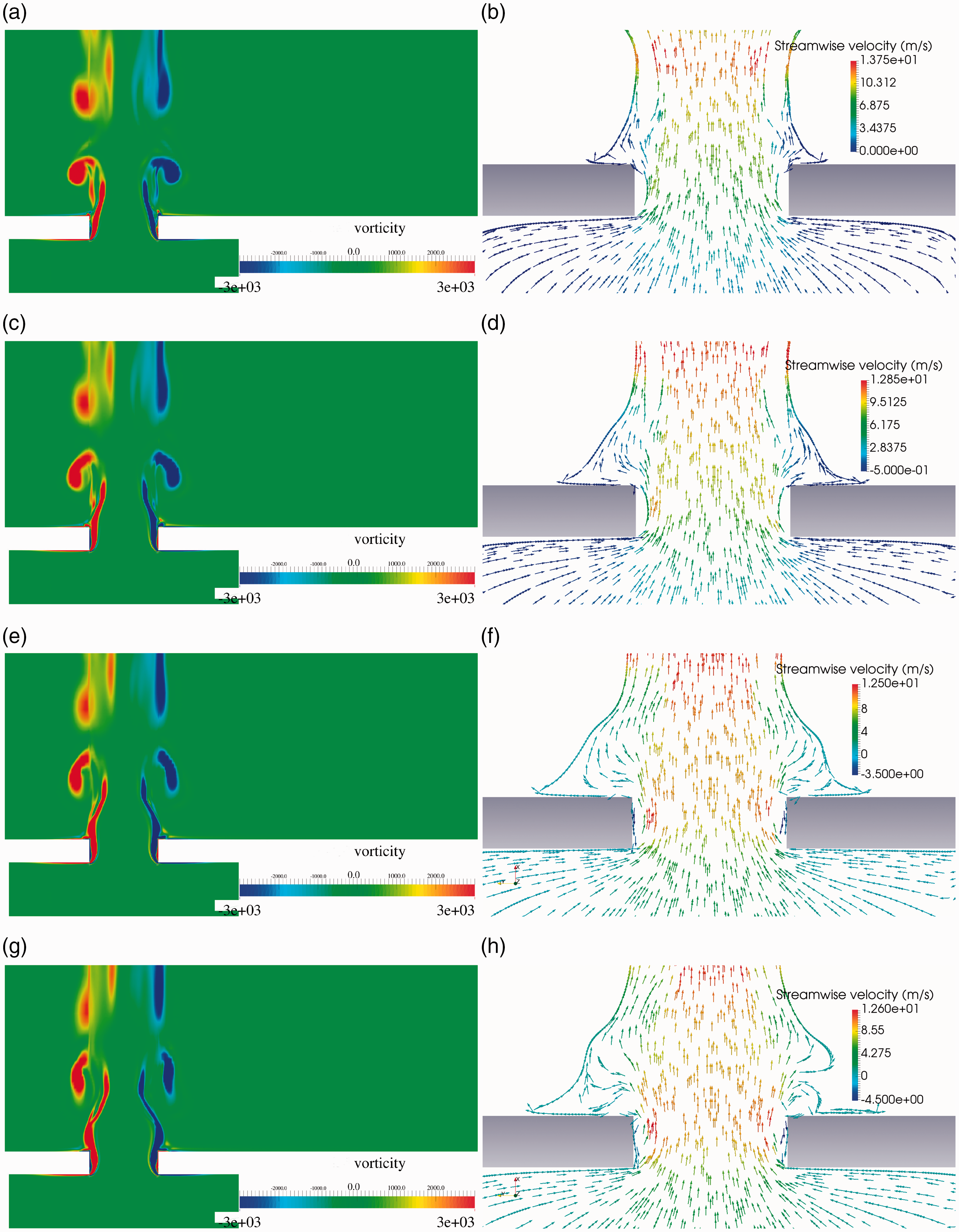
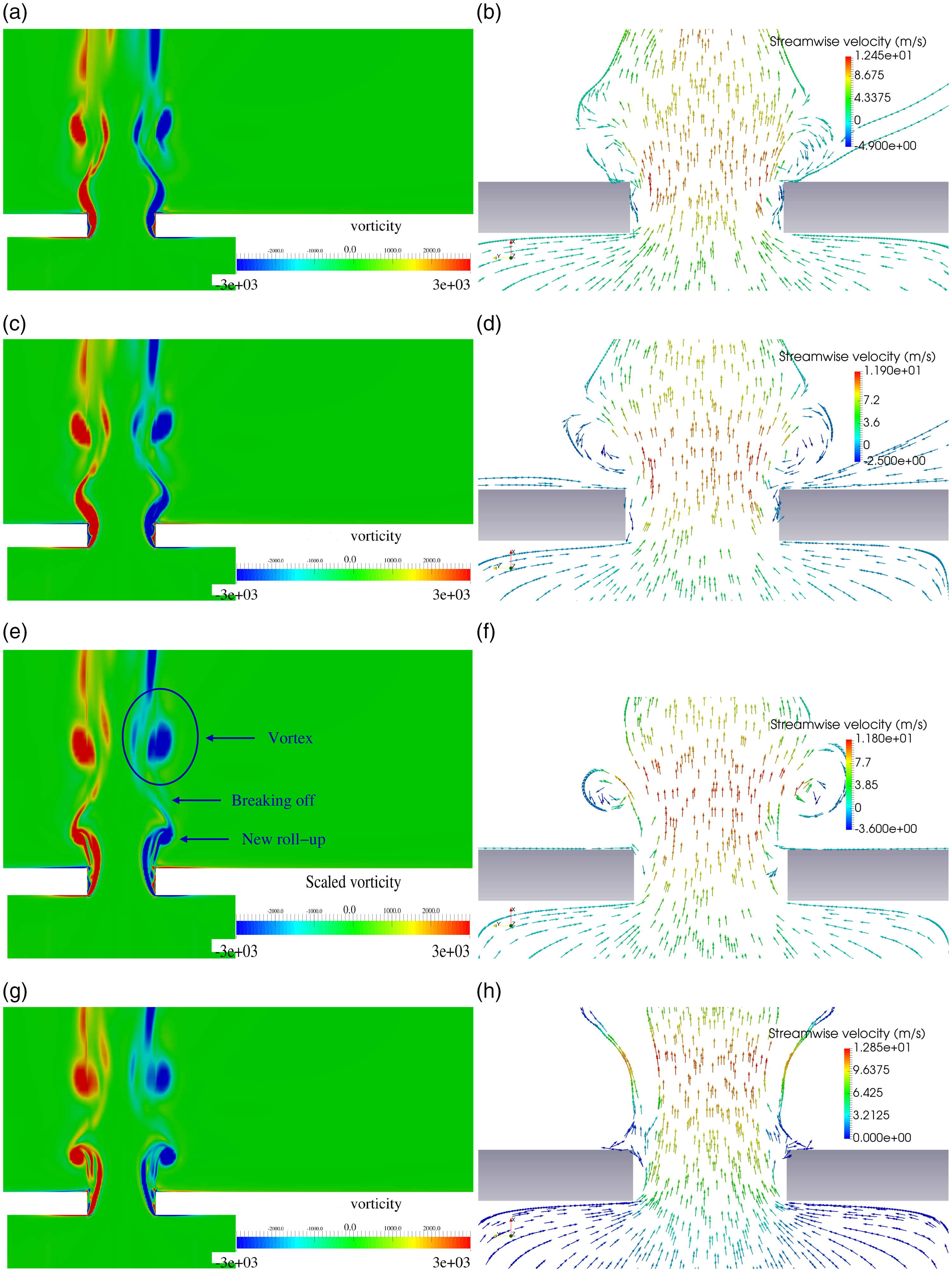
Vorticity (1/s) and quiver plots at phases $ϕ = 0, T / 8, T / 4, 3 T / 8$ , for period T, frequency 580 Hz, Re = 11,500. (a) $ϕ = 0$ . (b) $ϕ = 0$ . (c) $ϕ = T / 8$ . (d) $ϕ = T / 8$ . (e) $ϕ = T / 4$ . (f) $ϕ = T / 4$ . (g) $ϕ = 3 T / 8$ . (h) $ϕ = 3 T / 8$ .

Figure 9.

Vorticity (1/s) and velocity vectors in plane z = 0 at phases $ϕ = T / 2, 5 T / 8, 3 T / 4, 7 T / 8$ , for period T, frequency 580 Hz, Re = 11,500. (a) $ϕ = T / 2$ . (b) $ϕ = T / 2$ . (c) $ϕ = 5 T / 8$ . (d) $ϕ = 5 T / 8$ . (e) $ϕ = 3 T / 4$ . (f) $ϕ = 3 T / 4$ . (g) $ϕ = 7 T / 8$ . (h) $ϕ = 7 T / 8$

In snapshots over $T / 8 \leq ϕ \leq 3 T / 4$ , we observe the formation of a larger vortex structure, but with little vorticity in the core. This larger vortex breaks off around $ϕ = 3 T / 4$ . In the corresponding streamline plots in Figure 8, we can observe the jet change from one that becomes thinner as it emerges, to one that spreads outward as it emerges. Most of the region next to the orifice wall contains a recirculating flow. During the jet’s spreading phase, a thinner neck exists within the orifice ( $ϕ = T / 2, 5 T / 8$ , Figure 9), and flow no longer reattaches within the orifice. After the large vortical structure breaks off ( $5 T / 4 < ϕ < 3 T / 4$ ), a new roll up into the smaller vortex can be seen at $ϕ = 3 T / 4, 7 T / 8$ (marked in Figure 9(e)). Vorticity trailing from this vortex lies in two or three layers. So the jet thins and thickens at this frequency; shear layers from both faces of the orifice plate separate and roll up into a small vortex. It is the continuation of the shear layer roll up into the larger structure, and its break off, that gives rise to the whistling. If the break off had happened after the initial roll up into the smaller vortex, like in many plane mixing layers, the response amplitude would have been smaller. In the intermittent stage discussed above, such a continuing roll up into a large structure was not observed—only the initial roll up and break off.

The significantly larger levels of pressure fluctuations are due to the much larger changes to flow structure in the jet. The roll up into the small vortex, and then into a larger one, accompanies large changes to streamline curvature; consistently, there must be large fluctuations to pressure also. The dynamics of the separating shear layer depends on the thickness of the shear layer, which depends on the Reynolds number. When whistling occurs, the duct acoustic mode frequency locks on to the frequency of the process of shear layer growth and roll-up into a small vortex; the subsequent roll up into the larger vortex and break off sets up conditions for this cycle to repeat. Though the possible duct acoustic modes remain the same, increasing the Reynolds number creates a thin enough separating shear layer that can support this regular periodic evolution, and the large amplitude pressure fluctuations. In comparison, the jet flow shows little change in structure at the lower Reynolds numbers. At slightly lower Reynolds numbers, there are instants when the shear layer thickness admits a fast growth and break off which increases the level of pressure fluctuations. These appear as bursts, but the acoustic forcing never locks on to the instability evolution of the orifice–jet shear layer. The intermittency at nearby lower Reynolds numbers owes to the nonlinear processes of roll up and break off.

Time series analysis

The structure of the time series from the present simulations are remarkably similar in appearance to those obtained in the experiments.¹⁹ It is low amplitude, aperiodic when the flow is quiescent, has intermittent bursts of slightly larger amplitudes as the flow rate is increased, and is regular when whistling occurs. Analyses developed for fractal time series can provide useful quantitative characterizations that are qualitatively different from classical ones such as moments, correlations and power spectra. The time series of an orderly state such as the regular periodic whistling flow is not fractal, whereas aperiodic ones are multifractal. The procedures, called detrended fluctuation analysis (DFA),²⁸ have been described by Kantelhardt et al.,²⁹ and by Ihlen³⁰ who has also provided implementations as MATLAB codes.

Briefly, first, from a time series $X (t_{i})$ at times t_i, cumulative sums of deviations from the mean of X are calculated. Next, for segments of length s, polynomial fits are found. For each segment of length s, variances F(s) of each segment provide qth-order fluctuation functions $F_{q} (s)$ that are expected to vary as $s^{h (q)}$ . The exponent $h (q = 2) = H$ is the Hurst exponent,³¹ and h(q) is the generalized Hurst exponent. Changes to the Hurst exponent H have been found to be useful as a prognostic of system dynamics which changes from a quiescent to a strong response via an intermittent stage. Secondly, the generalized Hurst exponent is related to the singularity spectrum

f (α) = q (α - h) + 1

(1)

where

α = h + q d h / d q

. For a monofractal signal, h is independent of q and

f (α) = 1

. Characterizations of system responses provided by these quantities will be discussed below along with results.

Hurst exponent

A fractal time series admits the scaling $X (t) = c^{H} X (ct)$ where H is the Hurst exponent. H lies between 0 and 0.5 for an anti-persistent time series and between 0.5 and 1 for a persistent time series. A persistent time series is one for which, on the average, an increase in value is followed by an increase, and a decrease by a decrease. This is indicative of a memory of recent events and slow changes. For an anti-persistent signal, as an increase is followed by a decrease, values tend to return to the series mean. Hurst exponents were calculated from time series of pressure just downstream of the orifice (probe location in Figure 1) at the different conditions, and for a synthetic white noise signal. Signals are shown in Figures 2(a), 4(a), and 6(a). The average of fluctuation functions $F_{q} (s)$ was found over many segments of length s, and segment length was varied between one and four times the period of the lowest significant frequency (290 Hz).

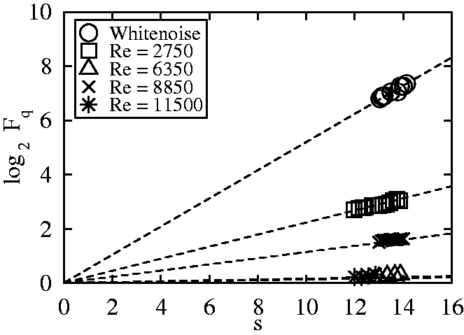
Figure 10 shows the variation of the q-order fluctuation function $F_{q} (s)$ for q = 2 over a range of scales (segment lengths) s. The slopes of the lines on the log–log graph are the values of H. For white noise, the procedure gives H = 0.52, which is close to the theoretical value of 0.5. As the Reynolds number increases and the flow response changes from quiescent (Re = 2750, H = 0.223), intermittent (Re = 8850, H = 0.114) to whistling (Re = 11500, H = 0.016), H decreases to zero. Though not discussed above, whistling was obtained at Re = 6350 also, with H = 0.013. As the flow approaches whistling, H tends to zero, as it should, since H = 0 for a periodic signal. Similar trends were identified in Nair and Sujith¹⁹ for pressure signals from experiments: they found H to lie in the range 0–0.5, and to tend to zero when whistling occurred.

Figure 10.

Hurst exponent H from pressure time series at different Reynolds numbers, and for white noise. (a) White noise. (b) Re = 2750. (c) Re = 8850. (d) Re = 11,500.

For general q, the fluctuation function $F_{q} (s)$ is weighted towards large and small amplitude fluctuations for positive and negative q, respectively. Figure 11 shows the variations of $F_{q} (s)$ for $q = - 3, - 1, 1, 3$ for a range of scales s. The slopes are essentially the same for white noise and when whistling occurs. Changing slopes for Re = 2750 and 8850 indicates multifractality. In Figure 12, these changes in the singularity spectra $f (α)$ (equation (1)) can be observed. $f (α) \approx 1$ at $α \approx 0.5$ for white noise and at $α = 0.5$ for whistling. At other conditions, the signal is multifractal. Again, these results are as in the experiments of Nair and Sujith.¹⁹ The broad spectra at Re = 2750 and 8850 implies a range of temporally varying trends in the time series. The regular signal at whistling collapses the spectrum to a point.

Figure 11.

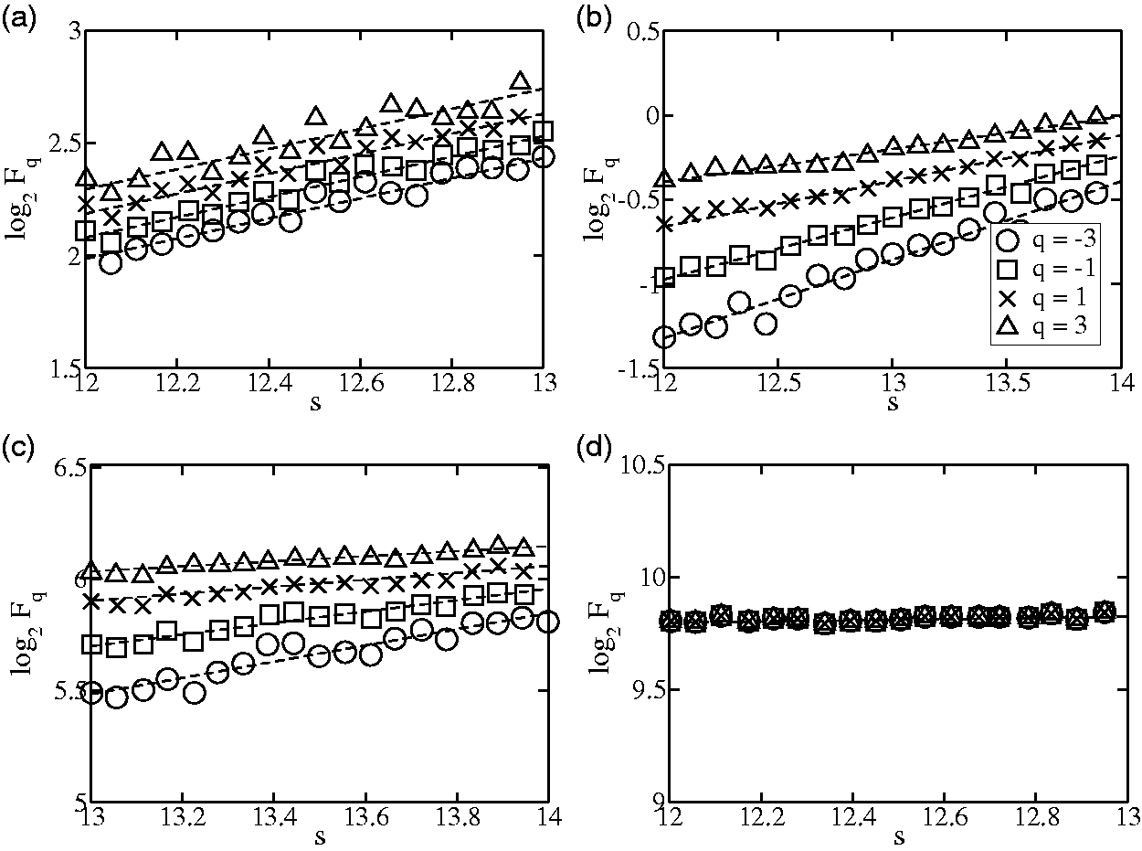
Variation of the Hurst exponent with q order rms. Such a variation is an indicator of multifractality of a signal. As seen here, white noise has a different behavior compared to signals obtained from the simulations in that the slopes of the lines are not q order dependent.

Figure 12.

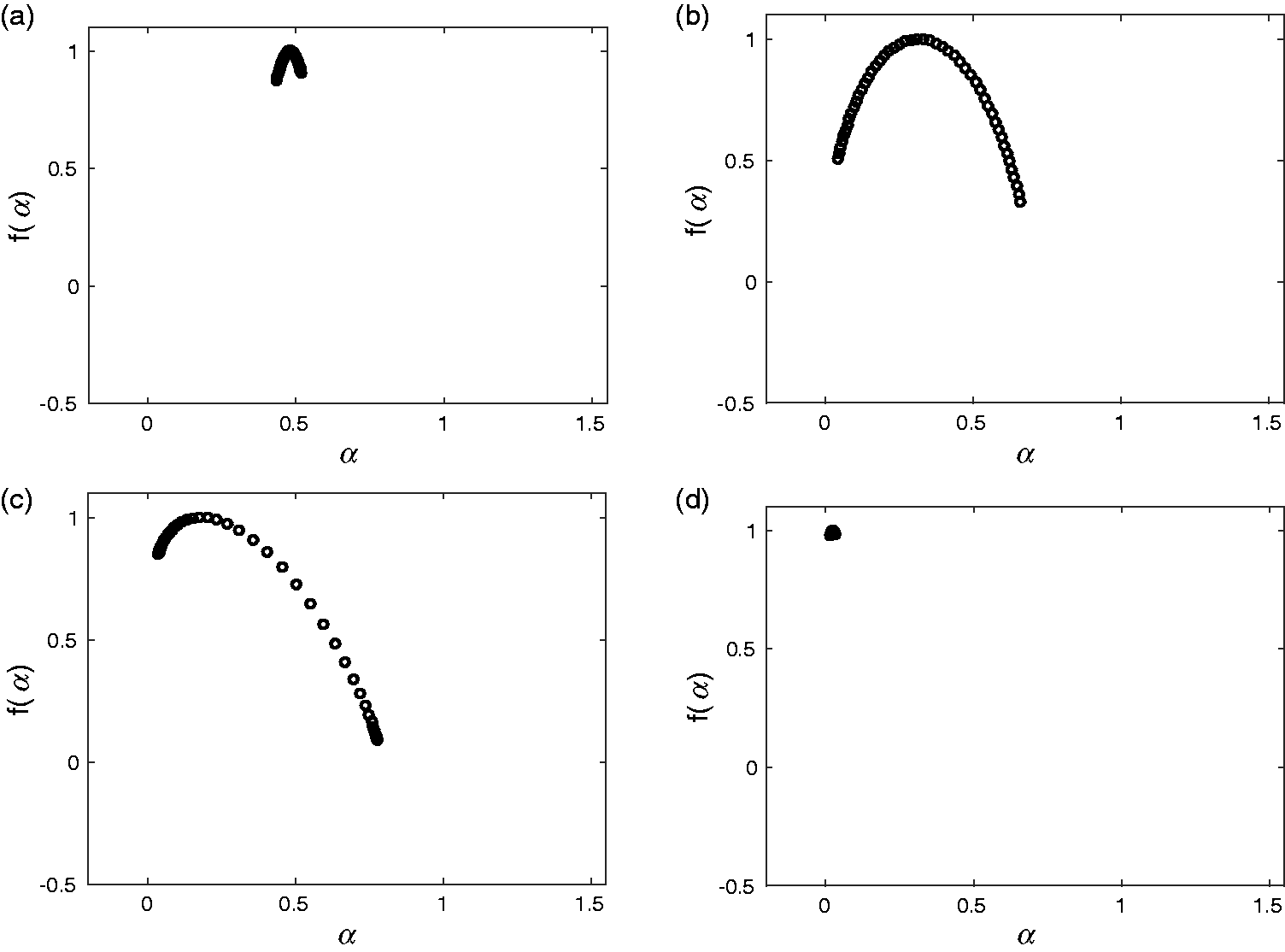
Variation of the structure function $f (α)$ with α showing varying degree of multifractality. The width of the spectrum of $f (α)$ represents the degree of multifractality of the signal. (a) White noise. (b) Re = 2750. (c) Re = 8850. (d) Re = 11,500.

The change in multifractality of the time series can be connected to the structure of the flow in the different states. During stable operation (quiescent), the flow has multiple spatial and temporal scales that contribute to its dynamics, since it responds to noise although with small amplitudes. Hence the pressure fluctuations display multifractality. On the contrary, aeroacoustic instability (whistling) is characterized by a regular large amplitude signal with a single, dominant temporal scale. As a consequence, multifractality is lost with the onset of whistling. Since the onset is via an intermittent route, the loss of multifractality is gradual.

Conclusion

A system comprising a long duct open at one end and terminated by an orifice through which a jet emerges into the atmosphere has been simulated. The configuration is similar to one that had been designed for an experiment to create a coupled acoustic–hydrodynamic system.¹⁹ Simulations at different Reynolds numbers showed system responses characterized as quiescent, intermittent, and whistling. The amplitude of pressure fluctuations was much higher when whistling occurred. An examination of the flow fields revealed that in the quiescent state a shear layer separates at the upstream end of the orifice and reattached within it, and thereafter develops slowly along the jet boundary. In the intermittent stage, this shear layer breaks up intermittently. When whistling occurs, there are large and very nearly periodic changes in the development of the emerging shear layer. At some phase in the response, the shear layer rolls up into a small vortex. Subsequently, this evolves into a larger vortex, which then breaks off and sets up conditions for the cycle to repeat. The flow is more complex due to the periodic growth of a skirt around the jet that spreads over the outer wall of the orifice plate over a part of the cycle. Over the subsequent part of the cycle, the skirt is drawn toward the jet and a flow develops along the plate which enters the orifice. Thus, the response is more complex than, say, a simple instability of the emerging shear layer. During whistling, the strong shear layer dynamics is organized by the duct acoustic mode, whereas in the quiescent stage, there is but a weak modulation of the shear layer development. Owing to the nonlinear processes of shear layer roll up and break off, at nearby Reynolds numbers, the forcing from the duct acoustic mode occasionally excites a break off and results in an intermittent burst. A Fourier transform of the signal does not show any significant content at the duct–acoustic frequency.

Besides this, mechanistic picture of the flow features revealed by the simulation, time series of the evolution exhibit features and changes found in the experiment; especially, the appearance of bursts separated by epochs of weaker fluctuations in the intermittent regime. As the flow transitions from quiescent to intermittent flow, the Hurst exponent drops from about 0.223 to 0.114, and then to 0.016 at whistling. There is also a loss of multifractality during this transition.

The simulations demonstrate that the intermittent route to transition is more generic, and not merely a feature of the specific experiment. Though the square cross section of the duct and orifice were convenient for the code used, the close connection between the present results and those of the experiment with a circular pipe and orifice indicate the generality of such system dynamics. Indeed such transitions exhibiting an intermittent precursor stage have been observed at the onset of combustion-driven oscillations,³² at the onset of wing flutter,³³ and surge in a turbocharger compressor.³⁴ The changes to time series properties (Hurst exponent, quantitative; loss of multifractality, qualitative) are also a more sophisticated confirmation of the correctness of numerical methods used for long duration simulations of the Navier–Stokes equations for unsteady, compressible flow.

Footnotes

Declaration of conflicting interests

The author(s) declared no potential conflicts of interest with respect to the research, authorship, and/or publication of this article.

Funding

The author(s) received no financial support for the research, authorship, and/or publication of this article.

References

Bruggeman

Hirschberg

Dongen

MEH

, et al. Self-sustained aero-acoustic pulsations in gas transport systems: experimental study of the influence of closed side branches. J Sound Vib 1991; 150: 371–393.

Vuillot

Vortex shedding phenomena in solid rocket motors. J Prop Power 1995; 11: 626–639.

Powell

On the edge tone. J Acoust Soc Am 1961; 33: 395–409.

Chanaud

Powell

Some experiments concerning the hole and ring tone. J Acoust Soc Am 1965; 37: 902–911.

Rockwell

Naudascher

Review—self-sustaining oscillations of flow past cavities. J Fluids Eng 1978; 100: 152–165.

Culick

FEC

Magiawala

Excitation of acoustic modes in a chamber by vortex shedding. J Sound Vib 1979; 64: 455–457.

Nomoto

Culick

FEC.

An experimental investigation of pure tone generation by vortex shedding in a duct. J Sound Vib 1982; 84: 247–252.

Karthik

Kowsik

BVR

Venkateswarlu

, et al. Acoustic field in a duct resulting from vortex shedding from multiple restrictors. J Aero Sci Tech 2005; 57: 1–8.

Wilson

Beavers

DeCoster

, et al. Experiments on the fluid mechanics of whistling. J Acoust Soc Am 1971; 50: 366–372.

10.

Testud

Aurégan

Moussou

, et al. The whistling potentiality of an orifice in a confined flow using an energetic criterion. J Sound Vib 2009; 325: 769–780.

11.

Rupp

Carrotte

Spencer

Interaction between the acoustic pressure fluctuations and the unsteady flow field through circular holes. J Eng Gas Turb Power 2010; 132: 1–9.

12.

Dai

Jing

Sunx

Acoustic-excited vortex shedding and acoustic nonlinearity at a rectangular slit with bias flow. J Sound Vib 2014; 333: 2713–2727.

13.

Anderson

ABC.

Dependence of pfiefenton (pipe tone) frequency on pipe length, orifice diameter, and gas discharge pressure. J Acoust Soc Am 1952; 24: 675–681.

14.

Anderson

ABC.

Dependence of the primary pfiefenton (pipe tone) frequency on pipe-orifice geometry. J Acoust Soc Am 1953; 25: 541–545.

15.

Anderson

ABC.

A jet-tone orifice number for orifices of small thickness–diameter ratio. J

Acoust Soc Am 1954; 26: 21–25.

16.

Anderson

ABC.

Meta-stable jet-tone states from sharp-edged, circular, pipe- like orifices. J

Acoust Soc Am 1955; 27: 13–21.

17.

Anderson

ABC.

Vortex-ring structure transition in a jet emitting discrete acoustic frequencies. J Acoust

Soc Am 1956; 28: 914–921.

18.

Karthik

Chakravarthy

Sujith

RI.

Mechanism of pipe-tone excitation by flow through an orifice inside a duct. Int J Aeroacoust 2008; 7: 321–348.

19.

Nair

Sujith

RI.

Precursors to self-sustained oscillations in aeroacoustic systems. Int J Aeroacoust 2016; 15: 312–323.

20.

Hixon

Turkel

Compact implicit MacCormack-type schemes with high-accuracy. J Comput Phys 2000; 158: 51–70.

21.

Mathew

Lechner

Foysi

, et al. An explicit filtering method for large eddy simulation of compressible flows. Phys Fluids 2003; 15: 2279–2289.

22.

Ganesh

Large eddy simulation of free and impinging subsonic jets and their sound fields. PhD thesis, Department of Aerospace Engineering, Indian Institute of Science, Bangalore, 2016.

23.

Kamin

A numerical study of changes to flow organization and their prognostic measures. Master’s thesis. Department of Aerospace Engineering, Indian Institute of Science, Bangalore, 2017.

24.

Lechner

Sesterhenn

Friedrich

Turbulent supersonic channel flow. J Turbulence 2001; 2. DOI: 10.1088/1468-5248/2/1/001.

25.

Thomson

KW.

Time dependent boundary conditions for hyperbolic systems. J Comput Phys 1987; 1987: 681–624.

26.

Thomson

KW.

Time dependent boundary conditions for hyperbolic systems, II. J Comput Phys 1990; 1990: 89439–89461.

27.

Bogey

Bailly

Three-dimensional non-reflective boundary conditions for acoustic simulations: far field formulation and validation test cases. Acta Acust 2002; 2002: 88463–88471.

28.

Peng

Buldyrev

Havlin

, et al. Mosaic organization of DNA nucleotides. Phys Rev E Stat Phys Plasmas Fluids Relat Interdiscip Topics 1994; 49: 1685–1689.

29.

Kantelhardt

Zschienger

Koscielny-Bunde

, et al. Multifractal detrended fluctuation analysis of nonstationary time series. Physica A 2002; 316: 87–114.

30.

Ihlen

EAF.

Introduction to multifractal detrended fluctuation analysis in Matlab. Front Physiol 2012; 2012: 3.

31.

Hurst

HE.

Long-term storage capacity of reservoirs. Trans ASCE 1951; 1951: 116770–116799.

32.

Nair

Thampi

Sujith

RI.

Intermittency route to thermoacoustic instability in turbulent combustors.

J Fluid Mech 2014; 756: 470–487.

33.

Venkatramani

Nair

Sujith

, et al. Multi-fractality in aeroelastic response as a precursor to flutter. J Sound Vib 2016; 386: 390–406.

34.

Kerres

Nair

Cronhjort

, et al. Analysis of the turbocharger compressor surge margin using a Hurst-exponent-based criterion. SAE Int J Eng 2016; 9: 1795–1806.