



Abstract
A two-dimensional model of the edge tone is studied by a highly accurate and reliable method of direct numerical simulation of the compressible Navier-Stokes equations, and used to verify key features observed in previous experimental and numerical studies, and to discover new features related to the jet motion and the edge tone generation mechanism. The first and second modes of the edge tone that are numerically reproduced agree well with Brown’s equation. In the mode transition region, dynamical mode transition is observed at a fixed jet velocity. For both first and second modes, the pressure distributions are antisymmetric with respect to the edge plate, and the sound intensity is proportional to the fifth power of the jet velocity. These results are consistent with the edge tone being radiated from a dipole-like source. Spatial profiles of the velocity and the velocity variance of the oscillating jet are also investigated for each mode over a range of the jet velocity including the mode transition regime. The amplitude of the velocity oscillation becomes constant with increasing jet velocity, while a measure of the amplitude of the velocity variance profile, which is introduced to characterize the strength of the jet fluctuation and named the ’fluctuation strength’, is proportional to the third power of the jet velocity. Some properties of the fluctuation strength correspond to properties of the sound intensity, including the first mode having larger amplitude than the second mode, and the way of deviating from the power law at smaller values of jet velocity and in the mode transition region. It is proposed that the third-power law exhibited by behavior of the fluctuation strength could be related to the increase of the skewness observed in the velocity profile with increase of jet velocity, and a model calculation is used to support this proposal.
Introduction
The edge tone is generated from an oscillating jet colliding with an edge and is one of the aerodynamic sounds observed in a low Mach number region.1–3 The elucidation of the mechanism of the edge tone has been a long standing problem in the fields of aeroacoustics, fluid dynamics and acoustics, 2 and its mechanism is not completely understood yet. Furthermore, the study of the edge tone is an important subject in the field of musical acoustics. The edge tone is the sound source of air-jet driven instruments, such as flue organ pipe, flute, recorder, ocarina and shakuhachi, and the study of the edge tone leads us to improving the understanding of the sound mechanism of air-jet driven instruments.4–6
In the long history of study of the edge tone, some important phenomenological and theoretical formulae, which describe basic properties of the edge tone, have been proposed.1,2,7–13 A very useful formula was introduced by Brown 1 based on his experimental results. According to Brown’s formula, the frequency of the edge tone linearly increases with the jet velocity until a mode transition arises. At the mode transition, the hydrodynamic wave of the jet discontinuously changes to a higher mode wave and a change of the tone is observed. The mode transition is hysteretic, that is, the upward and downward transitions follow different paths. The frequencies of individual modes are given by different linear functions of the jet velocity.
The source of the edge tone is the oscillation of the jet colliding with the edge. The jet oscillation is sustained by a feedback cycle: the interaction with the edge induces a feedback to the upstream jet flow emanating from the flue exit. This feedback mechanism has been studied by many authors,7–10,13 Powell introduced a semi-empirical formula for the feedback cycle based on experiments, which he called the irrotational feedback mechanism. 8 Holger et al. developed the formula focusing on the fluid mechanism of the vortex street and predicted the oscillation frequencies.9,10 By using a linear analytical model of the incompressible fluid with the help of a trailing-edge Kutta condition and the Wiener-Hopf method, Crighton obtained an almost fully analytic explanation for the feedback cycle and gave a formula that is similar to Brown’s equation 13
Powell and Holger et al. studied the sound intensity of edge tones experimentally and theoretically.8–10 According to their experiments, the edge tone is generated by a dipole-like source, and the intensity of the edge tone increases according to the 6th-power of the jet velocity (6th-power law) as expected from the theory of aerodynamics sound.2,3 The experiments reported observation of multiple higher modes.1,8 The intensity of each mode of the edge tone obeys a different 6th-power law. 8 Thus, the sound intensity at a given jet velocity depends on the mode selected. Kaykayoglu and Rockwell indicated that a pair of effective pressure sources are located slightly downstream of the edge tip on both sides of the edge plate. 11
In spite of all the above efforts, the generation mechanism of the edge tone has not been adequately explained in terms of the aerodynamics sound theory, yet.2,3,14-16 As an alternative approach, we can rely on numerical methods for compressible fluids, which reproduce the hydrodynamic and acoustic motions simultaneously. In recent years, the edge tone has been numerically studied using several different methods.17–24 Dougherty et al. adopted a compressible fluid simulation and partially reproduced the structure of the mode-transition region. 17 Paál and Vaik reported that the mode transitions of the jet motion are reproduced by an incompressible fluid simulation in a laminar flow regime for a jet with a top-hat inlet profile and the dynamical transition is observed at low Reynolds numbers in the mode transitions region, though the underlying mechanism of the dynamical transition was not explained. 21 The properties of mode transitions change depending on whether the inlet jet velocity profile is a top-hat profile or a parabolic profile, which was also confirmed experimentally. 23 The relationship between the Mach number (jet velocity) and the frequency of the reproduced acoustic wave was discussed in a numerical study with compressible fluid simulations.19,20 A 3 D edge tone was calculated with a hybrid method, which couples a 2 D fluid simulation with a 3 D acoustic simulation. 22 Many types of hybrid methods are widely used for the analysis of aerodynamic sound, because they reduce the computational cost. 25 However, the hybrid methods cannot reproduce acoustic feedback to fluid motion, which should not be ignored for the edge tone and air-jet instruments. To the best of the authors’ knowledge, no simulation method has reproduced the 6th-power law of both the first mode and a higher mode together in one model.
The most rigorous numerical method is the method known as the compressible Direct Numerical Simulation (DNS) method. 26 This method obeys the governing equations of the compressible fluid without any artificial viscosity terms. It reproduces the interaction between the fluid and acoustic fields and acoustic wave radiation with high accuracy, although it requires a huge amount of computer resources. Dougherty et al. partially reproduced mode transitions but did not fully reproduce acoustic waves due to a small mesh size. 17 Paál and Vaik reproduced mode transitions in a laminar flow regime with an incompressible fluid simulation, but they relied on a hybrid method to reproduce acoustic waves.21,22 A previous work 24 compared the result of compressible Large Eddy Simulation (LES) with that of compressible DNS for a 2 D edge tone model. The first and second modes reproduced by the compressible DNS with extremely small numerical grids, 26 well follow Brown’s equation. On the other hand, the compressible LES can also reproduce the first and second modes, when taking a relatively small numerical grid, but its accuracy is low: the frequency of the second mode is obviously higher than that predicted by Brown’s equation. These results indicate that the compressible DNS is necessary to truly reproduce the edge tone.
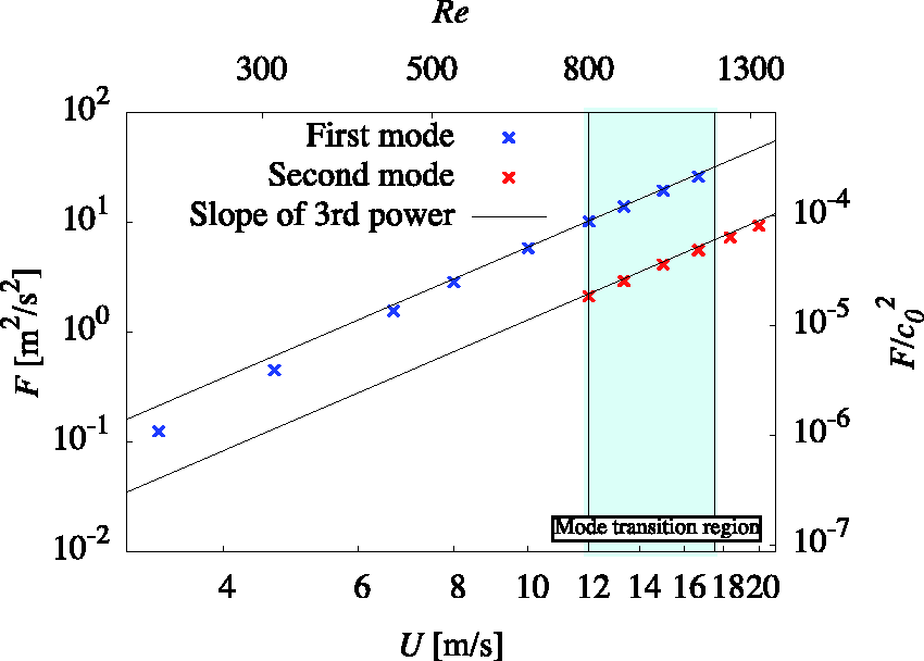
Our ultimate goals are to clarify the underlying generation mechanism of the edge tone by directly evaluating the generation process of aerodynamic sound from the oscillating jet and to comprehensively understand the sounding mechanism of air-jet instruments driven by the edge tone. In this paper, as the first step, we study a 2 D model of the edge tone with the compressible DNS, 26 to check the reliability of the numerical method and to discover new features related to the jet motion and the edge tone generation mechanism. Specifically, we consider a jet with a parabolic inlet profile, because it is more stable than a jet with a top-hat inlet profile.4,23 In particular, we study the following problems. First, we consider the problem of how the intensity of the edge tone changes with the jet velocity for the first and second oscillation modes, namely the power law of the sound intensity, and we explore the mechanism of the dynamical transition observed in the mode transition region. Next, the spatial profiles of the velocity and the velocity variance of the oscillating jet are investigated for each mode over a range of the jet velocity including the mode transition regime. In particular, we introduce a novel measure based on the jet velocity variance profile as a measure of fluctuation strength that scales with jet inlet velocity. We also discuss the difference in the jet motions of the first and second modes.
The organization of this paper is as follows.
In ‘Sounding mechanism of edge tone’ section, we briefly explain the basic properties of the edge tone by using Brown’s equation, 1 We also explain that the edge tone radiated from a dipole-like source follows a 6th-power law, and the power index of the radiation is decreased by one for the 2 D systems, namely a 5th-power law is observed for the 2 D edge tone.2,27
In ‘Model and numerical method’ section, we introduce the 2 D model of the edge tone studied in this paper and explain the numerical method, compressible DNS, 26 together with the numerical set up.
In ‘Numerical results: Dynamical mode transition and sound intensity’ section, we present results of the investigation of jet oscillation modes and their dependence on jet velocity. First, we consider pressure and velocity distributions. Then, we consider the frequency of oscillations, comparing with Brown’s formula. Finally, we consider the dependence of sound intensity on jet velocity.
In ‘Numerical results: Velocity profile and velocity variance of oscillating jet’ section, we consider the change of properties of the jet motion with the jet velocity. First, we investigate the temporal modulation of spatial profiles of velocity and introduce the skewness of the profile to characterize the temporal modulation. Next, we study the velocity variance of the jet fluctuation that is defined as the square of the standard deviation of the temporal fluctuation of velocity and is a function of the coordinate. The amplitude of the velocity variance profile, named the fluctuation strength, is introduced to characterize the strength of the jet fluctuation. In particular, we consider the problem of how the fluctuation strength changes with the jet velocity for the first and second oscillation modes, namely the power law of the fluctuation strength. We also introduce a theoretical model of the jet velocity profile, a skew-Bickley profile model, to support our numerical observations.
The final section is devoted to the summary and discussion.
Sounding mechanism of edge tone
Mode transition of edge tone
In this subsection, we review basic properties of the edge tone. As shown in Figure 1, a jet emitted from a flue collides with an edge and causes vortices. This interaction with the edge produces a feedback toward the flue exit, which influences the jet to oscillate in the vertical direction. This cycle of events is repeated periodically and the jet oscillation is sustained.8–10,13 As a result, the aerodynamic sound, known as the edge tone, is created by the oscillating jet together with the vortices.2,8
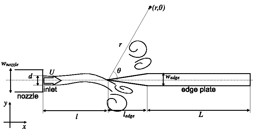
2 D model of the edge tone and schematic picture of the jet. The parameters are taken as l = 5 mm, wedge = 1.2 mm, wnozzle = 2 mm, d = 1 mm, ledge = 3 mm and L = 12 mm. The origin of the polar coordinates (
The relation between the oscillation frequency of the edge tone and the jet injection velocity was experimentally obtained by Brown, i.e., Brown’s equation
1


Mode transition of the edge tone.
Acoustic power radiated from Lighthill’s source
The generation mechanism of aerodynamic sound is formally explained by the Lighthill acoustic analogy. 3 The aerodynamic sound obeys an inhomogeneous wave equation called the Lighthill equation, whose inhomogeneous term plays the role of sound source and is regarded as a quadrupole source. From the properties of the quadrupole source generated by turbulence flow, Lighthill showed that the acoustic energy generated by it is proportional to the 8th power of mean fluid velocity in transonic and subsonic ranges. 3 Since the 8th-power radiation rapidly decreases with decreasing flow velocity, there is a possibility that a power law of different order dominates the sound generation in a range less than subsonic: 4th-power law of monopole-like radiations or 6th-power law of dipole-like radiations. Note that in the case of 2 D systems, the power index of the radiation is usually decreased by one, for example 4th and 6th-power laws change to 3rd and 5th-power laws, respectively (see Table 1).2,27
Power law of sound source.

The pressure distribution of the edge tone is antisymmetric with respect to the edge plate. It is known that the edge tone is radiated from a dipole-like source and obeys a 6th-power law for 3 D systems, that is, a 5th-power law for 2 D systems. 8 From experimental observation for 3 D systems, we expect that it deviates from a 5th-power law in the mode transition region due to the instability of oscillations.
Model and numerical method
Figure 1 shows the 2 D model of the edge tone studied in this paper. The distance between the nozzle and the tip of the edge and the width of the nozzle are respectively taken as l = 5 mm and d = 1 mm. For other dimensions of the model see the figure caption. The ratio
In this paper, we use the compressible DNS for calculating the edge tone, which is the most reliable scheme without any artificial viscosity terms.
26
To handle the boundary condition on the solid surface embedded in a flow field, we adopt the volume penalization (VP) method, which is one of the immersed boundary methods. In the VP method, penalization terms are added to the system of governing equations instead of imposing no-slip boundary conditions at the solid surface:




When the speed of the sound c0 and the mean density ρ0 are given, the mean pressure and temperature are respectively given as 
For spatial derivatives, the sixth-order-accurate compact scheme is used except for the penalization terms for which the fourth-order central scheme is used.26,30 For time evolution, the second-order implicit method is used for the penalization terms, while the second-order Adams-Bashforth method is used for the other terms. To suppress aliasing errors due to nonlinear terms and oscillations due to the penalization terms, the sixth-order compact scheme for filtering is also used at each time step.26,30
We adopt a dimensionless system for numerical calculations, in which the speed of sound c0, the mean density ρ0 and the width of the nozzle d are taken as units of non-dimensionalization. For details, see the previous work.
26
To compare our results with those of the real physical experiments and numerical calculations in the previous works, we fix some of the physical quantities and dimensions of the model, and translate dimensionless quantities to dimensional quantities. In dimensional units, we take
Values of jet velocity U, Reynolds number Re and Mach number M.

Figure 3 shows a mesh of DNS near the operating portion of the edge tone, where the grid interval takes the minimum value, for the case of U = 3.3 m/s with time step
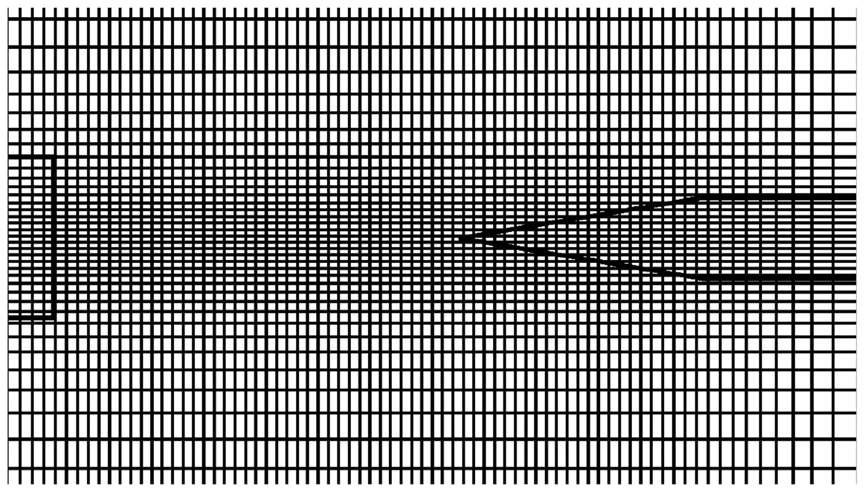
Mesh of DNS: the mesh near the operating portion of the edge tone at U = 3.3 m/s. The lines are drawn every 10 grid intervals.
Figure 4 shows the whole mesh of the computational domain in the dimensionless units, which is divided into four regions, i.e., boundary layer region Rbl, flow region Rf, sound region Rs and buffer region Rbf. The grid interval

The whole mesh of the computational domain in the dimensionless units. Dotted lines indicate the vertical and horizontal center lines.
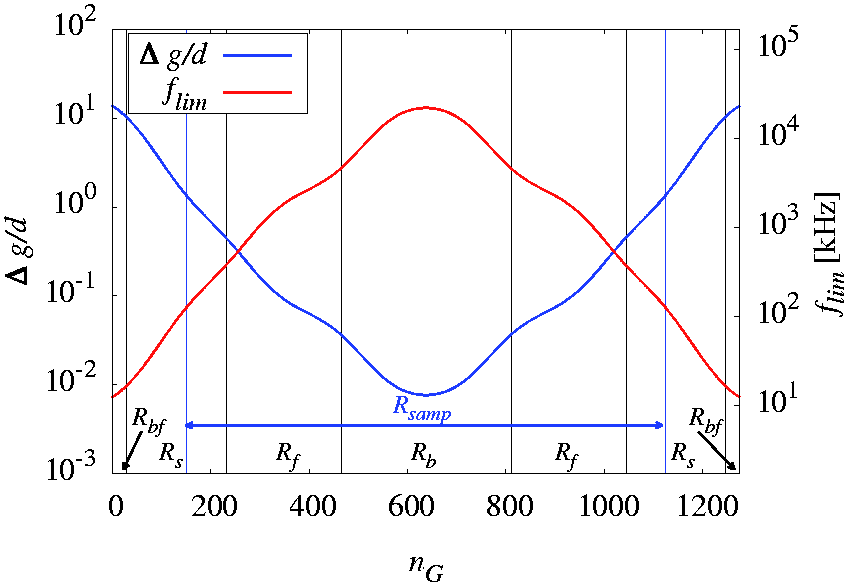
Grid interval
The limit of reproducible sound frequencies flim is determined by the grid width: the formal minimum wavelength
To remove reflection at the outer boundary of the computational domain, the non-reflecting boundary condition introduced by Poinsot and Lele is used.26,31 However, this method does not work completely. To suppress motions in areas near the outer boundary, the computational domain is taken wide enough and the filtering effect is enhanced by taking grid sizes larger.26,30 Thus, the reflection from the outer boundary is almost completely removed.
For calculations, we use the supercomputer, Fujitsu PRIMERGY CX2550/CX2560 M4 (3456 GFLOPS/node). For the cases of U = 3.3 and 20.0 m/s, the calculations of 0.01 sec using 1 node with 36 cores (36 parallel threads) take about 5 and 51 days, respectively. Therefore, a huge calculation time is required to obtain a stationary oscillation in time evolution, which is longer than 0.01 s. It is practically impossible to reproduce the hysteresis of mode transition with sweeping the jet velocity U adiabatically, very slowly. Thus, the jet velocity U is fixed at representative values in the range of 3.3 to 20.0 m/s. In the mode transition region, we observe which mode, the first or second mode, is excited depending on U.
Numerical results: Dynamical mode transition and sound intensity
In this section we present and discuss the results of the numerical study on the dynamical mode transition, frequencies of the edge tone and sound intensity.
Pressure and velocity distributions
First, in this subsection, we consider the properties of pressure and velocity distributions to check the reliability of the numerical scheme and to explore the mechanism of the dynamical transition observed in the mode transition region.
Figure 6(a) and (b) show the distributions of the absolute values of velocity at U = 8.0 and 20.0 m/s, respectively. Figure 7(a) and (b) show the corresponding sound pressure distributions at U = 8.0 and 20.0 m/s, respectively. Note that the sound pressure ps is defined as
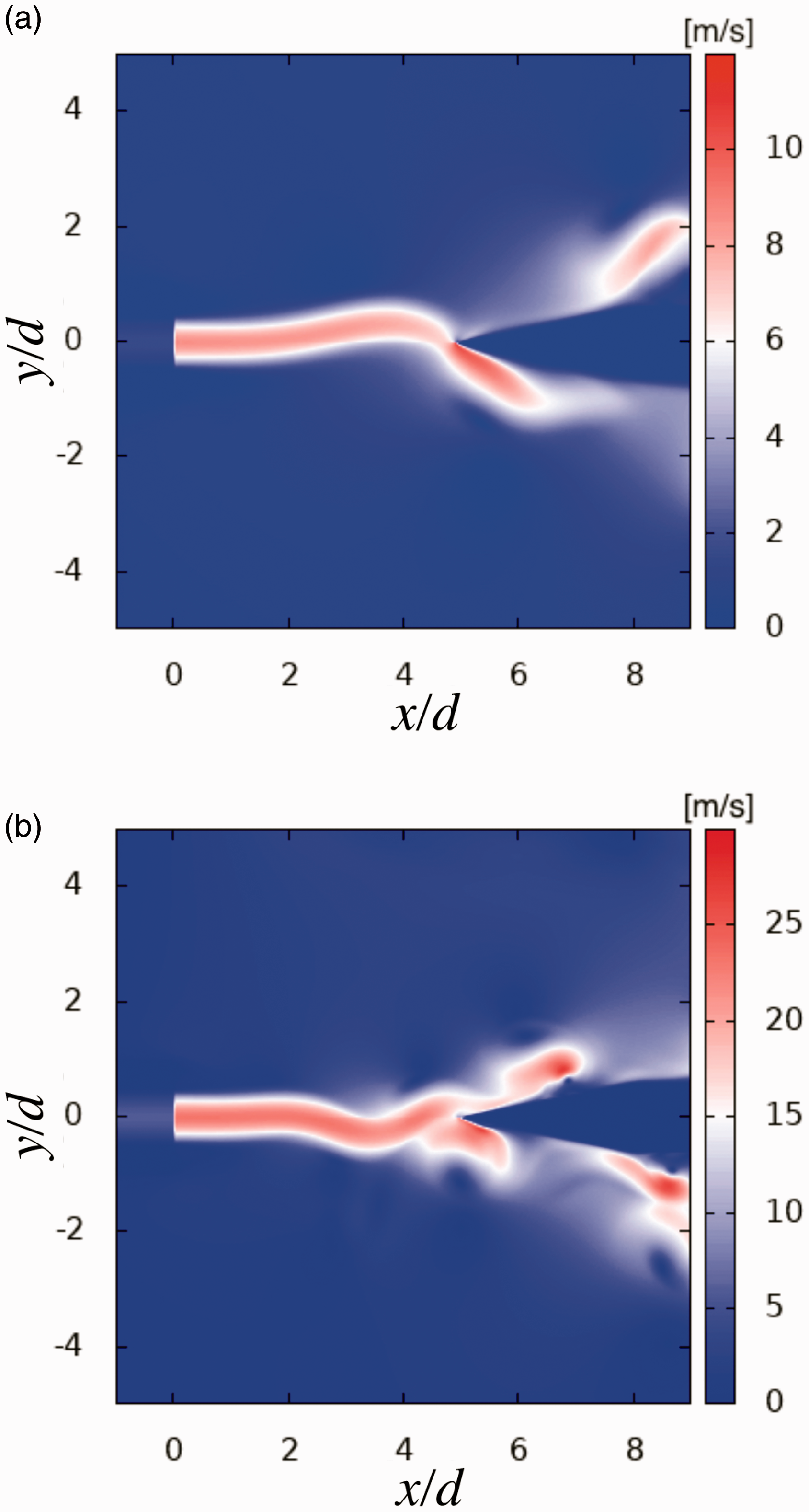
Velocity distributions in the stationary states. The origin of the Cartesian coordinates (x, y) is taken at the center of the inlet. (a) U = 8 m/s. (b) U = 20 m/s.

Sound pressure distributions in the stationary states. (a) U = 8 m/s. (b) U = 20 m/s.
In order to consider the properties of the sound wave, pressure oscillations are observed at the points of
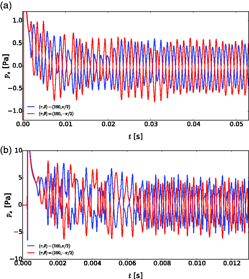
Time evolution of sound pressure ps at the observation points
We show results in the mode transition region, where the first and second modes may appear in the course of time evolution. Namely, transitions between the first and second modes can be observed in time evolution; thus, even if one of the modes is excited, it may change to the other. In our simulations, the jet is sometimes destabilized by vortices, which can trigger a transition.
For example, Figure 9 shows the sound pressure fluctuations at the observation points for U = 16.7 m/s. The transition from the first to second modes is observed in time evolution. Even in this case, the fluctuations of sound pressure at the two observation points are in antiphase to each other. As shown in Figure 10(a) and (b), in the case of U = 16.7 m/s, the first and second hydrodynamic modes of the jet are observed at t = 0.0072 and 0.0142 s, respectively. There are often observed vortices with relatively high velocities near the jet in the mode transition region. They are shed by the interaction of the jet with the edge and drift near the jet. Such strong vortices are often observed in experiments of the edge tone and air-jet instruments.23, 32 Figure 11(a) and (b) show sound pressure radiations of the first mode at t = 0.0072 s and the second mode at t = 0.0142 s in the case of U = 16.7 m/s, respectively. Like those in Figure 7, the sound pressure distribution seems to be antisymmetric with respect to the horizontal line. In this sense, even in the mode transition region, the oscillating jet behaves as a dipole-like source.

Time evolution of sound pressure ps at the observation points for U = 16.7 m/s.
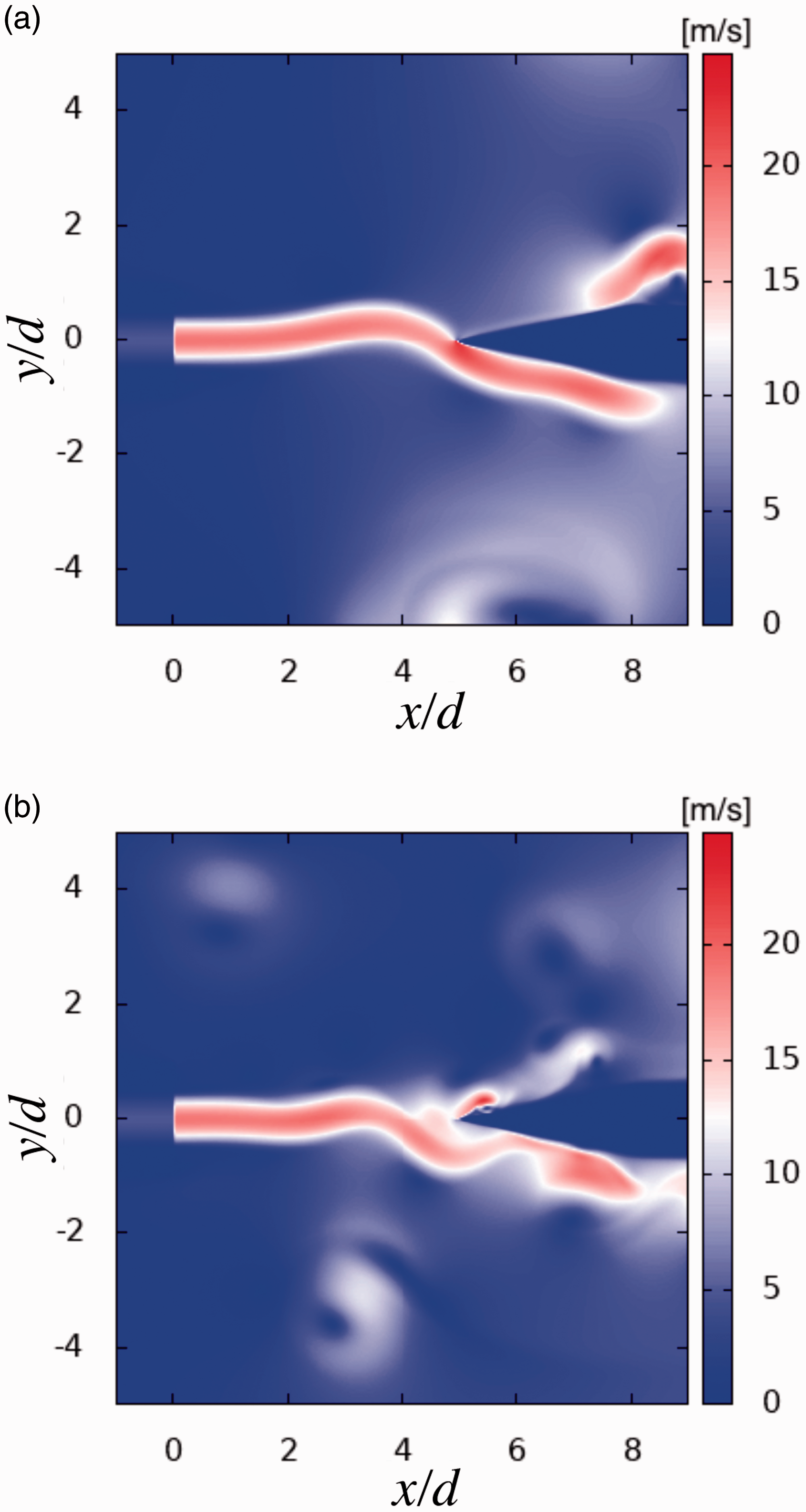
Velocity distributions in the stationary states at U = 16.7 m/s. (a) The first mode at t = 0.0072 s. (b) The second mode at t = 0.00142 s.
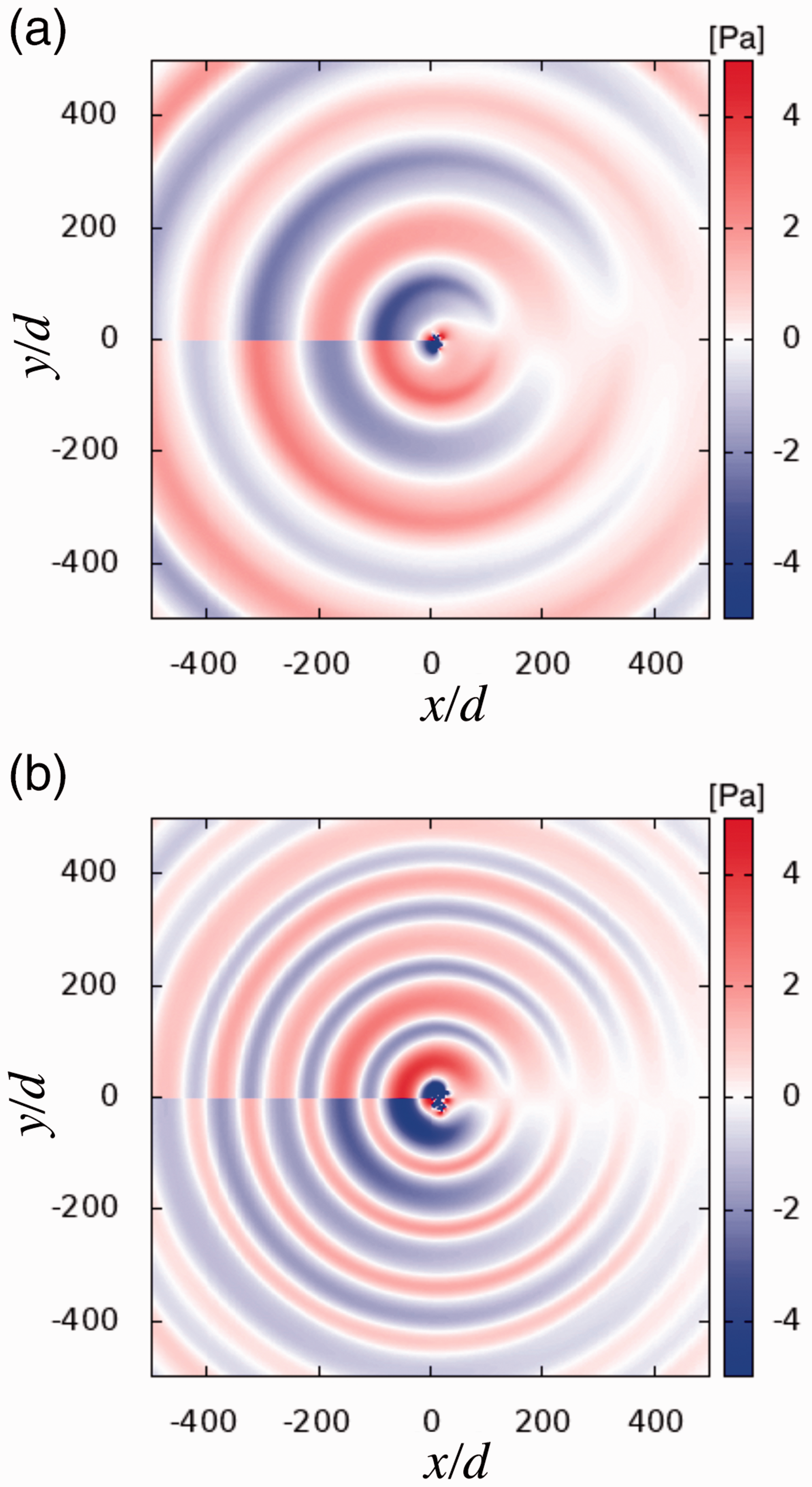
Sound pressure distributions in the stationary states at U = 16.7 m/s. (a) The first mode at t = 0.0072 s, (b) The second mode at t = 0.00142 s.
Let us consider the mechanism of the mode transition. For the case of U = 16.7 m/s, the pressure oscillations are destabilized in the time interval (
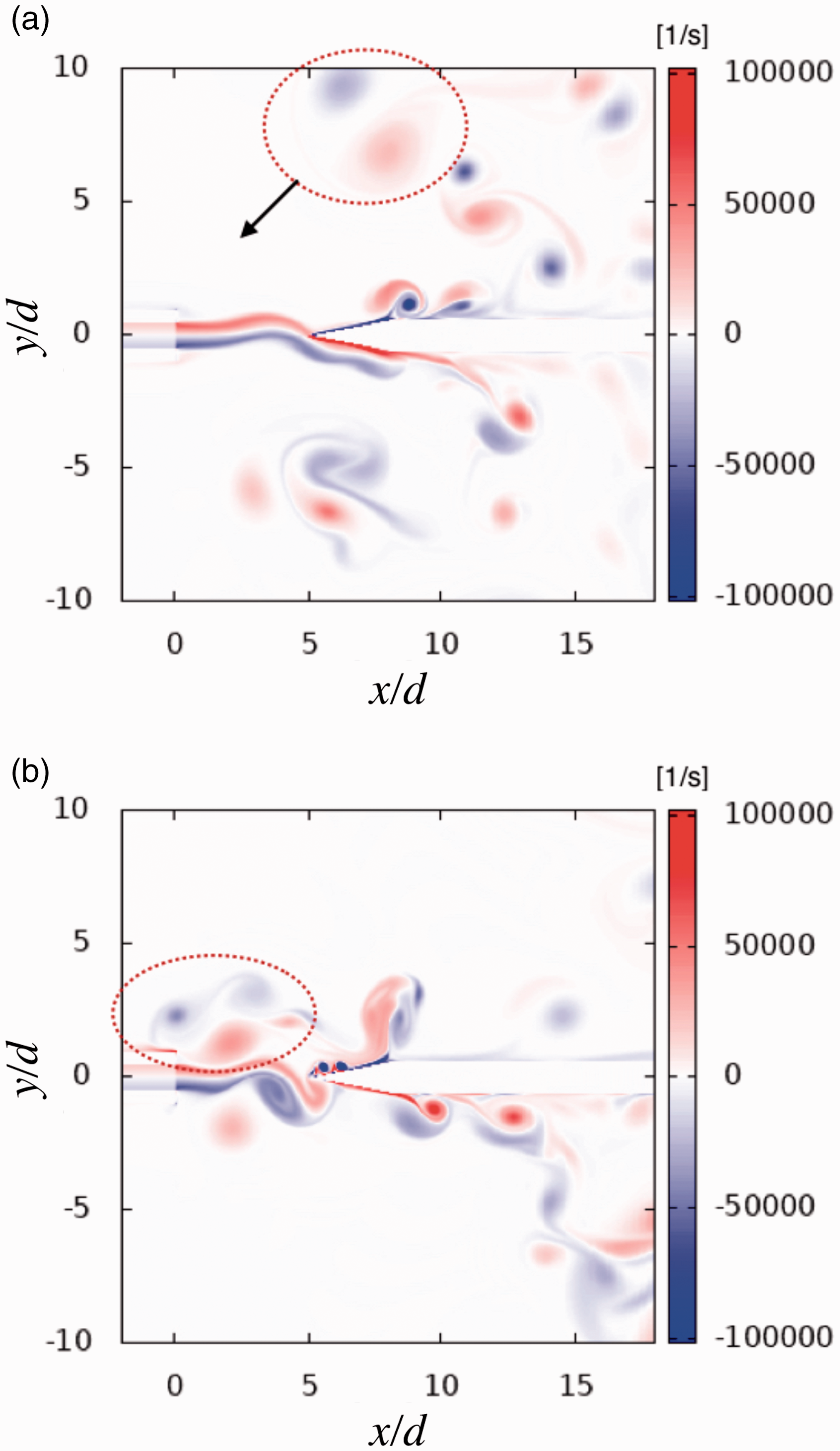
Vorticity distributions at U = 16.7 m/s. (a) t = 0.0072 s. (b) t = 0.011 s.
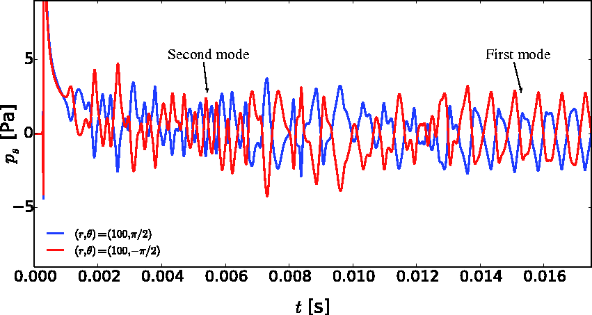
Time evolution of sound pressure ps at the observation points for U = 15.0 m/s.
Disturbance due to the approach of vortices is expected in the whole range of U, though the probability and impact may depend on the value of U. When U is out of the mode transition region, the probability of the disturbance seems to become low and the jet motion should return to the original mode in a recovery process, even if disturbed by vortices. Actually, at U = 6.7 and 10.0 m/s in the first mode range, the jet motions are disturbed by vortices, but they always return to oscillations of the first mode. For the case of U = 10.0 m/s, see Figure 20(a).
Let us comment on similarities and differences compared with other reports of mode transitions. Paál and Vaik found with an incompressible fluid simulation of a two dimensional model that dynamical transitions are often observed at low Reynolds numbers and a superposition of several modes occurs at high Reynolds numbers for a top-hat inlet profile,
21
while a dynamical transition was not observed and each mode was rather isolated even in mode transition regions for a parabolic inlet profile.8,23 They mainly treated the case of
Sound frequency compared with Brown’s equation
For comparison with Brown’s equation (1), we calculate the frequency of the pressure oscillation of the edge tone at the observation points. The calculation times of edge tones with DNS are not long enough to attain acceptable resolutions in frequency by FFT. Therefore, we measure the mean frequency of oscillation as follows. If
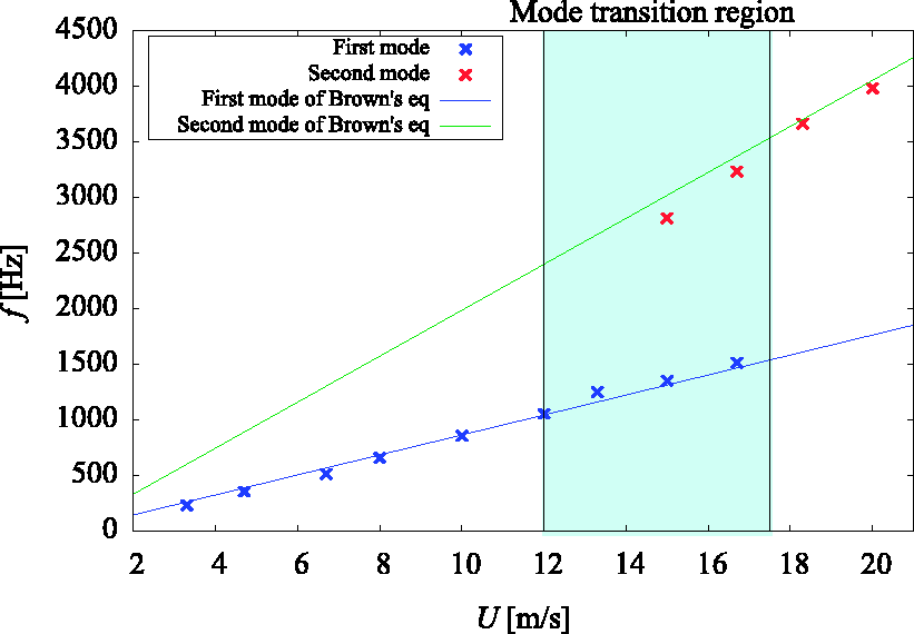
Sound frequencies f obtained from the results of DNS vs. Brown’s equation (1): the blue and red points are frequencies of the first and second modes, respectively.
In Figure 15, the Strouhal number
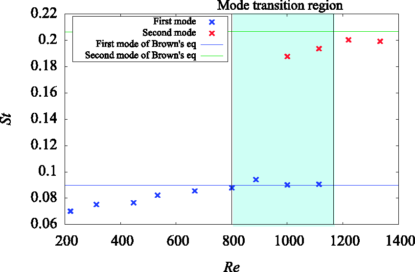
Strouhal number St as a function of Reynolds number Re.
Sound intensity
In this subsection, we consider the change of sound intensity I with the jet velocity U. The sound intensity I is defined as

Figure 16 shows the radiation pattern, the sound pressure amplitude pa at
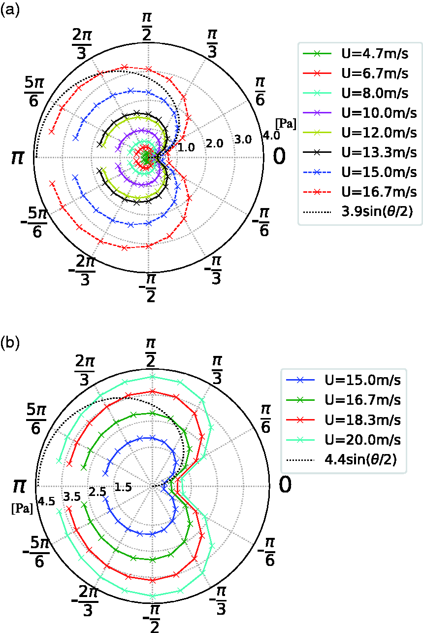
Changes of the sound pressure amplitude at
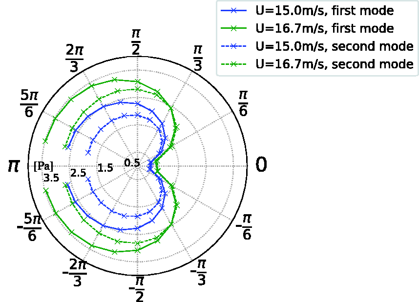
Changes of the sound pressure amplitude at
The shape of the radiation pattern of the first mode shown in Figure 16(a) seems to be close to a cardioid. Ffowcs Williams and Hall discussed the case that a solid half plane is embedded in a turbulence flow, which can be applied to a two dimensional situation because they supposed uniformity in the direction of z. They showed that the sound intensity, which is proportional to the square of the sound pressure, changes as a cardioid as a function of the angle θ and obeys the 5th-power law U.5,16 Even though an additional finite length edge plate exists in our case, their formula seems to be applicable to our results. The shape of the sound pressure radiation pattern of the first mode is similar to that of the square root of the cardioid function,
Figure 18 shows the changes of the sound intensity of the first and second modes as functions of the jet velocity U, where each sound intensity is calculated from the maximum value of the sound pressure amplitude pa. The black lines are the slopes of 5th power. For both first and second modes, the sound intensity follows a 5th-power law as expected for dipole-like radiations. However, the intensity of the second mode is less than that of the first mode. The sound intensity of the first mode is 2.36 times larger than that of the second mode. Note that the sound intensities observed in experiments each obey a 6th-power law, but different modes have different intensity values.8–10 Therefore, our numerical results correspond to a 2 D analog of the dipole-like radiation observed for the edge tone. Furthermore, in the mode transition region, the intensity of the first mode is suppressed and deviates from the upper black line while that of the second mode is also suppressed slightly. In addition, in a low velocity range, e.g., U = 3.3 m/s, the intensity drops off and deviates from the 5th-power law.
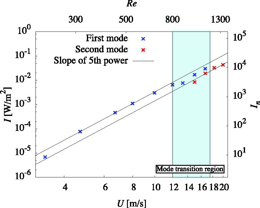
Changes of the sound intensity I for the first and second modes with the jet velocity U. The dimensionless sound intensity In is defined as
Numerical results: Velocity profile and velocity variance of oscillating jet
In this section, we study the properties of the jet motion in detail. Specifically, we explore how the transverse spatial profiles of jet motion and jet fluctuation change with increasing jet velocity. We also discuss the difference in the jet motions of the first and second modes.
Jet motion and velocity profile
In this subsection, we investigate transverse profiles of the oscillating jet. To do this, we fix the observation line parallel to the vertical axis at a distance of 3.0 mm from the nozzle (
Figure 19 shows snapshots of normalized velocity profiles

Changes of the normalized velocity profile
To quantify the degree of asymmetricity of velocity profiles, we calculate the skewness sU of the profile. Details are shown in the Appendix 1. Table 3 shows the skewness sU of velocity profiles in Figure 19. From the definition given by equation (15), the skewness sU is related with the difference in gradient between the right and left slopes of the normalized velocity profile q/U. At the center positions,
Skewness sU defined by equation (15) for velocity profiles in Figure 19.

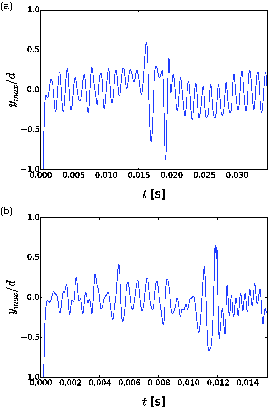
Oscillations of the maximum point ymax of the velocity profile at
Next, we consider the amplitude of the jet oscillation in the transverse y direction. We let ymax represent the value of y at which the velocity profile has maximum value at time t. This maximum point oscillates almost periodically when the system is in stationary mode oscillation. We define the amplitude of jet oscillation in the y-direction as the amplitude of oscillation of the maximum point ymax, and denote it by aj. Figure 20(a) and (b) show oscillations of ymax at U = 10.0 and 16.7 m/s, respectively. Figure 21 shows the changes of the amplitude of the jet oscillation aJ with U for the first and second modes. The oscillations at U = 10.0 and 16.7 m/s are relatively unstable and have a low-frequency drift even in a duration of a single mode due to the disturbance of vortices compared with more stable cases (see the error bars in Figure 21). Indeed, the sound pressure oscillations at U = 8 and 20 in Figure 8 are much more stable than that at U = 16.7 in Figure 9.
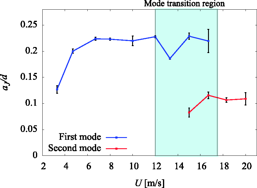
Changes of the amplitude of the jet oscillation aJ at
At U = 16.7 m/s in Figure 20(b), a stable oscillation of the first mode is observed in the range
As shown in Figure 21, the amplitude of the first mode increases until U = 6.7 m/s and slightly decreases in the range
Fluctuation of velocity distributions of the jet
To study the properties of the velocity variation in the transverse vertical line, we introduce the velocity variance profile defined by


When the coordinate y is fixed,
Figure 22(a) and (b) show the normalized velocity variance profile
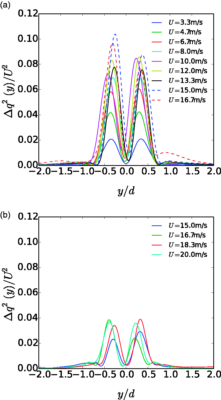
Normalized velocity variance profile

Time evolution of q(y, t) at
For the first mode, the two peaks of
The two-peak variance profile of 
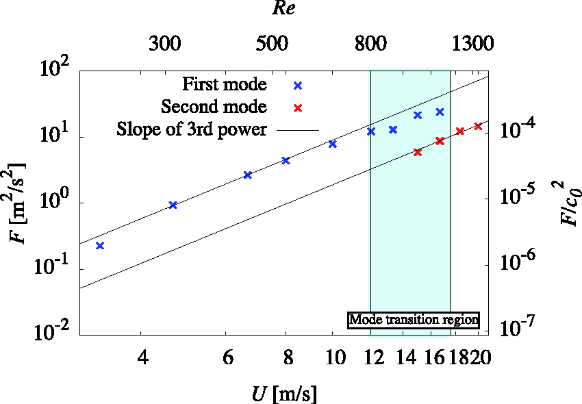
Changes of the fluctuation strength F for the first and second modes with the jet velocity U. The black lines have slopes corresponding to the 3rd-power law.
Theoretical model for velocity profile
In this subsection we briefly discuss theoretical aspects of the power law behavior. First, we point out that the 3rd-power law behavior of the fluctuation strength F (that is, the amplitude of the velocity variance profile) is not expected from the common lowest-order model of the velocity profile. Then we present a modified model that is consistent with the above observations of both the velocity profile q(y, t) and the velocity variance profile
The first order approximation of the velocity profile of a static jet is given by a squared hyperbolic-secant function called the Bickley profile.
29
As the lowest order approximation, the velocity profile of the oscillating jet can be represented by
34


To support the hypothesis, we introduce a modified model of velocity profile, which reproduces the 3rd-power law under the condition that the skewness increases with the jet velocity and the amplitude of jet oscillation is saturated. The detail requirements for the model are as follows. When U is fixed, the velocity profile is periodically deformed, but the volume flow is held constant. At the leftmost and rightmost positions,
We rely on the idea of the skew-normal distribution that generalizes the normal distribution to allow for non-zero skewness by using the error function, the antiderivative of the Gaussian function.
35
Since 

To adjust the model to the numerical situation, the parameters are set as follows. The width of the velocity profile wy is set as
Figure 25(a) shows the changes of the amplitude of the jet oscillation aJ with increasing U for the first and second modes. The amplitude of the first mode increases in the range U < 10.5 m/s, but it slightly decreases for U > 10.5 m/s. The normalized amplitude
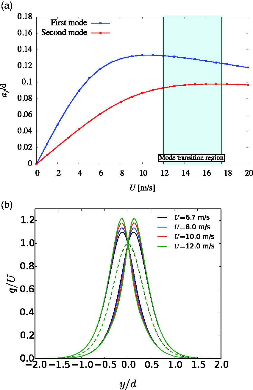
Properties of the skew-Bickley profile model. (a) Changes of the amplitude of jet oscillation aJ with U for the first and second modes. (b) Changes of the normalized velocity profile
Skewness sU of velocity profiles at the leftmost positions in Figure 25(b).

Figure 26(a) and (b) show the normalized velocity variance profiles
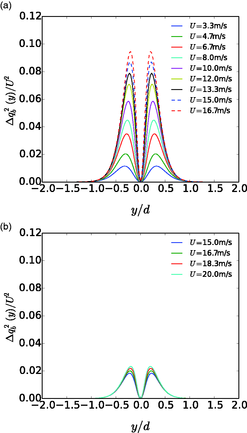
Normalized velocity variance profile
Changes of the fluctuation strength F for the first and second modes with U for the skew-Bickley profile model. The black lines have slopes corresponding to the 3rd-power law.
The above analysis of the skew-Bickley profile model indicates that the increase of
Summary and discussion
In this paper, we calculated motions of two-dimensional compressible fluid generating edge tones with a high-precision integration scheme, compressible DNS, when a jet with a parabolic inlet profile is injected. First, a transition of the hydrodynamic mode is observed with increasing jet velocity, namely the transition from the first mode to second mode, which induces the transition of the acoustic mode of the edge tone. The frequencies of the acoustic oscillations agree well with Brown’s equation for both first and second modes. 1 When the jet velocity takes a value in the mode transition region, changes of oscillations from the first mode to the second mode and vice versa are observed in time evolution. Namely, the system in the mode transition region can be regarded as a bistable system with two attractors from the view point of nonlinear dynamics. 28 Thus, even if the jet stationarily oscillates in one of the modes, a sudden disturbance due to the approach of vortices would induce a transition to the other mode. This mechanism is different from that observed for a top-hat inlet profile in the previous works.21,23
The acoustic pressure distribution observed numerically is antisymmetric with respect to the horizontal axis as observed in experiments. 8 This means that the edge tone is radiated from a dipole-like source. For both first and second modes, the sound intensity well follows a 5th-power law, which corresponds to a 6th-power law in three dimensional systems; 8 thus, this is another evidence that the edge tone is radiated from a dipole-like source. It was observed that the intensity of the second mode is less than that of the first mode. Furthermore, for the first mode, the intensity is suppressed and deviates from the 5th-power law at both ends of its oscillation range. The second mode shows the same tendency at the lower end of its oscillation range. Similar deviations from the 6th-power law at the ends of the oscillating range of each mode are observed experimentally. 8 From the above results, it can be seen that our numerical calculations well reproduce the properties of the edge tone in detail and it is safe to say that the compressible DNS is a reliable tool for analyzing the sounding mechanism of the edge tone.
To consider the change of the fluctuation strength of the jet motion with the inlet jet velocity, we studied the spatial profiles of the velocity q(y, t) and the velocity variance of the oscillating jet
The change of the fluctuation strength F with U shows the same tendency as that of the sound intensity. This indicates a physical correspondence between the velocity fluctuation of the oscillating jet, the sound source, and the radiated sound. The results of the simulation reported in this paper motivate us to calculate the Lighthill’s acoustic source terms, i.e., the first and second terms, in an accurate manner and to clarify the relation of the source terms with the radiated sound based on the Lighthill acoustic analogy together with the Curle analogy or the Ffowcs Williams-Hawkings analogy.3,14,15 Furthermore, the demonstrated reliability of the simulation method is encouraging for other detailed numerical studies of 2 D models of air-jet instruments.
Footnotes
Acknowledgements
The authors are very grateful to Dr. P. Davis (Telecognix Co.) for useful discussions and proofreading our English writing.
Declaration of conflicting interests
The author(s) declared no potential conflicts of interest with respect to the research, authorship, and/or publication of this article.
Funding
The author(s) disclosed receipt of the following financial support for the research, authorship, and/or publication of this article: The present work was supported by Grant-in-Aid for Scientific Research (C) Nos. 16K05477 and 19K03655 from the Japan Society for the Promotion of Science (JSPS), “Joint Usage/Research Center for Interdisciplinary Large-Scale Information Infrastructures” and “High Performance Computing Infrastructure” in Japan (Project IDs: jh190010-MDH and jh200001-MDH), and Kawai Foundation for Sound Technology & Music. Part of the work was carried out under the Collaborative Research Project of the Institute of Fluid Science, Tohoku University.

Appendix 1. Definition of skewness.
The skewness of velocity profile sU is defined by