A bionic noise reduction strategy on the trailing edge of NACA0018 based on the central composite design method

Abstract

New innovative approaches to reduce noise are of great significance in engineering. Taking the typical NACA0018 airfoil as the study target, the serrated treatment of the trailing edge is carried out with the bionic noise reduction technology. To boost the design efficiency and clarify the distributing laws between the design parameters and the noise performances, a special investigation about optimizing the NACA0018 airfoil’s serrated trailing edge is implemented here. Firstly, a united parametric approach to represent various design schemes is proposed. Then, with the integration of the Computational Fluid Dynamics/Computational Acoustics analysis, Central Composite Design, and the Respond Surface Method, a bionic noise reduction strategy is established. The findings can be gotten as: taking into account the existence of the casing or wall near the span-end of the airfoil, the newly defined install location adjustment factor has an influence on the reduction noise, and the install location adjustment factor mainly affects the near-wall flow field of the serrated trailing edge; the optimal design scheme is obtained successfully, which can reduce the overall sound pressure level by about 2 dB in relative to the target; through the mechanism analysis of noise reduction, it can be found that the serrated trailing edge can suppress the development of the laminar separation bubbles, so the noise is reduced.

Keywords

Bionic noise reduction serrated trailing edge install location adjustment factor new innovative approach central composite design

Introduction

The noise problem is causing much more attention in various modern industries, as a result, noise reduction technology has become a hot topic, especially in the aviation area.^1–3 The noise control technology affects not only the environmental issues, but also the product competitiveness. For the aircraft, the turbulent broadband noise control is still a difficult problem, mainly including the airfoil’s trailing edge of self-noise.⁴

To reduce the trailing edge noise, many noise reduction technologies were proposed, for instance, the porous media,⁵ the trailing edge blowing,⁶ the bionic noise reduction,⁷ etc. In recent years, bionic noise reduction technology has been concerned and adopted. By learning the phenomenon of the owl’s quiet flying, the trailing edge serration based on the owl’s wings has been studied. Howe⁸ firstly proposed the model of the serrated trailing edge. After that, several numerical, experimental, and theoretical studies^9–13 about the airfoil with serrated trailing edges have proved the serration’s noise reduction ability. Lau and Xun¹⁴ compared four models (triangle, serration, sinusoid, and slot), and it was found out that the serration had the best noise reduction ability.

Continually, the effects of the serration sizes on the noise have been extensively studied. Gruber et al.¹⁵ investigated the effects of the serrate tip-to-root distance H and wavelength λ on noise reduction with NACA65 airfoil. It was found that the larger the ratio of H to λ was the much more obvious the noise reduction effect would be. However, Moreau and Doolan¹⁶ came to a completely contrary and different conclusion that the noise reduction effect would decrease with the improvement of the ratio of H to λ. Additionally, hypotheses and explanations for the serration noise reduction mechanism were not so united. Lyu et al.¹⁷ proposed that the noise reduction may be caused by the phase difference among the scattered pressure waves near the trailing edge. Chong et al.¹⁸ assumed that edge vortices appeared on a serrated trailing edge surface, which suppressed the separation vortices at the trailing edge.

Though numerous studies on the serrated trailing edge have been implemented, the research is still insufficient. First of all, in terms of the contradiction between Gruber and Moreau, the effects of the serration sizes need to be further clarified. Additionally, the previous research on the trailing edge’s serrated treatment mainly focused on two parameters, namely the serrate tip-to-root distance H and the wavelength λ (or the serrated number n), which can determine the serration shape. However, as presented in the red circle of Figure 1(a), the airfoil is installed on the casing, and in Figure 1(b), it can be found that the root shape of the airfoil on the casing would play an extremely important role in determining the flow stability. As a result, an install location adjustment factor φ which adjusts the install position of the serration near the casing was added in this study.

Figure 1.

Significance of the install location adjustment factor: (a) airplane model and (b) pressure distribution with different install location adjustment factors.

With the whole consideration of the newly proposed install location adjustment variable in this study and the previous settled variables, the corresponding composite effects would be herein investigated and explored. Taking the typical NACA0018 airfoil as the study target, a bionic noise reduction strategy established on a new parametric design approach, and Central Composite Design (CCD) was proposed to find out the optimal structures. Most importantly, the effects of the serration install location on the noise reduction were investigated and clarified during the optimization process. The study was organized as follows: the second section gave the specific details about the numerical approach and its validation; the third section presented the newly developed parametric approach; the fourth section introduced the bionic noise reduction strategy and showed its application; the fifth section illustrated the effectiveness of the optimal result by making a mechanism comparison with the reference model; the final section provided the conclusions.

Validation of the numerical methodology

The target model

As a typical airfoil, NACA0018 was widely taken as the research object for the airfoil noise reduction by many scholars,¹⁹,²⁰ which was still taken as the target model in this study. Fujisawa et al.²¹ has measured the noise field around the NACA0018 airfoil with zero angle of attack, which would supply abundant validating data for the numerical methodology of the study. The NACA0018 airfoil’s 3D model was presented in Figure 2(a), while the calculation domain was shown in Figure 2(b).

Figure 2.

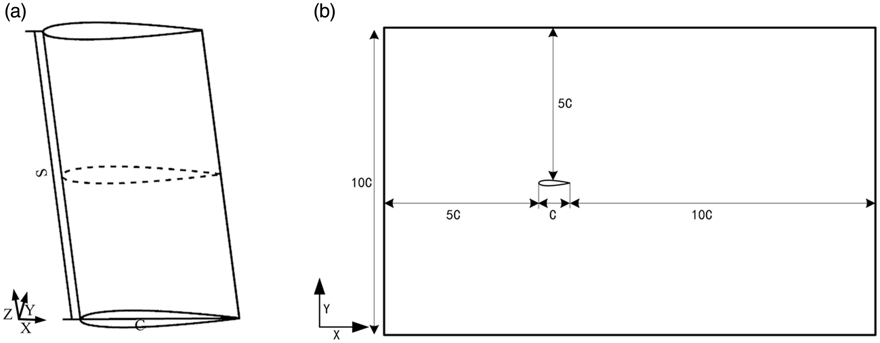
Study object: (a) NACA0018 airfoil, (b) calculation domain.

According to the calculation domain²² and the experimental condition,²¹ the airfoil chord length and span length for the 3D model were set as C = 100 mm and S = 200 mm, respectively. Moreover, the Reynolds number was Re = 1.6 × 10⁵, whose corresponding flow speed was U_o = 24 m/s via the conversion formula.

Settings of the numerical approach

The solving process was performed in the ANSYS-FLUENT solver.²³ The boundary conditions for calculation were velocity inlet, pressure outlet, and non-slip wall. The medium could be considered as the incompressible flow with a low Mach number of 0.07. A finite volume method with structured meshes and an incompressible large-eddy simulation were employed to solve the time-dependent turbulent flow. The wall-adapting local eddy-viscosity (WALE) model was used to compute the subgrid-scale eddy viscosity, which can correctly handle the laminar zones in the domain. The spatially filtered Navier-Stokes equations were solved by the SIMPLEC algorithm. When the convergence is limited by the pressure-velocity coupling, the SIMPLEC algorithm makes convergence more quickly. The convection and diffusion terms were discretized by the second-order bounded central differencing scheme. Considering the calculating accuracy, the second-order implicit scheme was used for time marching. The sound field results were calculated by the Ffowcs Williams-Hawkings (FW-H) equation.

The sampling time was set to be 0.1 s, whose frequency spacing was 10 Hz. Since the maximum frequency was 10 kHz, the time step can be settled down according to the Nyquist sampling theorem

Δ t = \frac{1}{2 f_{\max}} = 5 \times 10^{- 5} s

(1)

Large Eddy simulation

The filtering of the continuity equation and momentum transport equation were introduced in large Eddy simulation (LES). The filtering operation can be expressed as²⁴

\bar{F} (x) = \int_{D} G (x - z, Δ) F (z) d z

(2)

where

G

is the Gaussian filter;

F

is the variable;

Δ

is the subgrid characteristic length scale;

D

is the domain of concern. After filtering the equation, the LES continuity and transport equations in transient stare can be settled down as

\frac{\partial \bar{u_{i}}}{\partial x_{i}} = 0

(3)

\frac{\partial \bar{u_{i}}}{\partial t} + \frac{\partial}{\partial x_{j}} (\bar{u_{i}} \bar{u_{j}}) = - \frac{1}{ρ} \frac{\partial \bar{P}}{\partial x_{i}} + υ \frac{\partial}{\partial x_{j}} (\frac{\bar{u_{j}}}{\partial x_{j}}) + \frac{\partial (\bar{τ_{i j}})}{\partial x_{j}}

(4)

where

\bar{u_{i}}

and

\bar{u_{j}}

are the filtered velocity component;

υ

is the kinematic viscosity;

ρ

is the fluid density;

\bar{P}

is the grid-scale static pressure;

\bar{τ_{i j}} = (\bar{u_{i}} \bar{u_{j}} - \bar{u_{i} u_{j}})

is the subgrid-scale stress tensor. Model the subgrid-scale tensor based on an eddy-viscosity assumption:

\bar{τ_{i j}} = 2 υ_{t} \bar{S_{i j}} - \frac{1}{3} δ_{i j} \bar{τ_{k k}}

(5)

where

υ_{t}

is the eddy-viscosity;

δ_{i j}

is the strain rate tensor at the solution scale;

\bar{S_{i j}}

is the deformation tensor of the resolved field

\bar{S_{i j}} = \frac{1}{2} (\frac{\partial \bar{u_{i}}}{\partial x_{j}} + \frac{\partial \bar{u_{j}}}{\partial x_{i}})

(6)

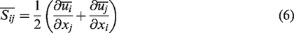
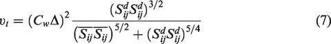
The system of equations (3) to (5) is solved by the WALE model that is determined as

υ_{t} = {(C_{w} Δ)}^{2} \frac{{(S_{i j}^{d} S_{i j}^{d})}^{3 / 2}}{{(\bar{S_{i j}} \bar{S_{i j}})}^{5 / 2} + {(S_{i j}^{d} S_{i j}^{d})}^{5 / 4}}

(7)

where

S_{i j}^{d} = \frac{1}{2} ({\bar{g}}_{i j}^{2} + {\bar{g}}_{j i}^{2}) - \frac{1}{3} δ_{i j} {\bar{g}}_{k k}^{2}

;

C_{w}

is a constant.

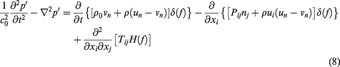
FFOWCS Williams–Hawkings equation

To solve the problem of fluid acoustics, Ffowcs Williams and Hawkings proposed the FW-H equation²⁵

\frac{1}{c_{0}^{2}} \frac{\partial^{2} p^{'}}{\partial t^{2}} - \nabla^{2} p^{'} = \frac{\partial}{\partial t} {[ρ_{0} v_{n} + ρ (u_{n} - v_{n})] δ (f)} - \frac{\partial}{\partial x_{i}} {[P_{i j} n_{j} + ρ u_{i} (u_{n} - v_{n})] δ (f)} + \frac{\partial^{2}}{\partial x_{i} \partial x_{j}} [T_{i j} H (f)]

(8)

and

T_{i j} = ρ u_{i} u_{j} + P_{i j} - c^{2} (ρ - ρ_{0}) δ_{i j}

(9)

where

p^{'} = (p - p_{0})

is the variable quantity of the far-field sound pressure;

ρ_{0}

is the undisturbed fluid density;

ρ

is the disturbed fluid density;

c_{0}

is the far-field sound velocity;

u_{i}

is the component of the fluid tangential velocity in the direction

x_{i}

;

u_{n}

is the outward normal from

f

of fluid velocity;

v_{n}

is the outward normal from

f

of solid boundary velocity;

δ (f)

is the Dirac delta function;

H (f)

is the Heaviside function;

f

is the solid boundary function;

T_{i j}

is the Lighthill stress tensor;

P_{i j}

is the compressible stress tensor.

The complete solution includes twice surface integrations and once volume integration. The monopole, dipole, and partial quadrupole sources are obtained by the surface integration, while the spatial quadrupole sources outside the surface are calculated by the volume integration.

The validating results

The mesh quality affects the accuracy of the numerical calculation results, so the grid number needs to be determined. Three kinds of grids (6 million, 8 million, and 10 million) were selected to be investigated. The partial enlarge drawing for these grids were shown in Figure 3.

Figure 3.

Local mesh on the target model: (a) 6 million, (b) 8 million, (c) 10 million.

For the FW-H equation, it’s more suitable for far sound field calculation. Considering the airfoil size and the characteristic of the FW-H equation, the 36 sound field points were evenly distributed on the circle. As presented in Figure 4, the center was the airfoil’s centroid and the radius of the circle was 1.0 m.

Figure 4.

Sound field point distribution.

Finally, three sets of structured mesh were calculated by the numerical methodology in Part 2.1 and the ranges of frequencies were the same as the experiment (0 Hz–10 kHz). The overall sound pressure level (OASPL) is determined as in equation (10)

OASPL = 10 \times \lg (\frac{\sum_{i = 1}^{n} p_{i}^{2}}{p_{ref}^{2}})

(10)

where p_ref is the reference pressure, whose value is 2 × 10⁻⁵Pa; p_i is the effective sound pressure at different frequencies.

The numerical results of different grids were shown in Figure 5, and it can be seen that the overall results of 8 and 10 million are more similar. To further test the gird, the numerical results of the different grids would be compared with the experimental results.²¹

Figure 5.

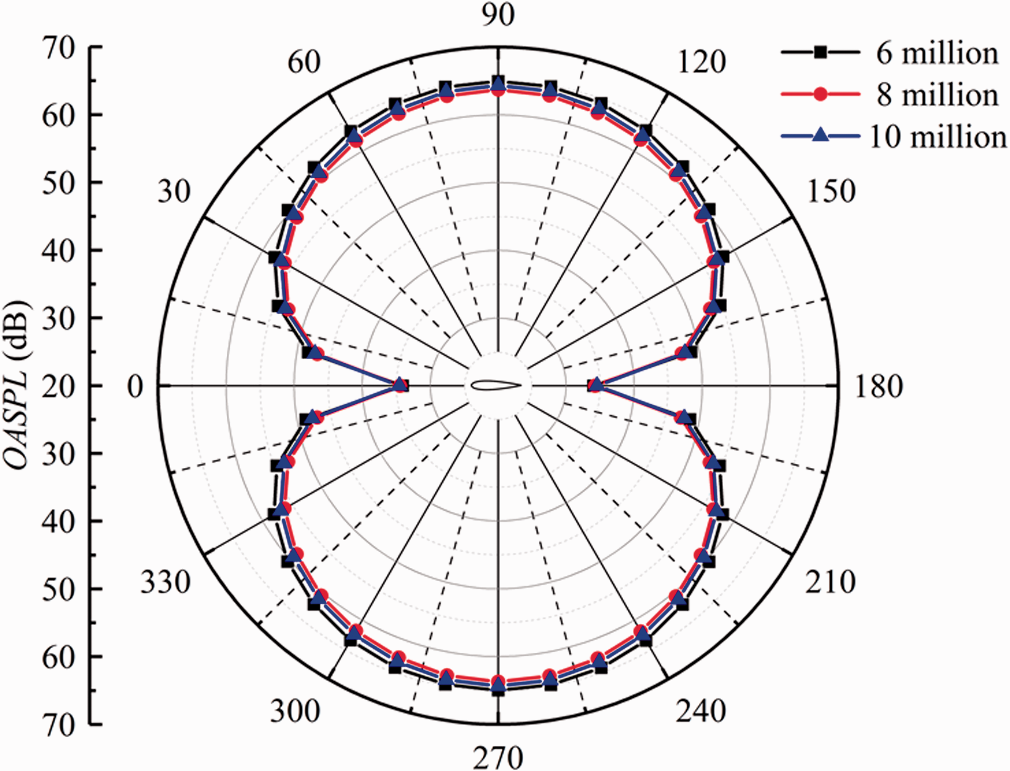
Mesh independence test.

For the Fujisawa’s experiment,²¹ the testing points were different from the selected monitoring points, which were presented in Figure 6. In the figure, these sound field points were located in the place of 95 mm away from the upper and lower airfoil’s centroid. According to the experimental settings, the same points were calculated to compare with experimental data.

Figure 6.

Experimental sound measurement.²¹

Table 1 showed the comparison of the different grids between the experimental result and the numerical result. From the table, it can be known that the errors of the 8 and 10 million were both controlled to be less than 1.5%, which can satisfy the accuracy standard.²⁶ Besides, the numerical result of the 8 million was closer to the experimental value. With the considering of the calculating time and the errors, the grid number in this study was finally chosen to be 8 million.

Table 1.

Comparison of the OASPL.

	Experimental value (dB)	6 million numerical value (dB)	Error (%)	8 million numerical value (dB)	Error (%)	10 million numerical value (dB)	Error (%)
Upper point	87.8033	89.3020	1.71	88.8914	1.24	89.0713	1.44
Lower point	87.7305	89.2875	1.77	88.8787	1.31	89.0416	1. 49

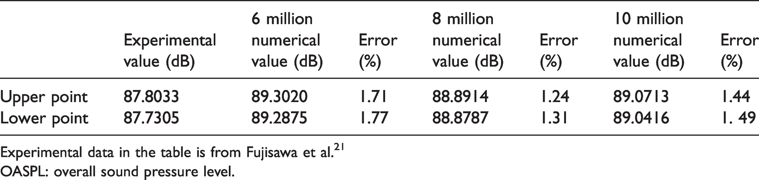
Experimental data in the table is from Fujisawa et al.²¹

OASPL: overall sound pressure level.

To further validate the meshing size and numerical method, the dimensionless wall-cell sizes Y+ along the airfoil and the sound pressure level spectrum were given in Figure 7. For the Y+ value, it should be below 1 for the LES,²⁷ so it can be seen that the selected grid can meet the calculation needs of the Y+ value from Figure 7(a). In Figure 7(b), the gross trend was the same and the peak value appeared at the same frequency location. Overall, through the comparative analysis, the meshing size and the numerical methodology were validated and can be used to predict the NACA0018 airfoil’s noise.

Figure 7.

Comparison of the spectrum. Experimental data in the plots is from Fujisawa.²¹

The parametric approach

Presented in Figure 8, the parameterization for the serration on the airfoil’s trailing edge was mainly consisted of two parts, namely, configuration for the serration shape and adjustment for the serration’s install location. First of all, in terms of the serration shape, it can be settled down with the most commonly used variable of tip-to-root distance H and serrated number n. Then, different from the previous studies, the install location adjustment factor φ which adjusts the install position of the serration was herein defined and proposed. As enlarged in the red box, the install location adjustment factor can adjust the install position of the serration near the casing. After the serration shape was configured, the overall structure of the serration was translated towards the casing, whose distance was Sφ/2n.

Figure 8.

Trailing edge parameterization: (a) 2D, (b) 3D, and (c) parametric process.

In order to quantitatively describe the parametric process in Figure 8(c), a coordinate system was established in Figure 8(a), and the origin was at the root of the trailing edge. The X-axis was the flow direction and the Z-axis was the span direction. Based on the coordinate system, a new parametric approach to unite the forming process of the serration shape and the adjusting process of the serration location together was defined as

X = f (z) = {\begin{cases} f_{1} (z) = - \frac{2 H}{λ} (z + \frac{S}{2 n} φ) z \in [z_{1}, z_{2}] z_{1} = 0, z_{2} = \frac{S}{2 n} - \frac{S}{2 n} φ \\ \dots \dots \\ f_{k} (z) = {(- 1)}^{k} \frac{2 n H}{S} (z - z_{k}) - [1 + {(- 1)}^{k}] \frac{H}{2} z \in [z_{k}, z_{k + 1}], z_{k} = \frac{(k - 1) S}{2 n} - \frac{S}{2 n} φ, k = 2, 3 \dots \dots 2 n \\ \dots \dots \\ f_{k + 1} (z) = {(- 1)}^{k + 1} \frac{2 n H}{S} (z - z_{k + 1}) - [1 + {(- 1)}^{k + 1}] \frac{H}{2} z \in [z_{k + 1}, S], z_{k + 1} = S - \frac{S}{2 n} φ \end{cases}

(11)

where

H

is the serrate tip-to-root distance; φ is the install location adjustment factor; S is the span length; n is the serrated number, which is the ratio of span length to wavelength (n = S/λ); k is the k-th group of equations.

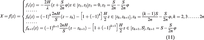
To verify the feasibility of the proposed parametric approach in equation (11), nine different parameter combinations were defined and tested, whose results were presented in Figure 9. It can be found out that the design schemes can be changed greatly by choosing different design parameters. And most importantly, they can be controlled with a united manner by equation (11), which would be beneficial for the quantitative investigation and optimization next.

Figure 9.

Diversity verification of the parametric approach.

A bionic noise reduction strategy

The serrated treatment of the trailing edge established on the bionic noise reduction technology was then carried out with the optimization. As shown in Figure 10, the optimization process consisted of the Central Composite Design (CCD) sampling method, the numerical methodology, the approximate model, and the Response Surface Method (RSM) analysis, etc. The detailed approach for each part would be introduced next.

Figure 10.

Flow chart of bionic noise reduction strategy.

Sampling with central composite design

As a typical sampling methodology for the Design of Experiment (DOE), CCD can provide almost as much information as the three-level factorial design with fewer tests.²⁸ Especially for three design parameters in DOE, the predicating model can be effectively established by estimating the effects of the design parameters and the corresponding response surfaces.²⁹ Hence, the sampling with CCD was utilized in this paper.

First, the upper and lower limits of all design variables were defined in Table 2. As the fixed variables of C and S, their specific values were the same as the experiment. And then, for the other changeable variables of H, n, and φ, the ranges of their values were set with consideration of processing and manufacturing, for that the bad models with the sharp trailing edges can be easily gotten without previously considerable thought.

Table 2.

Parameter values.

	Parameters	Values
Fixed values	Chord length (C)	100 mm
Fixed values	Span length (S)	200 mm
Variable values	Serrate tip-to-root distance (H)	[3.61 mm,15.39 mm]
	Serrated number (n)	[0.93,16.07]
	Install location adjustment factor (φ)	[0.03,0.97]

The design parameters were then coded, whose corresponding expressions were listed in Table 3. With the coded expressions in the table, the calculated design parameters were listed in Table 4, where 0 is the center point of the design space (the midpoint of each design variable range) and $α$ is taken as 1.6818 unit (the unit is the distance between 0 and 1) in this paper.

Table 3.

Relationship between coded and design variable.

Code	Value of variables
$- α$	$X_{\min}$
–1	$[(X_{\max} + X_{\min}) / 2] - [(X_{\max} - X_{\min}) / 2 α]$
0	$(X_{\max} + X_{\min}) / 2$
1	$[(X_{\max} + X_{\min}) / 2] + [(X_{\max} - X_{\min}) / 2 α]$
$α$	$X_{\max}$

X_min: the minimum value of each parameter; X_max: the maximum value of each parameter.

Table 4.

Design parameters and coded in CCD.

Items	Coded variable levels
	–1	0	1	$- α$	$α$
$H$	6	9.5	13	3.61	15.39
$n$	4	8.5	13	0.93	16.07
$φ$	0.22	0.5	0.78	0.03	0.97

H: serrate tip-to-root distance, n: serrated number, φ: install location adjustment factor.

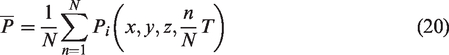
After coding the design parameters, the design matrix was determined. Twenty sets of design combinations were shown in the first four columns of Table 5. According to the design parameters, the bionic airfoils for each condition were constructed via the proposed parametric approach in “The parametric approach” section. Then the sound fields were calculated with the unsteady numerical methodology in “Validation of the numerical methodology” section. To reduce the target points, four representative sound field points (P1–P4 of Figure 4) were selected. Finally, the calculation results of OASPL were shown in the last four columns of Table 5.

Table 5.

The samples in the database with CCD.

No.	Coded levels			P1 (dB)	P2 (dB)	P3 (dB)	P4 (dB)
No.	$H$	$n$	$φ$	P1 (dB)	P2 (dB)	P3 (dB)	P4 (dB)
S1	–1	1	1	35.65	35.28	62.54	62.53
S2	0	$- α$	0	36.72	36.45	61.99	61.97
S3	–1	–1	1	36.41	36.22	63.95	63.94
S4	–1	1	–1	36.43	36.43	63.27	63.25
S5	1	1	1	36.82	36.50	62.49	62.51
S6	0	0	0	37.90	38.23	65.39	65.39
S7	0	0	0	37.90	38.23	65.39	65.39
S8	0	0	0	37.90	38.23	65.39	65.39
S9	1	–1	1	39.16	39.48	63.94	63.97
S10	0	0	0	37.90	38.23	65.39	65.39
S11	–1	–1	–1	35.26	35.14	62.27	62.30
S12	0	$α$	0	35.96	35.89	63.90	63.91
S13	1	–1	–1	37.23	38.03	63.12	63.10
S14	$- α$	0	0	35.62	35.46	63.10	63.11
S15	0	0	$α$	36.93	37.04	63.25	63.23
S16	0	0	$- α$	36.58	36.52	64.87	64.86
S17	0	0	0	37.90	38.23	65.39	65.39
S18	0	0	0	37.90	38.23	65.39	65.39
S19	1	1	–1	36.26	36.31	63.72	63.72
S20	$α$	0	0	37.08	37.41	61.46	61.45

H: serrate tip-to-root distance, n: serrated number, φ: install location adjustment factor; P1, P2, P3, P4: sound field point at P1, P2, P3, and P4 in Figure 4.

Establishment of the approximate models

The approximate models were used to establish the mathematical relationship between the performances and the design parameters. Currently, there are many approximate models, such as the Radial Basis Method, the Response Surface Method (RSM), the Kriging Method, etc. The RSM was a simple and relatively accurate approximate model to predict the mathematical relationships, which was widely applied in acoustics.³⁰ Especially, the second-order polynomial function model was suitable for the situation with three design parameters.³¹ Therefore, the RSM was adopted as the approximate model in this paper, which can be expressed as

{\hat{y}}_{i} = β_{0} + \sum_{i = 1}^{3} β_{i}^{j} X_{i} + \sum_{j = 1}^{3} β_{i i}^{j} {(X_{i})}^{2} + \sum_{i \neq j} β_{i k}^{j} X_{i} X_{k}

(12)

where

{\hat{y}}_{i}

is the predicted OASPL value of the four monitoring points P1–P4, and in the following equations, the corresponding is P1, P2, P3, P4;

X_{i}

X_{k}

are the design variables

N

n

φ

;

β_{0}

β_{i}^{j}

β_{i i}^{j}

β_{i k}^{j}

are the coefficients whose values can be determined through the fitting.

Aiming at the design variables and their corresponding calculated performances in Table 5, the established approximate models for the four monitoring points P1–P4 in Figure 4 were finally settled down as

\begin{array}{l} P 1 = 26 .98453 + 1 .05452 \times H+0 .83563 \times n +5 .6826 \times φ -0 .029503 \times H \times n +0 .2714239 \times H \times φ \\ -0 .32958 \times n \times φ -0 .040455 \times H^{2} -0 .024534 \times n^{2} -4 .5487737 \times φ^{2} \end{array}

(13)

\begin{array}{l} P 2=24 .64162 + 1 .32835 \times H +1 .05346 \times n +7 .26786 \times φ -0 .040118 \times H \times n +0 .2202561 \times H \times φ \\ -0 .3493899 \times n \times φ -0 .046173 \times H^{2} -0 .032529 \times n^{2} -5 .7514617 \times φ^{2} \end{array}

(14)

\begin{array}{l} P 3=51 .52297 + 1 .71982 \times H+0 .87032 \times n +10 .3716 \times φ -0 .00347302 \times H \times n - 0.1736487 \times H \times φ \\ -0 .4450797 \times n \times φ -0 .086073 \times N^{2} -0 .040463 \times n^{2} -5 .5101384 \times φ^{2} \end{array}

(15)

\begin{array}{l} P 4 = 51 .61241 + 1 .70957 \times H +0 .86630 \times n +10 .314 \times φ -0 .00305714 \times H \times n -0 .1628739 \times H \times φ \\ -0 .4427001 \times n \times φ -0 .085995 \times H^{2} -0 .040590 \times n^{2} -5 .5766475 \times φ^{2} \end{array}

(16)

To verify the accuracy of the settled approximate models, the coefficient of determination (R²) was calculated according to Gunst,³² which can be expressed as

R^{2} = 1 - \frac{S S_{residual}}{S S_{tatal}} = 1 - \frac{\sum_{i = 1}^{n} {(y_{i} - {\hat{y}}_{i})}^{2}}{\sum_{i = 1}^{n} {(y_{i} - \bar{y})}^{2}}

(17)

where

S S_{residual}

is the sum of square of residuals, and the residual is the difference between the actual value (

y_{i}

) and the predicted value (

{\hat{y}}_{i}

);

S S_{total}

is the total sum of squares, which is calculated by summing the squares of difference between the actual value (

y_{i}

) and the mean value (

{\bar{y}}_{i}

A fitted model should have a minimum value of 0.8.³³ In this paper, the values of R² for the above fitting formulas were 0.90, 0.91, 0.90, and 0.90, respectively. The minor errors between the predicted value and the actual value were given in Figure 11. From the figure, it can be concluded out that the calculated approximate models are rather accurate and available.

Figure 11.

Errors between predicted values and actual values: (a) sound field point at P1, (b) sound field point at P2, (c) sound field point at P3, and (d) sound field point at P4.

Response surface method analysis

According to the calculated approximate models and the fitting process with RSM, the respond surfaces were settled down to predict the noise values with different design parameters. Figure 12 showed the impact of three variables on noise reduction.

Figure 12.

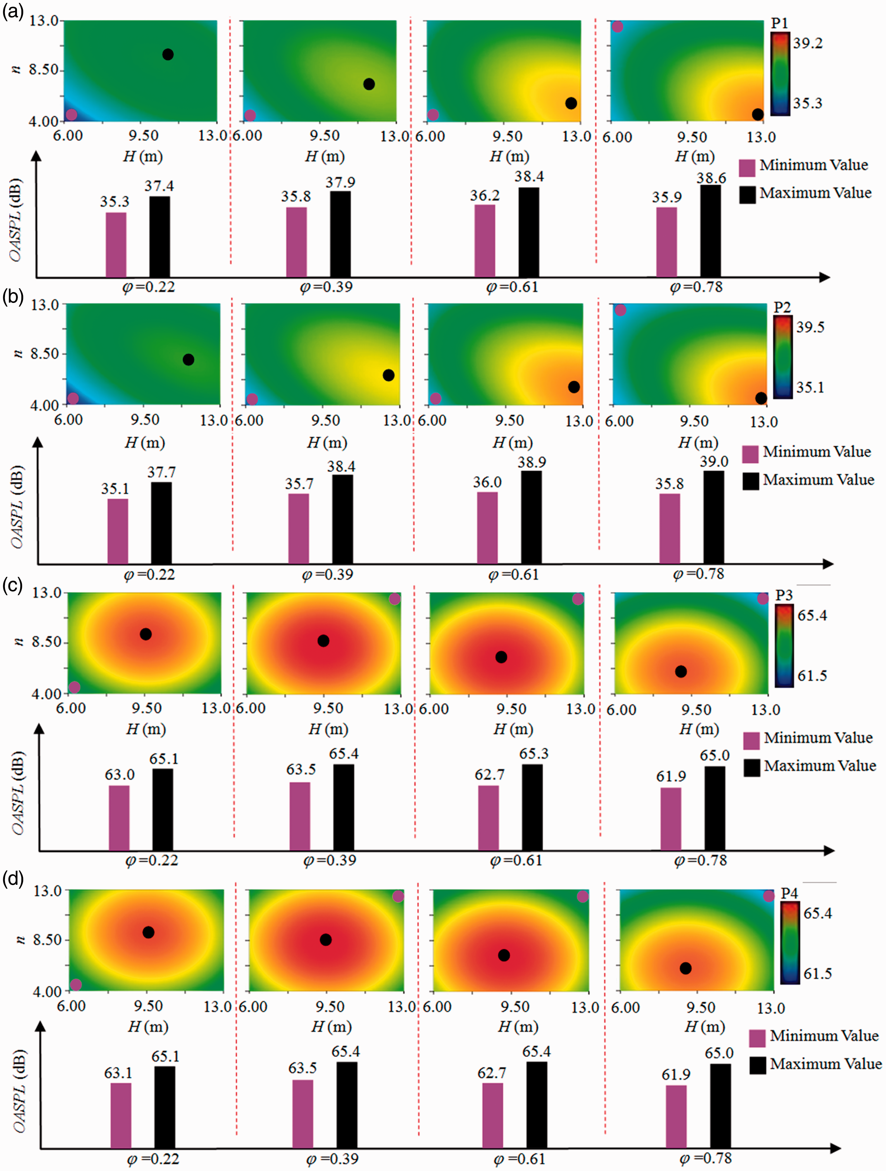
Results of respond surface determined by the design parameters: (a) respond surface for OASPL at P1, (b) respond surface for OASPL at P2, (c) respond surface for OASPL at P3, and (d) respond surface for OASPL at P4.

For the install location adjustment factor φ, it can affect the noise level. Additionally, when the values of the serrate-to-root distance H and the serrated number n are different, the optimal value of the install location adjustment factor isn’t fixed. Therefore, proposing the install location adjustment factor is significant and necessary.

As presented in Figure 12(a) and (b), the noise distributions at the front and rear location of P1 and P2 were analyzed at first. Regarding the minimum OASPL zones, when the install location adjustment factor increases, the corresponding determined serrated number would have an increasing trend. However, the specific values for the minimum OASPL zones would firstly increase and then decrease under different install location adjustment factors. For the noise at P1 and P2, by predicting and analyzing the distributing performances under different design variables, the optimal design variables were approximate as: H ∈ [6, 6.5], n ∈ [4, 5], and φ ∈ [0.22, 0.28].

As shown in Figure 12(c) and (d), the noise distributions were then analyzed at the upper and lower location of P3 and P4. For the minimum OASPL zones, as the install location adjustment factor increases, there would be an increasing trend for both of the corresponding determined serrate-to-root distance and serrated number. However, the specific values for the minimum OASPL zones would firstly increase and then decrease with the increase of the install location adjustment factors. For the noise at P3 and P4, with the predicted noise analyzed under different design variables, the optimal design variables were approximate as: H ∈ [12.5, 13], n ∈ [12, 13], and φ ∈ [0.72, 0.78].

In terms of the contradiction between Gruber¹⁵ and Moreau¹⁶ illustrated in Part 1, the explanation can be concluded as: aiming at the noise value controlled by the ratio of the serrated number to the serrate-to-root distance, the noise value would take a decreasing trend when the ratio is smaller or larger than the black point in Figure 12, so that the contradictory conclusions could be drawn by choosing different analysis zones. Therefore, a global quantitative analysis of the effects of design parameters on the airfoil’s noise is necessary.

Additionally, the ranges for the optimal design parameters at the monitoring P1–P4 points were not completely the same, but the noise values of P3 and P4 are much larger than the values of P1 and P2. Thus, the noise optimization of P3 and P4 were taken as the main focus, and the optimal design parameters’ ranges were suggested to choose: H ∈ [12.5, 13], n ∈ [12, 13], and φ ∈[0.72, 0.78].

Noise analysis

The sensitivity of the install location adjustment factor

Taking into account the existence of the casing or wall near the span-end of the airfoil, the install location adjustment factor was proposed. To analyze the sensitivity of the install location adjustment factor, three sets of serrated trailing edges were selected in Figure 13. The selected models were executed by the numerical method above, and the sound power level (PWL) was analyzed, which is directly related to the value of the sound source

PWL = 10 \lg (\frac{W}{W_{ref}})

(18)

where W_re_f is the reference sound power, whose value is 1 × 10⁻¹² W; W is the sound power.

Figure 13.

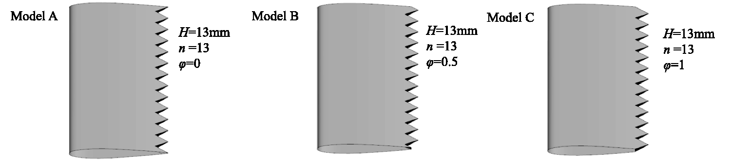
Models with different install location adjustment factors.

The sound power level spectrum with different install location adjustment factors is given in Figure 14. It can be seen that the install location adjustment factor has an influence on the maximum frequency of the PWL. Additionally, the spatial distribution of the sound field is calculated by the boundary element method (BEM). By comparing the BEM and the FW-H equation, Zhang et al.³⁴ found out that the difference between the numerical results of these two methods was rather small at the far sound field location. So the BEM is used to analyze the spatial distribution of the sound field. The sound field is determined as a sphere, whose center is the airfoil’s centroid with a 1.0 m radius. Therefore, combining the frequency spectrum and the SPL contours at the maximum of each model, the airfoil self-noise of model C is larger than that of model A and model B. Overall, for the research on the serrated trailing edge of an airfoil with casing or wall, the install location adjustment factor should be considered

Figure 14.

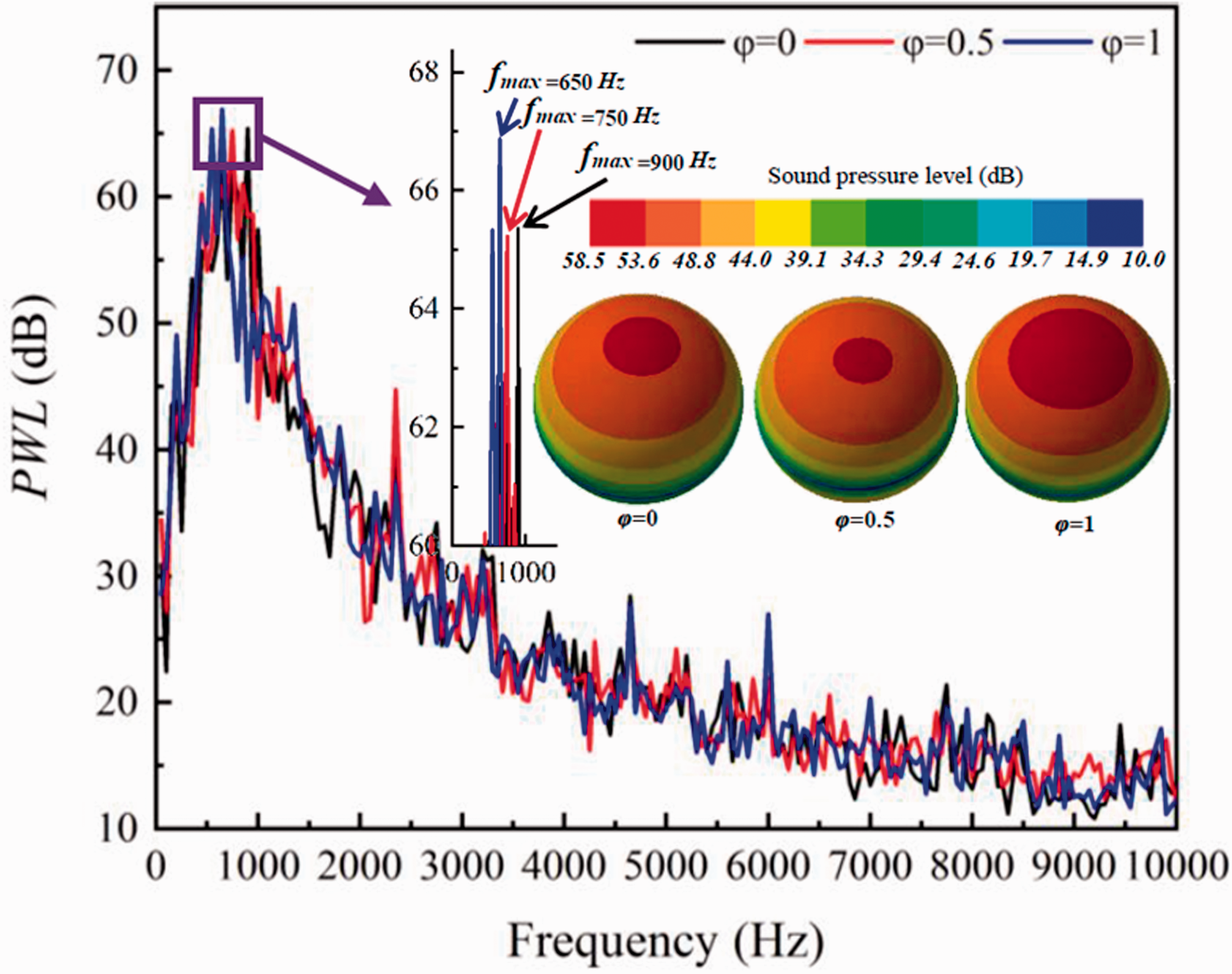
Frequency spectrum and the SPL contours.

The noise characteristics

After executing the bionic noise reduction process in Figure 10, the optimal result is obtained with RMS. To further illustrate the feasibility of the serrated treatment approach, the comparative analysis between the reference model and the optimized bionic model would be implemented next.

With the identified optimized parameters (H = 13 mm, n = 13, φ = 0.78), the corresponding optimized bionic model is configured. Under the same settings in “Validation of the numerical methodology” section, the noise performances of the reference model and the optimized bionic model are simulated. The sound field simulation results at all monitoring points in Figure 4 were presented in Figure 15. It can be clearly seen that the optimized bionic model can effectively reduce the OASPL by 2 dB approximately.

Figure 15.

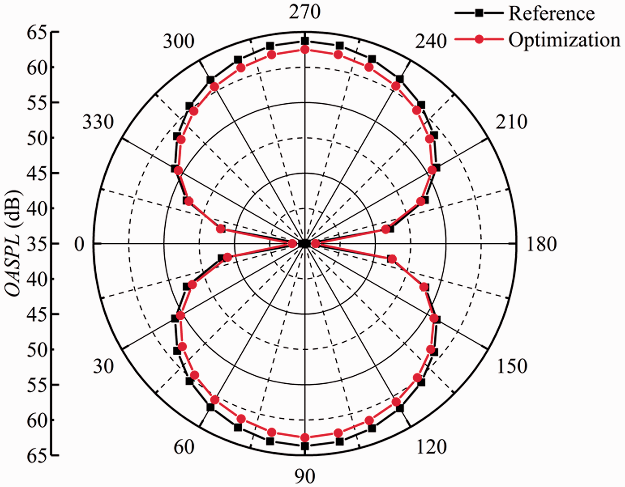
Comparison of the OASPL between the reference and the optimized model.

To further illustrate the effect of the serrated trailing edges on noise reduction, the Sound Pressure Level (SPL) at different frequencies would be analyzed. The SPL can be calculated as

SPL = 20 \lg (\frac{P_{e}}{P_{ref}})

(19)

where p_re_f is the reference pressure, whose value is 2 × 10⁻⁵Pa (for air); p_e is the effective sound pressure.

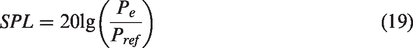
Figure 16 shows the calculated SPL changing with different frequencies at P3 and P4. Presented in the figure, it can be noted that the discrete tones in the hump-shaped broadband noise are an important characteristic of the airfoil noises. This phenomenon agrees well with Nakano et al.¹⁹ According to the spectral characteristics, the noise could be attributed to the laminar boundary layer instability noise. As the box enlarged in Figure 16, in the hump-shaped spectra, the tone peak is a superposition based on the broadband contribution centered on the main frequency f_s and a set of discrete frequencies f_n. For the optimized bionic model, under the hump-shaped broadband noise (1000–3500 Hz), the SPL can be significantly reduced. Therefore, the noise at the low-medium frequency can be suppressed by the serrated trailing edge, which satisfies with the validating experiment of Zhang.³⁵

Figure 16.

Comparison of the SPL between the reference and the optimized model: (a) sound pressure levels at P3 and (b) sound pressure levels at P4.

The corresponding sound field distributions are presented in Figure 17. The direction of noise propagation is mainly toward the upper and lower airfoil, so the noise of the spatial sound field has a dipole directivity, which is consistent with the conclusion of Ramirez et al.³⁶ In Figure 17, the SPL values directly reflect the effectiveness of the serrated trailing edge.

Figure 17.

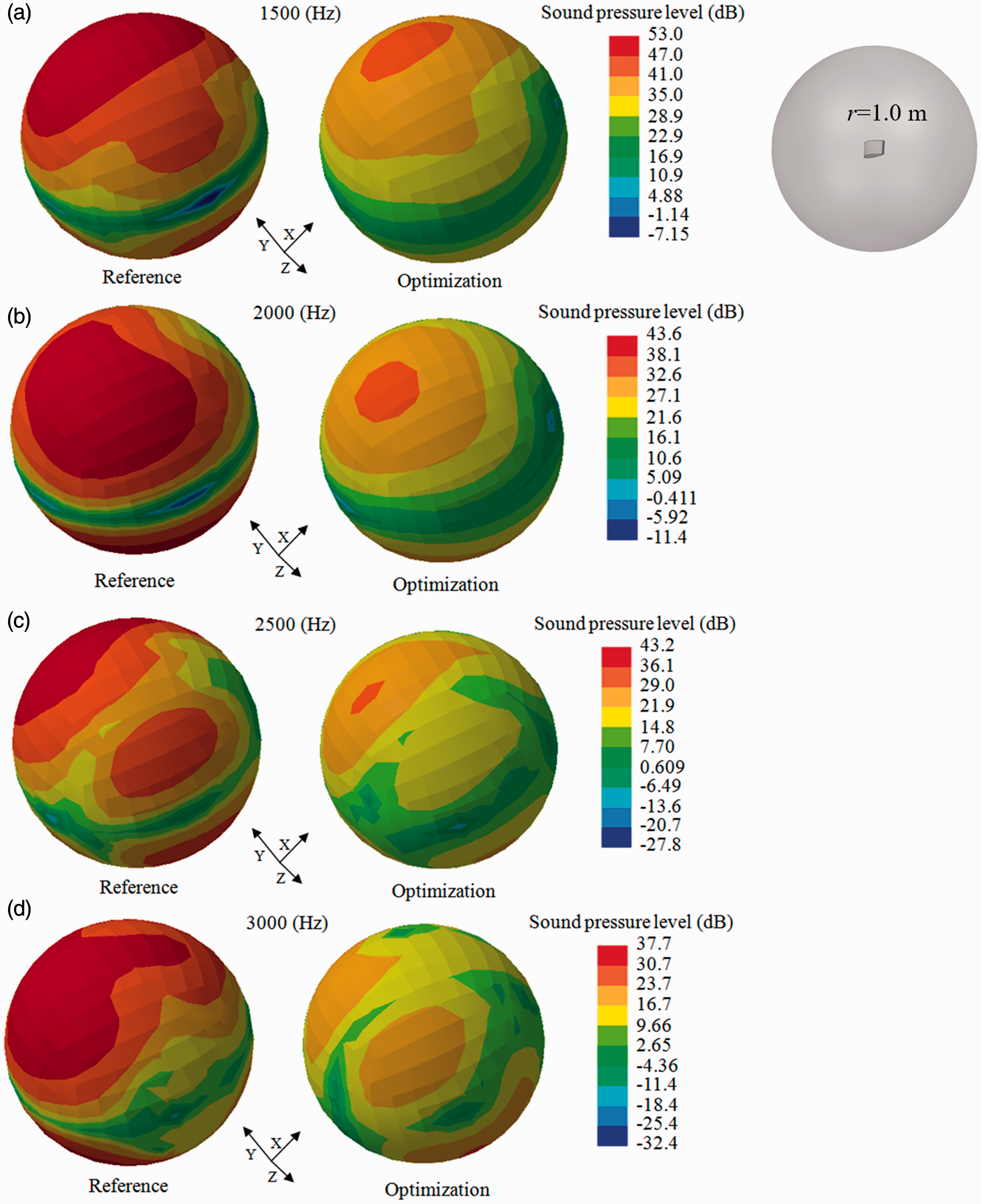
Spatial distribution of sound field between the reference and the optimized model: (a) sound pressure level at 1500 Hz, (b) sound pressure level at 2000 Hz, (c) sound pressure level at 2500 Hz, and (d) sound pressure level at 3000 Hz.

Since the sound pressure level is limited by the spatial position, the sound power level (PWL) is analyzed to further verify the above results. The sound power level is presented in Figure 18. It can be found that the value of the sound source with the optimized model is lower in the dark areas and the PWL is reduced by about 10 dB at the low-medium frequency. Eventually, the bionic noise reduction strategy is verified.

Figure 18.

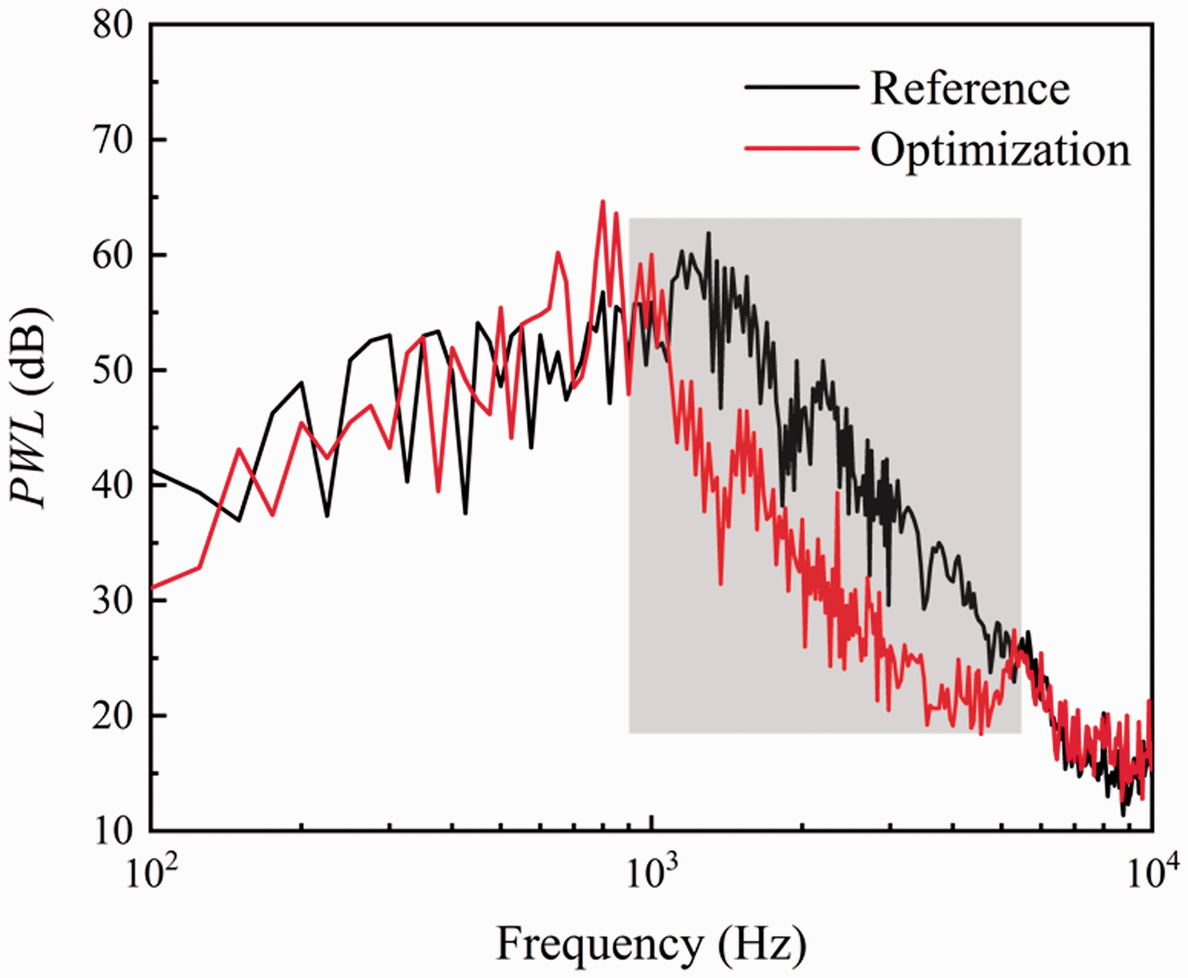
Comparison of the PWL between the reference and the optimized model.

Analysis of the noise reduction mechanism

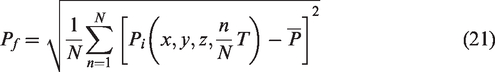
In “The sensitivity of the install location adjustment factor” section, it has been seen that the noise belongs to the dipole noise. For the dipole noise, it’s related to pressure fluctuation on the airfoil surface.³⁶ To analyze the noise influence mechanism of the install location adjustment factor, an innovative method of the unsteady evaluation is executed, which is the pressure fluctuation intensity. The pressure fluctuation intensity is calculated as³⁷

\bar{P} = \frac{1}{N} \sum_{n = 1}^{N} P_{i} (x, y, z, \frac{n}{N} T)

(20)

P_{f} = \sqrt{\frac{1}{N} {\sum_{n = 1}^{N} [P_{i} (x, y, z, \frac{n}{N} T) - \bar{P}]}^{2}}

(21)

where

P_{f}

is the pressure fluctuation intensity;

\bar{P}

is the time-mean pressure;

P_{i}

is the pressure at the netted nodes; T is the sampling time, T = 0.1 s; N is the sampling quantity in the sample, in this paper N = 100.

For the different install location adjustment factors, the pressure fluctuation intensity contours of the airfoil surface are presented in Figure 19. It can be found that the pressure fluctuation intensities of the near-wall serration are different and the pressure fluctuation intensities of the far-wall serration are the same. Therefore, it can be indicated that the install location adjustment factor mainly affects the near-wall flow field of the serrated trailing edge.

Figure 19.

Pressure fluctuation intensity contours of different install location adjustment factors.

To further analyze the influence of the near-wall flow field of the serrated trailing edge, the vorticity that can indicate the position and strength of the vortex is calculated as

Ω_{x} = \frac{\partial w}{\partial y} - \frac{\partial v}{\partial z}

(22)

where

Ω_{x}

is x-direction vorticity;

v

is y-direction velocity;

w

is x-direction velocity.

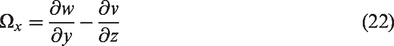
According to the equation, the x-direction vorticity contours of different install location adjustment factors are shown in Figure 20(a) to (c), respectively, describe the spanwise section at vale, middle, and crest of the serrated trailing edge. As shown in Figure 20(a), the distributions of the near-wall vorticity are the same, and due to the influence of the wall, the corner vortices (in the red box) are found near the wall. In Figure 20(b) and (c), as the chord position changes, the corner vortices would diffuse along the spanwise direction. From the purple box, it can be seen that the third structure (φ = 1) has the largest vorticity near the wall, which is caused by the size of the area formed by the wall and serration. The install location adjustment factor is one of the factors affecting airfoil self-noise.

Figure 20.

Vorticity contours of different install location adjustment factors: (a) spanwise section at vale, (b) spanwise section at middle, and (c) spanwise section at crest.

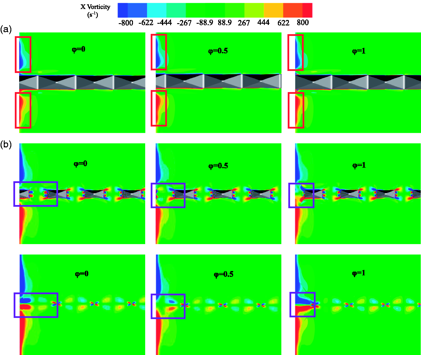
For the noise reduction mechanism of the serrated trailing edge, firstly, the monitoring points at the serrated trailing edge are defined in Figure 21(a), which are vale (A1), middle (A2), and crest (A3), and the monitoring point at the primitive trailing edge is defined as N1 in Figure 21(b).

Figure 21.

Monitoring points at serrated trailing edge: (a) serrated trailing edge and (b) normal trailing edge.

Then the pressure pulsations at different monitoring points are calculated in Figure 22(a). The pressure pulsation increases from the vale to the crest. Besides, the pressure pulsations at A1 and A2 were lower than A3 and N1, and the pressure pulsations at A3 and N1 have a minor difference. Overall, the bionic structure can reduce the pressure pulsation at the trailing edge.

Figure 22.

Pressure pulsation: (a) pressure pulsation at different time-step and (b) pressure fluctuation intensity.

To further prove the above conclusions and avoid the random problem caused by the selection of monitoring points, the pressure fluctuation intensity is given in Figure 22(b).The comparison results of the pressure fluctuation intensity for different models are shown in Figure 22(b). The chord distribution of the pressure fluctuation intensity is related to the trailing edge: the traditional airfoil is uniform, while the bionic airfoil is serrated distributed. To further analyze, the purple box is enlarged in Figure 22(b). For the near-tail region, the pressure fluctuation intensity of the bionic airfoil is reduced. For the trailing edge region, the pressure fluctuation intensity is also improved through the bionic structure, whose result is in line with Figure 22(a). According to the FW-H equation, when the pressure pulsation decreases, the dipole sound source is attenuated. To further explore the mechanism of pressure pulsation reduction, the flow field near the trailing edge would be continually analyzed.

The streamlines and chord velocity contours are given in Figure 23. In Figure 23(a), for the low Reynolds number and the airfoil with zero angle of attack, the separation bubbles (marked in red circle) would appear in the near-tail region, which would cause the separation of the laminar boundary layer. According to the research of Desquesnes et al.,³⁸ the boundary layer separation along the airfoil chord can lead to an unstable shear layer with T–S (Tollmien–Schlichting) instability waves, and a dipolar acoustic source can be formed through the interaction of the T-S waves and the trailing edge. The existence of separation bubbles can amplify the trailing edge vortex (marked in yellow circle), and the vortex shedding noise would show the discrete tonal distribution characteristics. For the serrated trailing edge in Figure 23(b), due to the increased TE (Trailing Edge) thickness at the vale, the large-scale shedding vortex is also existent even if there is no obvious separation bubble. Hence, under this condition, the bionic airfoil self-noise is also discrete tonal distribution characteristics.

Figure 23.

Streamlines and chord velocity contours: (a) normal airfoil and (b) bionic airfoil.

As shown in Figure 23(b), the bionic airfoil can result in the smaller hump-shaped broadband noise, in terms of the smaller separation bubbles in the near-tail region and the weaker T-S instability waves, than the normal airfoil. Then, to analysis the changes of the separation bubbles, the contours of flow fields at different times are given in Figure 24. For the normal airfoil, the scale of separation bubbles would be larger over time, and there would be the shedding vortex at the trailing edge when the separation bubbles expanded to any degree in Figure 24(a). For the bionic airfoil, it can be seen from the chord section at A3 that the separation bubbles are also existent, however the separation bubbles would shrink and disappear over time, which makes T-S instability waves weaker.

Figure 24.

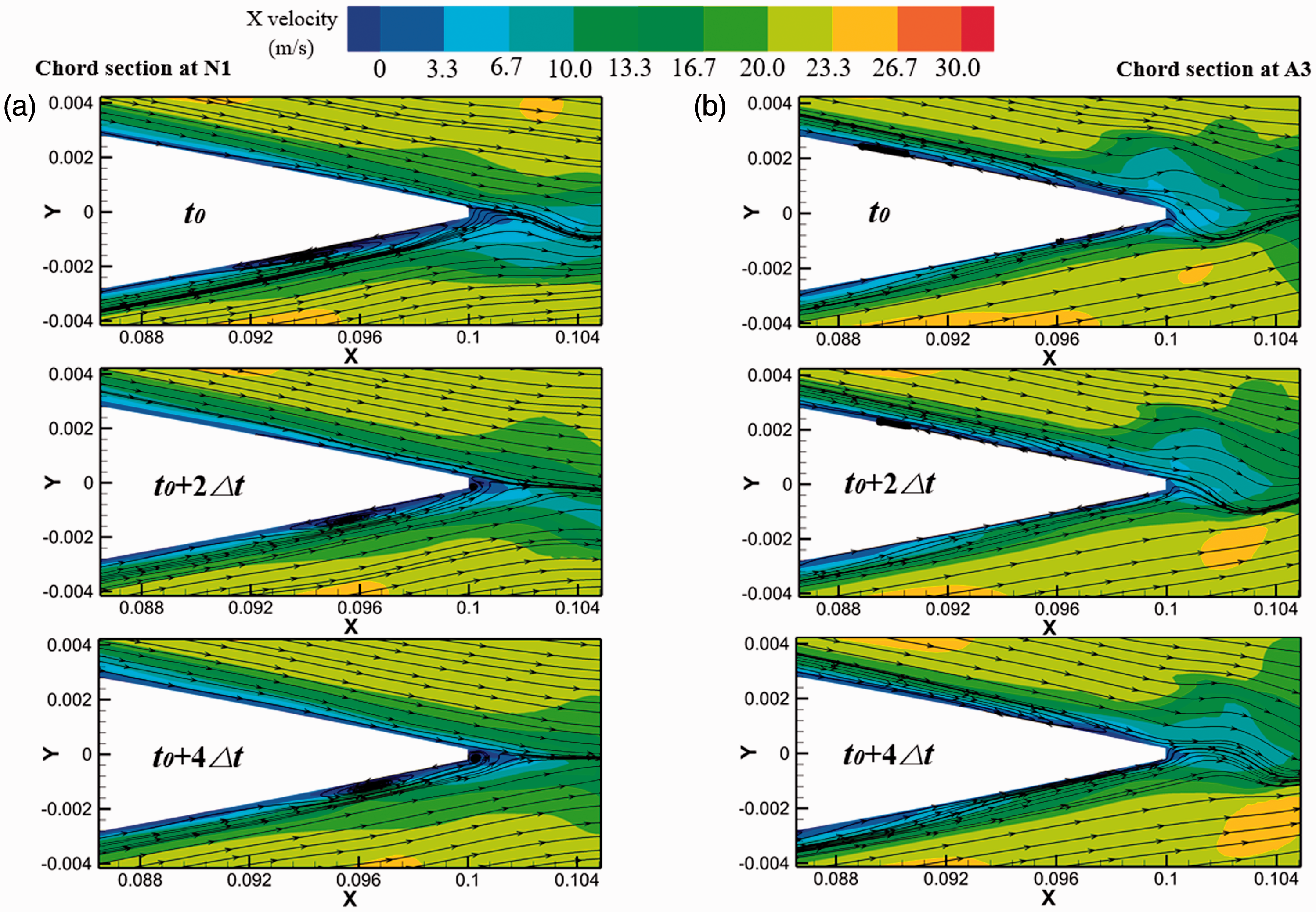
Contours of the flow fields at different times: (a) normal airfoil and (b) bionic airfoil.

In Figure 25(a), Chong et al.¹⁸ assumed that the edge vortices appeared at the serrated trailing edge, which suppressed the separation bubbles at the trailing edge. According to Figure 25(b), the streamline distribution is the same as Chong’s hypothesis. Due to the appearance of the edge vortices, it can be known that the spanwise velocity is generated at the near-tail surface, which would destroy the growth of separation bubbles along the chord direction. Regarding the formation of the edge vortices, the pressure and streamline distribution around the middle of serration are analyzed.

Figure 25.

Streamline figures: (a) the hypothetical schematic diagram by Ching et al.¹⁸ and (b) the streamlines around serration.

Figure 26(a) shows the partial enlarge drawing of the streamline around the serration. It can be seen that there would exist a pair of reverse edge vortices that can suppress the development of the laminar separation bubbles near the trailing edge of both surfaces. As enlarged in Figure 26(b), the serrated structure would cause a low-pressure zone near the trailing edge, which would lead to the spanwise velocity. Moreover, the mainstream is still flowing along the chord direction, so the edge vortices are formed. Overall, the serrated trailing edge can affect the development of the laminar separation bubbles to achieve the reduction of the hump-shaped broadband noise.

Figure 26.

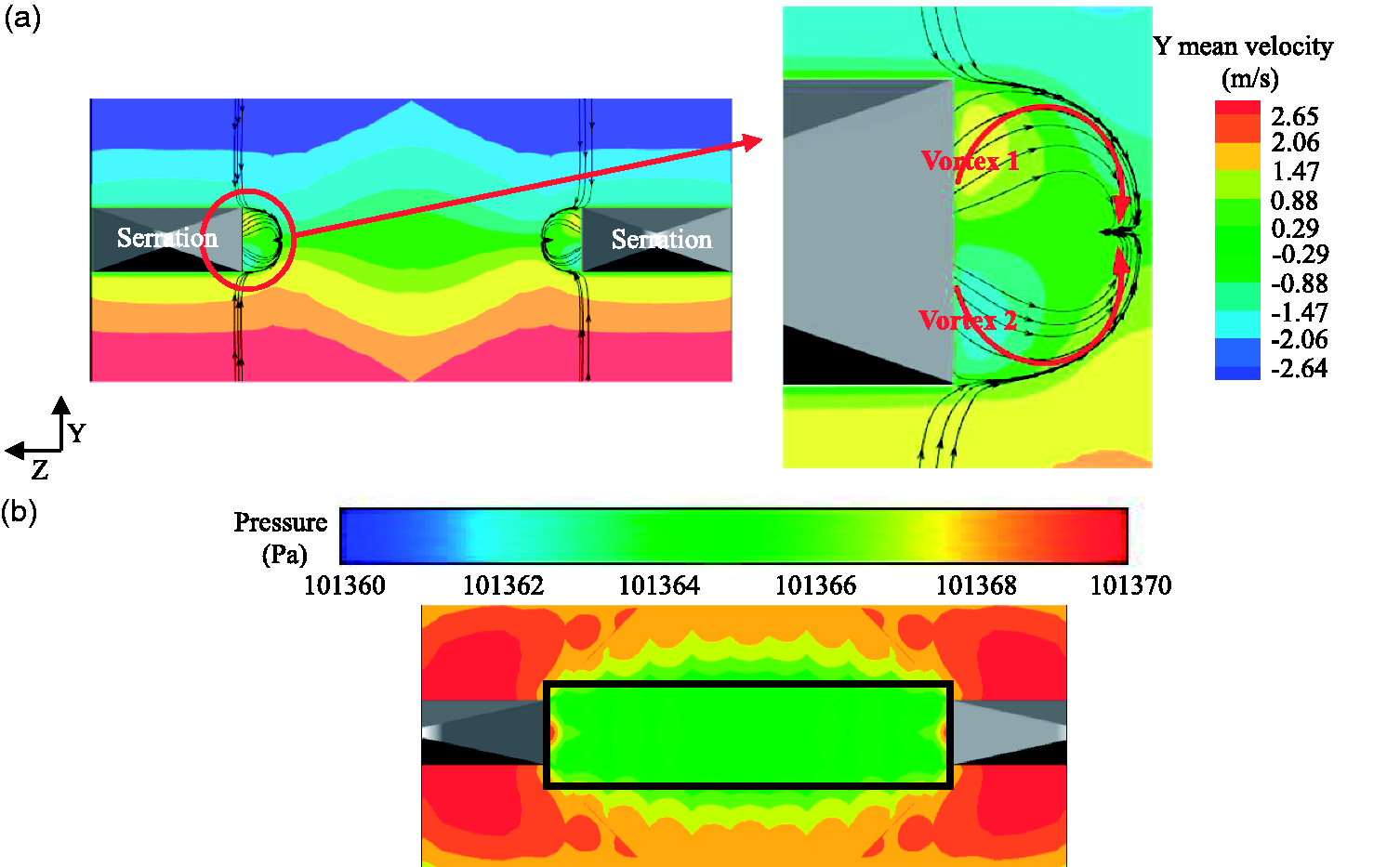
Pressure and streamline distribution around the middle of serration: (a) the streamlines distribution and (b) the pressure distribution.

Conclusions

To make up for the lack of adjusting the install location of the serration on the trailing edge and analyze the distributing laws controlled by the design variables, a bionic noise reduction strategy on the trailing edge was proposed. Taking the typical NACA0018 as the study target, the optimal design scheme was obtained and the corresponding bionic noise reduction mechanism was explained. Besides, the contradictory conclusions in previous studies were clarified.

The following conclusions can be gotten as:

A united parametric design approach is proposed to generate different design schemes. Based on the serrate tip-to-root distance and the serrated number proposed by previous studies, the install location adjustment factor is defined and imported in this study. It’s proved that the install location adjustment factor affects the reduction of noise.

With the integration of the Central Composite Design (CCD) and other methods, a bionic noise reduction strategy is established and the reliability of each process is evaluated and demonstrated. The successful obtain of the optimal bionic airfoil illustrates the effectiveness of the integrated noise reduction strategy.

The optimal serrated trailing edge structure is finally settled down. Through the respond surface and sound filed analysis, it can be found as:

When the values of the serrate-to-root distance and the serrated number are different, the optimal value of the install location adjustment factor isn’t fixed;

The noise value would take a decreasing trend when the ratio is smaller or larger than a special point, which can clarify the previous contradictory conclusions between Gruber and Moreau;

The optimized bionic model can effectively reduce the overall sound pressure level by about 2 dB.

The noise reduction mechanism is analyzed. Taking into account the existence of the casing or wall near the span-end of the airfoil, the install location adjustment factor mainly affects the near-wall flow field of the serrated trailing edge. The edge vortices appear resulting from the low-pressure zone at the serrated trailing edge, which can suppress the laminar separation bubbles, so the pressure pulsations are significantly reduced near the serration. As a result, the noise is reduced with the adoption of the serrated trailing edge.

Footnotes

Declaration of conflicting interests

The author(s) declared no potential conflicts of interest with respect to the research, authorship, and/or publication of this article.

Funding

The author(s) disclosed receipt of the following financial support for the research, authorship, and/or publication of this article: This study was co-supported by National Natural Science Foundation of China (Grant 52005073); National Science and Technology Major Project (Grant 2018YFB0606100); National Basic Research Program of China (Grant 2015CB057301) and Research and Innovation in Science and Technology Major Project of Liaoning Province (Grant 2019JH1-1010024).

ORCID iDs

Haoran Liu

Xiaofang Wang

References

Koca

Genç

Açıkel

, et al. Identification of flow phenomena over NACA 4412 wind turbine airfoil at low Reynolds numbers and role of laminar separation bubble on flow evolution. Energy 2018; 144: 750–764.

Emilio

CC.

Workshop: atmospheric and ground effects on aircraft noise. Int J Aeroacoust 2014; 13: 1–3.

Gao

Zheng

, et al. Experimental investigation on static/dynamic characteristics of a fast-response pressure sensitive paint. Chin J Aeronaut 2018; 31: 1198–1205.

Martinez-Lera

Christophe

Schram

Computation of the self-noise of a controlled-diffusion airfoil based on the acoustic analogy. Int J Aeroacoust 2017; 16: 44–64.

Geyer

Sarradj

Fritzsche

Porous airfoils: noise reduction and boundary layer effects. Int J Aeroacoust 2010; 9: 787–820.

Leitch

Saunders

WF.

Reduction of unsteady stator-rotor interaction using trailing edge blowing. J Sound Vib 2000; 235: 235–245.

Oerlemans

Fisher

Maeder

, et al. Reduction of wind turbine noise using optimized airfoils and trailing-edge serrations. AIAA J 2009; 47: 1470–1481.

Howe

MS.

Noise produced by a sawtooth trailing edge. Acoust Soc Am J 1991; 90: 482–487.

Jones

Sandberg

RD.

Numerical investigation of airfoil self-noise reduction by addition of trailing edge serrations. In. 16th AIAA/CEAS aeroacoustics conference, Sweden, 2010.

10.

Carlos

Roberto

Daniele

Effect of trailing edge serration-flow misalignment on airfoil noise emissions. J Sound Vib 2017; 405: 19–33.

11.

Chong

Joseph

PF.

An experimental study of airfoil instability tonal noise with trailing edge serrations. J Sound Vib 2013; 332: 6335–6358.

12.

Moreau

Doolan

CJ.

Tonal noise from trailing edge serrations at low Reynolds number. In: 19th AIAA/CEAS aeroacoustics conference, Germany, 2013.

13.

Gruber

Joseph

Chong

On the mechanisms of serrated airfoil trailing edge noise reduction. In: 17th AIAA/CEAS aeroacoustics conference, USA, 2011.

14.

Lau

ASH

Xun

The control of aerodynamic sound due to boundary layer pressure gust scattering by trailing edge serrations. J Sound Vib 2018; 432: 133–154.

15.

Gruber

Azarpeyvand

Joseph

Airfoil trailing edge noise reduction by the introduction of sawtooth and slitted trailing edge geometries. In: Proceedings of 20th international congress on acoustics, Australia, 2010.

16.

Moreau

Doolan

CJ.

Noise-reduction mechanism of a flat-plate serrated trailing edge. AIAA J 2013; 51: 2513–2522.

17.

Lyu

Azarpeyvand

Sinayoko

Prediction of noise from serrated trailing-edges. J Fluid Mech 2016; 793: 556–588.

18.

Chong

Joseph

Vathylakis

, et al. On the noise and wake flow of an airfoil with broken and serrated trailing edges. In: 17th AIAA/CEAS aeroacoustics conference, USA, 2011.

19.

Nakano

Fujisawa

Lee

Measurement of tonal-noise characteristics and periodic flow structure around NACA0018 airfoil. Exp Fluid 2006; 40: 482–490.

20.

Garrec

Gloerfelt

Corre

A numerical insight into the effect of confinement on trailing edge noise. J Acoust Soc Am 2008; 123: 369–371.

21.

Fujisawa

Shibuya

Nashimoto

, et al. Aerodynamic noise and flow visualization around two-dimensional airfoil. Trans Vis Soc Jpn 2001; 21: 123–129.

22.

Kim

Lee

Fujisawa

Computation of unsteady flow and aerodynamic noise of NACA0018 airfoil using large-eddy simulation. Int J Heat Fluid Flow 2006; 27: 229–242.

23.

Ansys-Fluent Inc, 2008. Fluent user’s guide.

24.

Ducros

Franck

Poinsot

Wall-adapting local eddy-viscosity models for simulations in complex geometries. In: Proceedings of 6th ICFD conference on numerical methods for fluid dynamics, UK, 1998.

25.

Williams

JEF

Hawkings

DL.

Sound generation by turbulence and surfaces in arbitrary motion. Philos Trans R Soc London Ser A, Math Phys Sci 1969; 264: 321–342.

26.

Mendonca

Bonthu

Kim

Transitional flow and aeroacoustic prediction of NACA0018 at Re=1.6 × 105. In: 17th AIAA theoretical fluid mechanics conference, USA, 2013.

27.

Tong

Qiao

Chen

, et al. Broadband noise prediction using large eddy simulation and a frequency domain method. Appl Acoust 2017; 117: 94–105.

28.

Demirel

Kayan

Application of response surface methodology and central composite design for the optimization of textile dye degradation by wet air oxidation. Int J Ind Chem 2012; 3: 24–10.

29.

Park

SH.

Extension of central composite design for second-order response surface model building. Commun Stat 2010; 39: 1202–1211.

30.

Lafronza

Mcalpine

Keane

, et al. Response surface method optimization of uniform and axially segmented duct acoustics liners. J Aircr 2006; 43: 1089–1102.

31.

Wang

YM.

Optimization of the cross section area on the meridian surface of the 1400-MW canned nuclear coolant pump based on a new medial axial transform design method. Ann Nucl Energy 2018; 115: 466–479.

32.

Gunst

RF.

Response surface methodology: process and product optimization using designed experiments. Technometrics 1996; 38: 284–286.

33.

Lim

Beh

Ching

DLC

, et al. Central composite design (CCD) applied for statistical optimization of glucose and sucrose binary carbon mixture in enhancing the denitrification process. Appl Water Sci 2017; 7: 3719–3727.

34.

Zhang

Chen

Sun

GC.

Comparative study on the flow field and acoustic field simulation for noise prediction induced by the flow around a cylinder. Noise Vib Control 2016; 36: 26–31.

35.

Cheng

Qiao

Chen

, et al. An experimental study on the noise reduction with bionic airfoil. J Eng Thermophys 2018; 39: 2159–2170.

36.

Ramirez

Wolf

WR.

Effects of trailing edge bluntness on airfoil tonal noise at low Reynolds numbers. J Brazil Soc Mech Sci Eng 2015; 37: 1–12.

37.

Yang

Wang

, et al. A symmetrical-nonuniform angular repartition strategy for the vane blades to improve the energy conversion ability of the coolant pump in the pressurized water reactor. Nucl Eng Des 2018; 337: 245–260.

38.

Desquesnes

Terracol

Sagaut

Numerical investigation of the tone noise mechanism over laminar airfoils. J Fluid Mech 2007; 591: 155–182.