Blade retrofit design to reduce the noise of an axial flow fan by mitigating the tip leakage vortex

Abstract

In the context of controlling axial fan aerodynamic noise, one effective approach involves the redesign of the blade. In the present study, a novel blade design was formulated for a specific model of axial flow fan, targeting the mitigation of the tip leakage vortex (TLV) and subsequent reduction of noise levels. The assessed noise-reduction blades have perforations drilled from the leading edge (LE) to the pressure surface (PS) of the blades. By impeding the tip leakage flow (TLF), these perforations effectively weaken the TLV. The three-dimensional non-constant flow field within the channel is computed employing the shear stress transport (SST) turbulence model. The aerodynamic noise prediction, which is based on the Lighthill’s acoustic analogy theory, shows that the designed blades can effectively reduce the aerodynamic noise of the axial fan. Specifically, enhancing the ratio of inlet area to outlet area of the ventilation holes leads to an improved noise reduction effect. Notably, for ratios of 0.44 and 1.06, the designed blades exhibit noise reductions of up to 3.3 dB(A) and 3.9 dB(A), respectively. Meanwhile, the static efficiency of these two fans is reduced by 0.50% and 0.26%, respectively. The study thus provides good theoretical support for the design of axial flow fans in the context of noise reduction.

Keywords

Axial flow fan aerodynamic noise numerical prediction blade design tip leakage vortex noise reduction

Introduction

The generation of airflow is facilitated by an axial fan, which serves as a mechanical device extensively utilized in diverse applications such as conveying ventilation, cooling, heating, and others. However, the noise emitted by axial fans within ventilation systems has garnered significant interest due to increasing concerns pertaining to health and the environment. Consequently, there has been a growing focus on noise reduction strategies associated with axial fans.

In axial fan noise studies, tonal noise and broadband noise are encompassed, with tonal noise primarily manifesting at the Blade Passing Frequency (BPF) and its harmonics.¹ Scholars have directed their research focus towards tonal noise, as it governs the overall sound pressure level (OSPL). The rotor-stator interaction (RSI) has been identified by Tyler et al.² as the primary source of tonal noise, and they have proposed the RSI theory. Furthermore, it also has been indicated that tonal noise is significantly influenced by RSI.^3,4 The conclusion was reached by Laurent Soulat et al.⁵ through numerical analysis of Counter-Rotating Open Rotors that the wakes and tip vortex of the front rotor strike the aft rotor, resulting in strong interaction on the surface of the aft rotor. It was suggested that maintaining a certain distance between the front and aft rotors is imperative for mitigating interference noise. Besides, it was also found through research by Fabio Casagrande Hirono et al.⁶ that tonal noise was produced by the interference of the wake of the front rotor with aft rotor, and they suggested that the spacing between the front and aft rotors should be increased. Hence, optimizing the rotor-stator spacing leads to improved noise reduction.^7–9 Moreover, several strategies have been identified to mitigate RSI and, consequently, tonal noise. These include employing an appropriate number of blades,¹⁰ managing blade inhomogeneity,^11–13 and optimizing the blade swept shape.^14,15 Nevertheless, it is crucial to maintain the axial fan’s structural integrity in accordance with aerodynamic performance requirements, limiting the flexibility to arbitrarily alter the mentioned structural parameters.

In the case where the turbine structure has been determined, greater interest lies in achieving noise reduction. The role of rotor-wake-stator interaction in influencing tonal noise has been emphasized by Han et al.⁸ In accordance with the principles of aerodynamic acoustics, noise reduction commonly involves modifying blade design to suppress various vortices, thus mitigating pressure fluctuations in the wake. Regarding retrofit design, serrated or wavy blades have been the primary focus of research.^16–22 The implementation of serrated rotor trailing edges (TE) primarily disrupts or weakens the shedding vortices at the rotor blades TE, while serrated stator vanes leading edges (LE) similarly diminish the interaction of the wake flow on the stator vanes surface. For instance, Tong et al.¹⁶ conducted numerical simulations to investigate the noise reduction effect of wavy LE stator vanes. The results revealed that the serrated LE effectively reduces interaction noise without significantly degrading aerodynamic performance. Furthermore, the two different wavy LE designs resulted in tonal sound power reductions of 1.2 dB and 4.3 dB, respectively. Moreover, more intricate serrated geometries,^23,24 such as chopped peaks and split root, tend to yield superior noise reduction compared to single wavelength sawtooth designs.

However, to ensure the safe operation of the turbine and to minimize manufacturing costs, relatively large tip-clearance (TC) are typically employed. In most axial fans, the significance of TLV on fan performance surpasses that of separation vortex and TE shedding vortex, thus warranting further attention towards TLV characterization and noise reduction investigations. The research conducted by Moghadam et al.²⁵ indicated that increasing the spacing between the tip of the blade and the inner wall of the pipeline results in a significant rise in TLV, separation vortices, and induced vortices.These vortices enlarge the diameter and strength of the primary tip vortex while diminishing the fan’s efficiency. Magne et al.^26,27 have demonstrated that the main source of flow instability results from vortex ring excitation generated by the turbine blade TC. Additionally, the study by Fukano and Jang²⁸ has revealed that TC noise comprises both tonal noise and broadband noise. On the other hand, Luo et al.²⁹ have explored the impact of TC on aerodynamic noise and identified that low-frequency broadband noise below 600 Hz is predominantly influenced by the presence of tip vortices and the boundary layer. And in propulsion systems featuring multiple rows of blades, the interaction of blade gap flow with downstream blades can be identified as a significant source of noise.³⁰

Due to the significant impact of TLV on aerodynamic noise, noise reduction measures for fans with large TC have been proposed in various studies and patents. One of the more classical noise reduction models for TLV involves the addition of a rotating shroud at the top of the blade, the method first studied by Longhouse in 1976.³¹ This method has been found effective in attenuating TLV and has the potential to reduce noise levels by up to 12 dB(A). Subsequently, research on the aerodynamic noise of rotating shroud has garnered increasing attention,^32–35 and this model has been practically applied in automobile cooling fans.¹ However, the introduction of rotating shroud results in the creation of new leakage between the rotating shroud and the nacelle, and the installation of the rotating shroud presents challenges for fans with irregular blade tip. Tian et al.³⁶ introduced a novel approach by incorporating a recessed structure at the tip of the blade based on the principle of bionics. The results demonstrated that the depression had a positive effect on both the aerodynamic performance and noise characteristics of the axial fan. The best aerodynamic performance was achieved with a depression depth of 1.9 mm, resulting in a noise reduction of 1.3 dB. In addition, the suppression of tip leakage and noise reduction can be achieved by the utilization of additional guide vanes at the tip of the blade.^37,38

In the context of axial fans used in different industries, performance requirements vary, leading to diverse configurations such as large and small TC, straight and curved blades, uniform and non-uniform blade tip, among others. Thus, existing noise reduction models have faced challenges in achieving satisfactory noise reduction for all turbine types, particularly with respect to TLV noise reduction models, which are relatively scarce. This paper presents a novel noise reduction model aimed at mitigating TLV by introducing perforations along the blades from LE to pressure surface (PS). To predict the aerodynamic noise of an axial fan, a hybrid Computational Aeroacoustics (CAA) method is employed. The method involves utilizing the SST turbulence model to compute non-constant flow field, while sound propagation and radiation are computed based on the Lighthill’s acoustic analogy theory. To validate the accuracy of this numerical computation method, prototype fan tests are conducted. The proposed model’s noise reduction effect is subsequently predicted using the aforementioned numerical method, and the results demonstrate its significant noise reduction capability.

Numerical simulation

Description of the axial flow fan

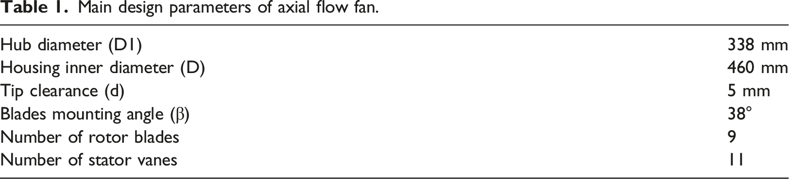
Figure 1(a) displays the physical model of the axial flow fan, while Figure 1(b) depicts the geometric model used in calculations, obtained through 3D scanning of the fan’s physical counterpart. Table1 provides a comprehensive overview of its principal structural parameters. Comprising rotors, stators, a hub, a motor, a baffle plate, and other associated components, the axial fan is equipped with pipes at its inlet and outlet to effectively suppress backflow from the outlet and ensure stable monitoring of flow and pressure throughout the experimental process. The diameter of the pipes, denoted as D, measures 6D for the inlet pipe and 4D for the outlet pipe.

Figure 1.

The model of the axial flow fan.

Table 1.

Main design parameters of axial flow fan.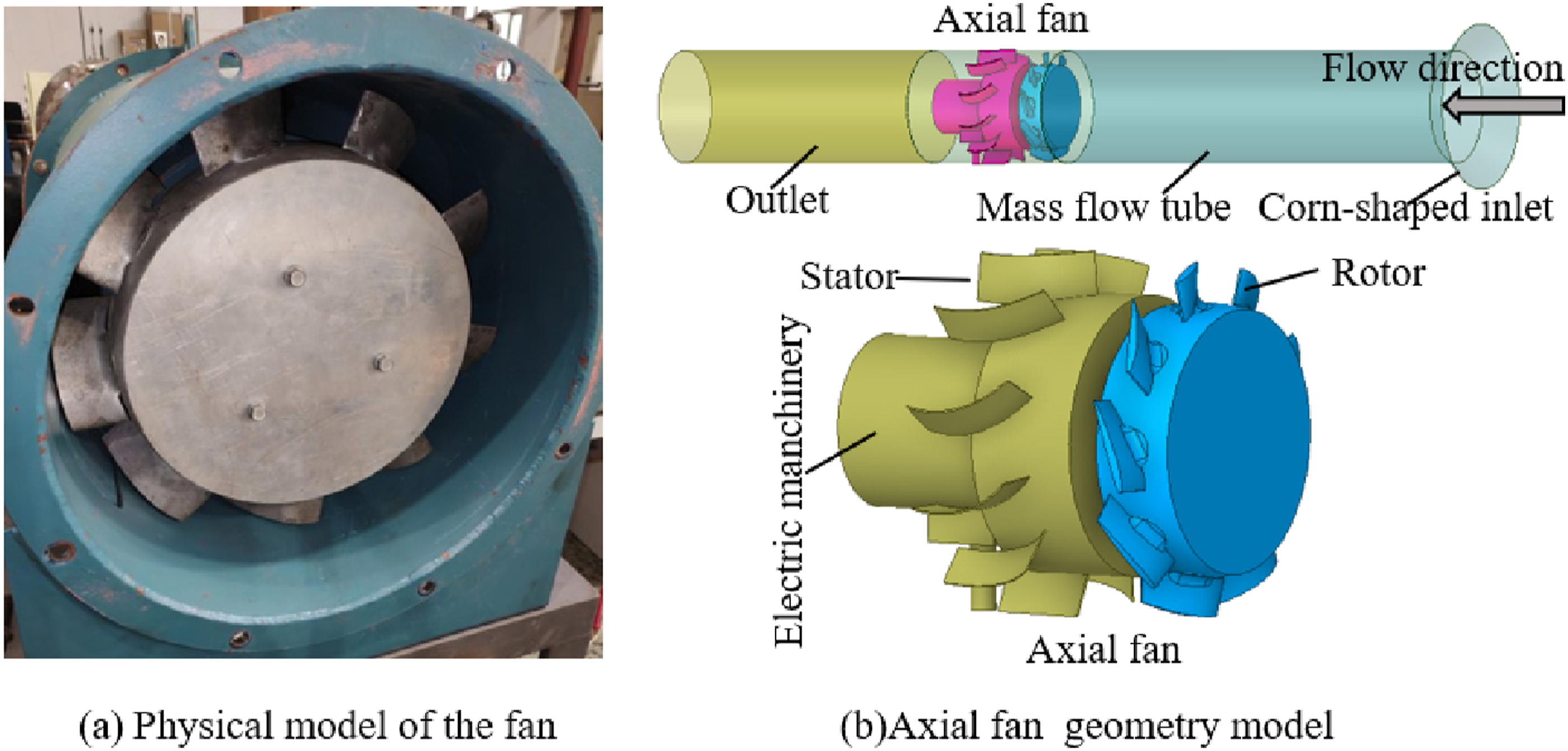

Hub diameter (D1)	338 mm
Housing inner diameter (D)	460 mm
Tip clearance (d)	5 mm
Blades mounting angle (β)	38°
Number of rotor blades	9
Number of stator vanes	11

Noise reduction models and principles

Noise reduction principle

During the operation of the axial fan, due to the work done by the rotor blades, the pressure difference between the PS and the suction surface (SS) causes the mainstream to flow to the SS through the TC to form the TLF, as shown by the gray arrow in Figure 2(b), and the TLF interacts with the mainstream to form the TLV. From the conclusions drawn in prior studies presented in the introduction and the subsequent analysis, it is the TLV that becomes the predominant vortex in the rotor wake and exerts an influence on the RSI (rotor-wake-stator interaction). The noise reduction model illustrated in Figure 2(b) was created through the perforation process from the LE to the PS. As illustrated in Figure 2(a), the pressure of LE is notably higher than that of PS and because of the pressure disparity, the mainstream gas can effortlessly enter the vent hole (indicated by blue arrows) and subsequently discharges from the PS (indicated by red arrows). The discharged gas acquires substantial kinetic energy and retains some of the gas that should flow towards the TC, directing it rearward (indicated by the black arrow). This process leads to the attenuation of the TLV, thus influencing the RSI and ultimately achieving the objective of noise reduction.

Figure 2.

Noise-reduction model and Noise-reduction schematic.

Innovation points

Indeed, previous studies on noise reduction through perforation have been conducted. For instance, Hu et al.³⁹ explored the reduction of noise by perforating both the LE and TE of the rotor blades. This approach aimed to mitigate noise by diminishing the SS separating vortices. Similarly, Yang et al.⁴⁰ investigated noise reduction through perforation near the tip of the blades. They achieved a 3 dB reduction in noise and analyzed that the improvement in shedding vortices from the TE of the blades was the underlying reason for this reduction. Furthermore, Chen et al.^41,42 conducted studies in which they perforated the trailing edges of the upstream rotor blades to achieve noise reduction.

The noise reduction model proposed in this paper offers distinct advantages over previous perforation models in the following ways:

(1) Targeted Vortex Reduction: While most existing perforation models focus on mitigating TE shedding vortices or SS separation vortices, the noise reduction model examined in this study specifically targets TLV. Indeed, in practice, it is commonly observed that the TLV exert the most significant influence on the aerodynamic noise of axial fans.

(2) Minimal Impact on Rotor Performance: The majority of previous noise reduction models that employ holes through PS to SS, which lead to some air to flow from the PS to the SS through the stomata and impact both the blade’s doing-work and the fan’s flow rate. The perforation model presented in this paper avoids penetrating the blades and has a relatively minor impact on the overall performance of the axial fan. Subsequent analysis will reveal the specific influence of the noise reduction model on the aerodynamic performance of the fan.

Noise reduction model structural parameters

Two noise-reduction blades, denoted as Blade A and Blade B, are assessed and their full details are given in Figure 3. They both have nine exit holes on the PS that are 1.2 mm in diameter and spaced 10 mm apart. The first exit hole is 25 mm from the LE and the last exit hole is 13 mm from the TE. The exit ducts form a 150° angle with the chord. Blade A has one entry hole that is 2.4 mm in diameter, and its axis is aligned with the medium arc of the cross-section. Blade B has two additional entry holes that are 2 mm in diameter. The ratio of the inlet area to the outlet area, denoted as S_in/S_out, is 0.44 and 1.06 for Blade A and Blade B, respectively.

Figure 3.

Original and Noise-reduction blade models and dimensions.

Numerical simulation of flow field

Mesh information

The numerical simulation of the flow field encompasses three distinct domains: the inlet domain, the rotor domain, and the outlet domain that includes the stators. The Poly-Hexcore mesh is generated using Fluent-Meshing. To ensure the accurate depiction of the flow structure within the TC, which plays a crucial role in capturing the vortex volume of the TLV during rotor motion,^43,44 it is essential to incorporate a sufficient number of grid layers in this region.^45,46 Therefore, refinement is applied to the rotor blades, stator vanes, and the wall at the TC. These specific areas are assigned a boundary layer mesh consisting of 10 layers, with the height of the first layer set at 0.06 mm. The detailed mesh configuration is illustrated in Figure 4. With the utilization of this flow simulation mesh, the Y+ value is maintained at less than 5 for the rotor blades and less than 2 for the stator vanes, as depicted in Figure 5.

Figure 4.

Mesh information of key areas.

Figure 5.

Y+ distribution clouds of rotor blades and stator vanes.

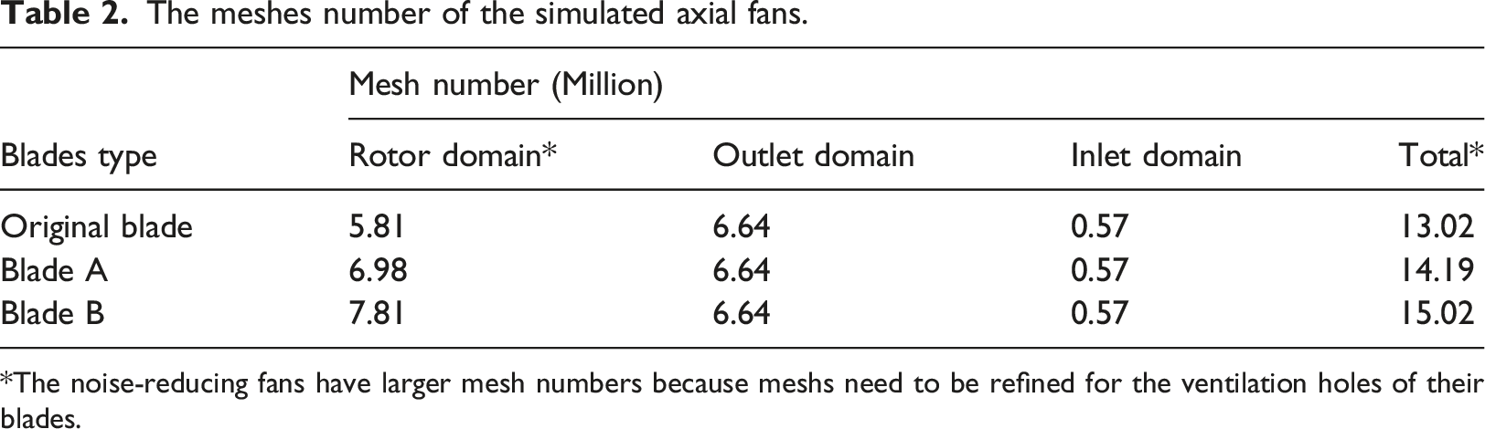
To examine the impact of mesh resolution on the calculation results, four sets of mesh with varying numbers (7.3, 9.4, 13.0, and 15.9 million) are generated for the original axial fan, as depicted in Figure 6. Among these options, the third scheme with a mesh number of 13.0 million is chosen for subsequent calculations due to its ability to maintain computational accuracy while requiring the least computational resources. Table 2 provides a summary of the mesh information employed for the simulated axial fans.

Figure 6.

Verification of mesh independence.

Table 2.

The meshes number of the simulated axial fans.

Blades type	Mesh number (Million)
Blades type	Rotor domain*	Outlet domain	Inlet domain	Total*
Original blade	5.81	6.64	0.57	13.02
Blade A	6.98	6.64	0.57	14.19
Blade B	7.81	6.64	0.57	15.02

*The noise-reducing fans have larger mesh numbers because meshs need to be refined for the ventilation holes of their blades.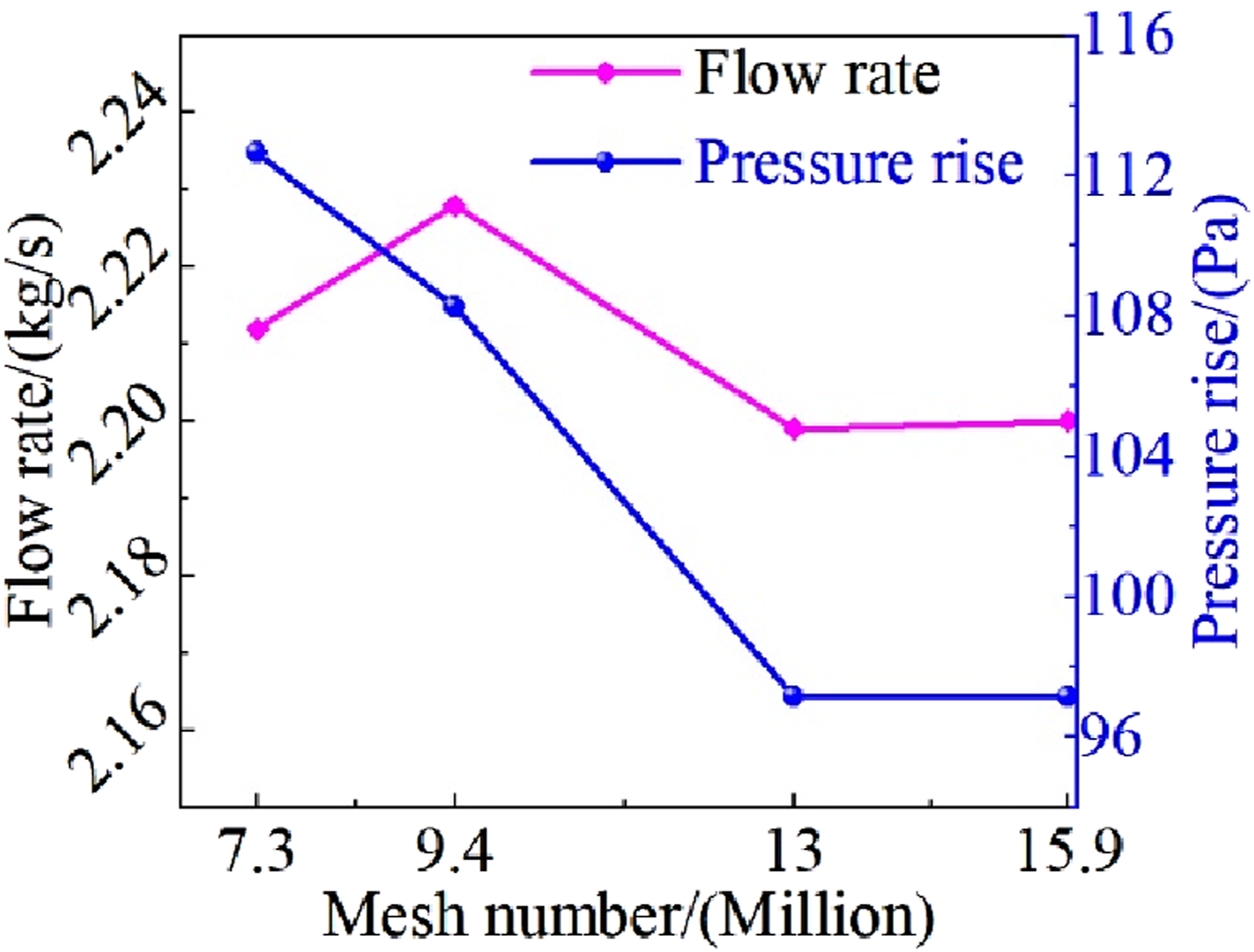

Boundary conditions

Given that the rated working condition of the existing experimental equipment is 2200rpm, this paper selects the 2200rpm working condition for analysis. The incoming Reynolds number is 2.97*10⁵, considering the inlet pipe diameter as the characteristic size. The incoming Mach number is 0.026, and the maximum Mach number in the pipe is 0.23. Since the maximum Mach number remains below 0.3, it would have been feasible to consider the medium as a constant density gas. Nevertheless, in this study, the fluid medium is treated as an ideal gas, and the energy equation is incorporated in the calculations to ensure better conformity of the working medium with the test conditions. The inlet boundary condition is defined by specifying the total pressure, while the outlet boundary condition is set to the static pressure. Within the rotating domain, both the rotor blades surface and the hub surface are treated as non-slip wall surfaces. Additionally, at the interface between the rotating and static domains, the surface is designated as the Interface, enabling efficient data interaction between these domains.

Solving methods

Within the fan, an intricate non-constant flow field emerges as a result of the interaction between the rotors and the stators. To numerically analyze this flow field, the k-w SST turbulence model is employed in the STARCCM + software. This turbulence model has high prediction accuracy for near-wall flow compared to other RANS turbulence models.^47–49 The pressure-velocity equations are solved using the SIMPLE algorithm, while the calculation of gradients adopts a cell-based least squares method. In the momentum equation and the turbulence scalar equation, a second-order upwind scheme is employed for the convection term, a central difference scheme is utilized for the diffusion term, and a second-order Euler implicit scheme is applied for the time term. The numerical calculation of flow field utilizes the steady-state calculation method to achieve convergence firstly. This approach provides initial data for unsteady-state simulations, thereby reducing the computation time required for unsteady-state simulations. For steady-state simulations, the Multiple Reference Frame (MRF) method is employed, while for unsteady-state simulations, the mesh motion method is utilized. The rotational speed of the fan is set at 2200 rpm. In the unsteady-state calculation, a time step of 7.5757 × 10⁻⁵ s is chosen, corresponding to a 1° movement of the rotor per time step. To ensure stability and accurate results, an initial rotation of the rotor is performed for three complete turns, equivalent to 360 × 3 time-steps. This initial rotation allows the monitoring points to exhibit stable and periodic fluctuations. Subsequently, the flow field data for the subsequent three turns is saved and used for the acoustic calculations that follow.

Acoustic calculation

Prediction theory of aeroacoustics

For a compressible gas, the acoustic analogy equation ⁵⁰ can be written as:

\frac{\partial^{2}}{\partial t^{2}} (ρ - ρ_{0}) - a_{0}^{2} \frac{\partial^{2}}{\partial x_{i} \partial x_{i}} (ρ - ρ_{0}) = \frac{\partial^{2} T_{ij}}{\partial x_{i} \partial x_{j}}

(1)

T_{ij} = ρ v_{i} v_{j} + ((p - p_{0}) - a_{0}^{2} (ρ - ρ_{0})) δ_{ij} - τ_{ij}

(2)

where ρ is the density, ρ₀ is the static density, v_i is the velocity vector, p is the pressure, a₀ is the stationary speed of sound, τ_ij is the viscous stress tensor, and T_ij is Lighthill’s tensor.

For a Stokes perfect gas in isentropic, high Reynolds number, and low Mach number flow, the Lighthill’s tensor can be approximated as⁵¹:

T_{ij} \approx ρ_{0} v_{i} v_{j}

(3)

By using ρ_a to replace ρ − ρ₀, equation (1) can be written as:

\frac{\partial^{2} ρ_{a}}{\partial t^{2}} - a_{0}^{2} \frac{\partial^{2} ρ_{a}}{\partial x_{i} \partial x_{i}} = \frac{\partial^{2} T_{ij}}{\partial x_{i} \partial x_{j}}

(4)

The integral formulation of Lighthill’s analogy, which is widely recognized as Curle’s analogy, was initially derived by Curle.⁵² In its integral form, the wave equation (Equation (1)) can be rewritten:

ρ - ρ_{0} = \frac{1}{4 π a_{0}^{2}} \int_{Ω} {[\frac{\partial^{2} T_{i j}}{\partial x_{i} \partial x_{j}} \frac{1}{r}]}_{t^{'}} d y + \frac{1}{4 π} \int_{Γ} {[\frac{1}{r} \frac{\partial}{\partial n} (ρ - ρ_{0}) + \frac{1}{r^{2}} \frac{\partial r}{\partial n} (ρ - ρ_{0}) + \frac{1}{a_{0} r} \frac{\partial r}{\partial n} \frac{\partial}{\partial t} (ρ - ρ_{0})]}_{t^{'}} d y

(5)

where Γ denotes the boundary of the acoustic domain, r = |x−y|, and the integrals’ arguments are evaluated at the retarded time t₀ = t − r/a₀. Starting from this equation, Curle transforms the right-hand side by integrating the volume integral by parts using Green’s theorem twice, and applies some transformations to the surface integral to obtain:

\begin{array}{l} ρ - ρ_{0} = \frac{1}{4 π a_{0}^{2}} \frac{\partial^{2}}{\partial x_{i} \partial x_{j}} \int_{Ω} {[\frac{T_{i j}}{r}]}_{t^{'}} d y + \frac{1}{4 π a_{0}^{2}} \int_{Γ} {[n_{i} \frac{1}{r} \frac{\partial}{\partial y_{j}} (T_{i j} + a_{0}^{2} (ρ - ρ_{0}) δ_{i j})]}_{t^{'}} d y \\ + \frac{1}{4 π a_{0}^{2}} \frac{\partial}{\partial x_{i}} \int_{Γ} {[n_{j} \frac{1}{r} (T_{i j} + a_{0}^{2} (ρ - ρ_{0}) δ_{i j})]}_{t^{'}} d y . \end{array}

(6)

Upon introducing the T_ij into equation (6) and subjecting it to a series of transformations, the following result is obtained:

\begin{array}{l} ρ - ρ_{0} = \frac{1}{4 π a_{0}^{2}} \frac{\partial^{2}}{\partial x_{i} \partial x_{j}} \int_{Ω} {[\frac{T_{i j}}{r}]}_{t^{'}} d y + \frac{1}{4 π a_{0}^{2}} \frac{\partial}{\partial x_{i}} \int_{Γ} {[n_{j} \frac{1}{r} (ρ v_{i} v_{j} + (p - p_{0}) δ_{i j} - τ_{i j})]}_{t^{'}} d y \\ - \frac{1}{4 π a_{0}^{2}} \int_{Γ} {[n_{i} \frac{1}{r} \frac{\partial}{\partial t} (ρ v_{i})]}_{t^{'}} d y . \end{array}

(7)

On the left-hand side of the equation, the fluctuation operator is depicted. Meanwhile, on the right-hand side of the equation, one can interpret the sound field as a combination of contributions from a volume distribution of quadrupoles and a surface distribution of dipoles and monopoles. For a detailed derivation of the integral form of Lighthill’s acoustic analogy equation, readers are referred to reference 53.

In addition to its integral form, the Lighthill acoustic analogy equation can be subject to variational differentiation as follows.

Equation (4) can be transformed to the frequency domain to give the Helmholtz equation:

- ω^{2} ρ_{a} - a_{0}^{2} \frac{\partial^{2} ρ_{a}}{\partial x_{i} \partial x_{i}} = \frac{\partial^{2} T_{ij}}{\partial x_{i} \partial x_{j}}

(8)

For compatibility with the formulation, a transformed potential was used:

ρ_{a} = - \frac{i ω ψ}{a_{0}^{2}}

(9)

Where

ψ

is velocity potential and

ω

is the angular frequency.

The alternative equation for the acoustic analogy in the frequency domain can be expressed as:

\frac{ω^{2}}{a_{0}^{2}} ψ + \frac{\partial^{2} ψ}{\partial x_{i} \partial x_{i}} = \frac{1}{i ω} \frac{\partial^{2} T_{ij}}{\partial x_{i} \partial x_{j}}

(10)

The first proposal of a variational formulation for Lighthill’s acoustic analogy was made by Oberai et al.^54,55 A strong variational differentiation of equation (10) can be obtained:

\int_{Ω} \frac{ω^{2}}{a_{0}^{2}} ψ δ ψ d Ω + \int_{Ω} \frac{\partial^{2} ψ}{\partial x_{i} \partial x_{i}} δ ψ d Ω = \int_{Ω} \frac{1}{i ω} \frac{\partial^{2} T_{i j}}{\partial x_{i} \partial x_{j}} δ ψ d Ω

(11)

where

δ ψ

is a test function and

Ω

is part of the computational domain. The spatial derivatives on the right-hand side of equation (11) can be partially integrated using Green’s theorem to obtain the weak variational form:

- \int_{Ω} \frac{ω^{2}}{ρ_{0} a_{0}^{2}} ψ δ ψ d Ω - \int_{Ω} \frac{1}{ρ_{0}} \frac{\partial ψ}{\partial x_{i}} \frac{\partial δ ψ}{\partial x_{i}} d Ω = S_{Ω} + S_{Γ}

(12)

S_{Ω} = \int_{Ω} \frac{i}{ρ_{0} ω} \frac{\partial δ ψ}{\partial x_{i}} \frac{\partial T_{ij}}{\partial x_{j}} d Ω

(13)

S_{Γ} = - \int_{Γ} \frac{δ ψ}{i ρ_{0} ω} \frac{\partial}{\partial x_{i}} (a_{0}^{2} ρ_{a} δ_{ij} + T_{ij}) n_{i} d Γ

(14)

In contrast to Curle’s integral form, the variational formulation of Lighthill’s acoustic analogy does not segregate the distinct contributions. Instead, the sound sources are categorized as volume sources and surface sources. In the above equation, S_Ω and S_Γ denote the contributions of the volume and surface sources, respectively, to the overall sound pressure. Specifically, in the context of a rotating machine, the stationary region within the machine is regarded as the volume source, while the surface of the rotor domain is considered the surface source.

Acoustic field calculation model

In accordance with the variational formulation of Lighthill’s acoustic analogy equation, the classification of sound sources originating from axial fans is conducted, segregating them into the distinct groupings of volume sources and surface sources. As shown in Figure 7, the Stator subdomain is taken as the volume source and the Interface is taken as the surface source. Positioned equidistantly between the rotor hub and the stator hub, the Interface is situated at a distance of 25 mm from the uppermost point of the rotor’s TE.

Figure 7.

Sound field calculation model.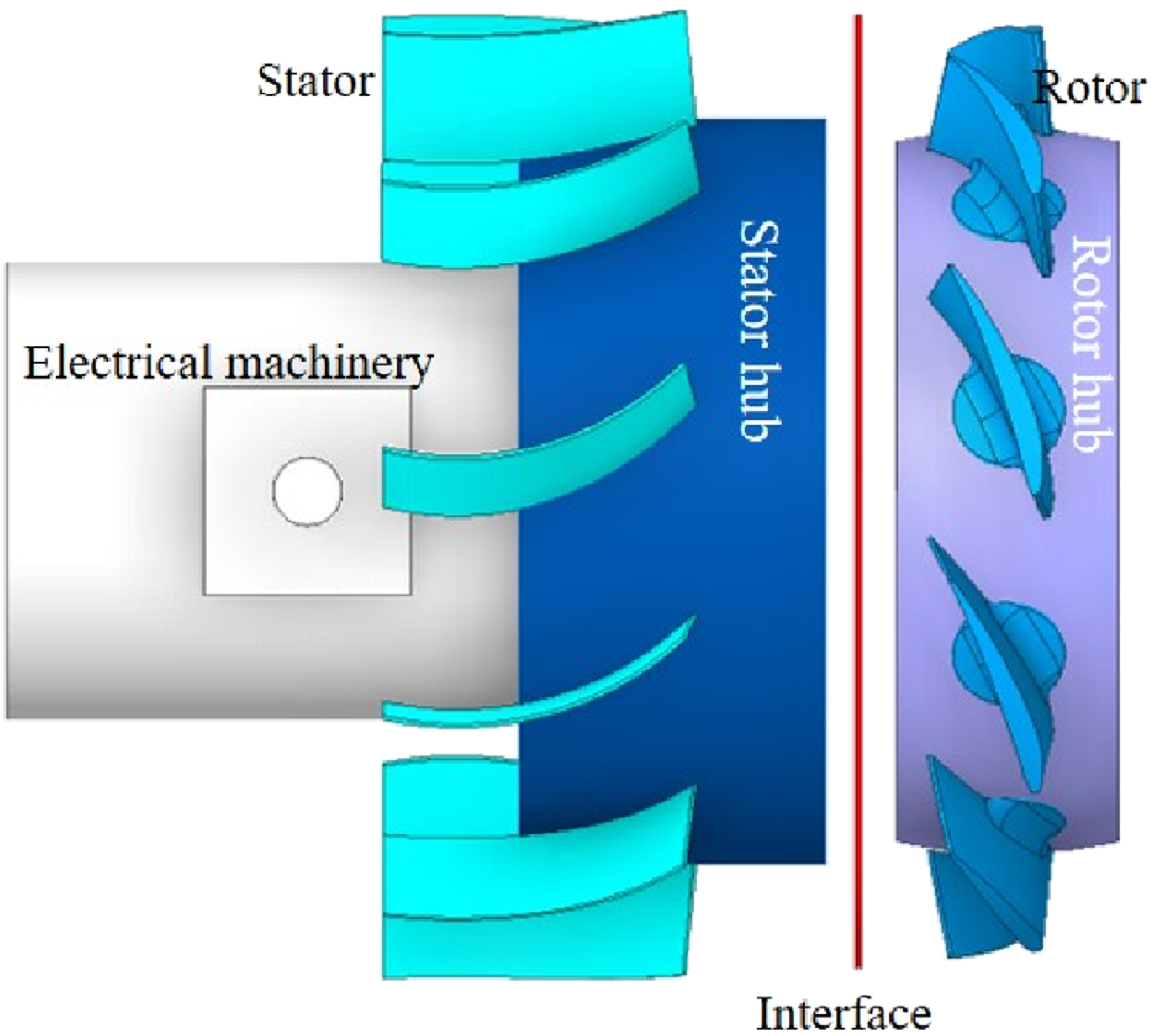

Acoustic computational domains and meshes

Illustrated in Figure 8, the computational domain for the acoustic field encompasses three three-dimensional regions: the stator domain, the rotor domain, and the inlet pipe. Additionally, the domain includes two two-dimensional representations denoting the interface and the inlet surface. Due to the non-recognition of the Poly-hexcore mesh within the ACTRAN software framework, the acoustic computational domain necessitates division into tetrahedral meshes.To ensure the accuracy of the acoustic calculation, it is necessary for each acoustic wavelength to encompass at least 6 cells, as specified in references 56,57. The maximum size of the acoustic calculation mesh is set at 14 mm, and for the frequency of 3000 Hz, the corresponding wavelength contains 8 cells, as shown in Figure 8.

Figure 8.

Acoustic computational domains and meshes.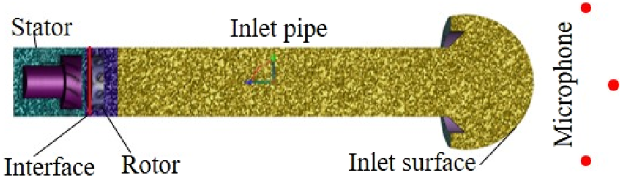

Acoustic calculation settings

The acoustic calculation commences with a well-defined specification of the frequency range to be analyzed. For rotating machinery, the frequency of tonal noise can be calculated based on the rotation speed of the turbine and the number of rotor blades as follows:

f = \frac{nzi}{60}

(15)

where n is the rotation speed of the fan, z is the number of rotor blades, i is the harmonic number (i = 1, 2, 3…), and f is BPF when i = 1. In this work, the fan rotation speed is 2200 rpm and there are 9 rotor blades. The BPF can be calculated from equation (15) as 330 Hz. Since in general the first three harmonics of BPF contribute the most to the OSPL in rotating machinery, the highest frequency of the acoustic calculation is set to 3000 Hz to meet the prediction requirements.

Next, the Stator domain, Rotor domain, and Inlet pipe are defined as finite element bodies. Meanwhile, the Inlet surface is designated as an infinite element surface. The media for both the finite element bodies and infinite element surface are set as air, with a sound velocity of 340 m/s and a density of 1.225 kg/m³, which indicates that the noise propagates in the pipe air and radiates through the infinite element surface to the atmosphere.

In the process of setting boundary conditions, the Stator domain is designated as the Lighthill Volume, while the Interface is set as the Lighthill surface. Subsequently, the time-domain source information at the corresponding location in the flow field data is mapped to the Lighthill Volume and Lighthill surface and solved using the MUMPS solver.⁵⁸ The time domain sound source is converted to frequency domain sound source by iCFD, and then the propagation of the sound source inside the pipe and the radiation outside the pipe through the infinite element face are calculated. Finally, three Microphones are set up as monitoring points to receive acoustic signals. Figure 9 shows the acoustic calculation process.⁵⁹

Figure 9.

Flow chart of noise prediction based on CFD results.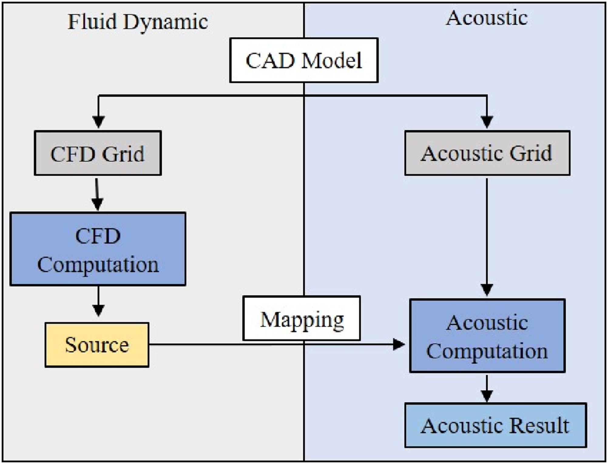

Pipe sound propagation analysis

Among the various types of aerodynamic noises associated with rotating machinery, our primary focus lies in tonal noise. Tonal noise predominantly originates from the RSI, which is analyzed in the subsequent section. Impeller duct noise propagates in modal form due to the presence of duct walls. Let the pipe modes be (m, n), m is the circumferential mode and n is the radial mode. From the Tyler-Sofrin² modal theory, the dominant mode of each order of harmonics is $m = h B - k V; k = 0, 1, 2 \dots$ where m is the circumferential mode, h is the number of harmonics, B is the number of rotor blades, V is the number of stator vanes, and k is an arbitrary integer. Meanwhile, the cut-off frequency of each order mode can be found from:

f_{mn} = \sqrt{1 - M^{2}} \frac{α_{mn} C}{2 π a}

(16)

where M is the Mach number of the pipeline fluid, the inlet flow velocity is about 12 m/s,

α_{mn}

is the nth zero point of the derivative of the m-th order Bessel function of the annular pipe, c is the speed of sound, and a is the inlet diameter.

Table 3 presents the dominant modes of each order harmonic along with their respective cut-off frequencies. An examination of Table 3 reveals that the harmonic frequencies for each order remain below the corresponding dominant mode’s cut-off frequency, thereby rendering the propagation of these modes within the pipe infeasible. Figure 10 shows the sound pressure cloud of the dominant mode in the pipe corresponding to the first three harmonics. From the figure, it can be seen that the modes in the table attenuate very quickly and can’t be propagated in the pipe, which is consistent with the results of the theoretical analysis.

Table 3.

Interaction modes and cut-off frequencies.

	Frequency/Hz	k	m	Mode	fcut-off/Hz
1BPF(h = 1)	330	1	−2	(-2,0)	718
2BPF(h = 2)	660	2	−4	(-4,0)	988
3BPF(h = 3)	990	2	5	(5.0)	1509

Figure 10.

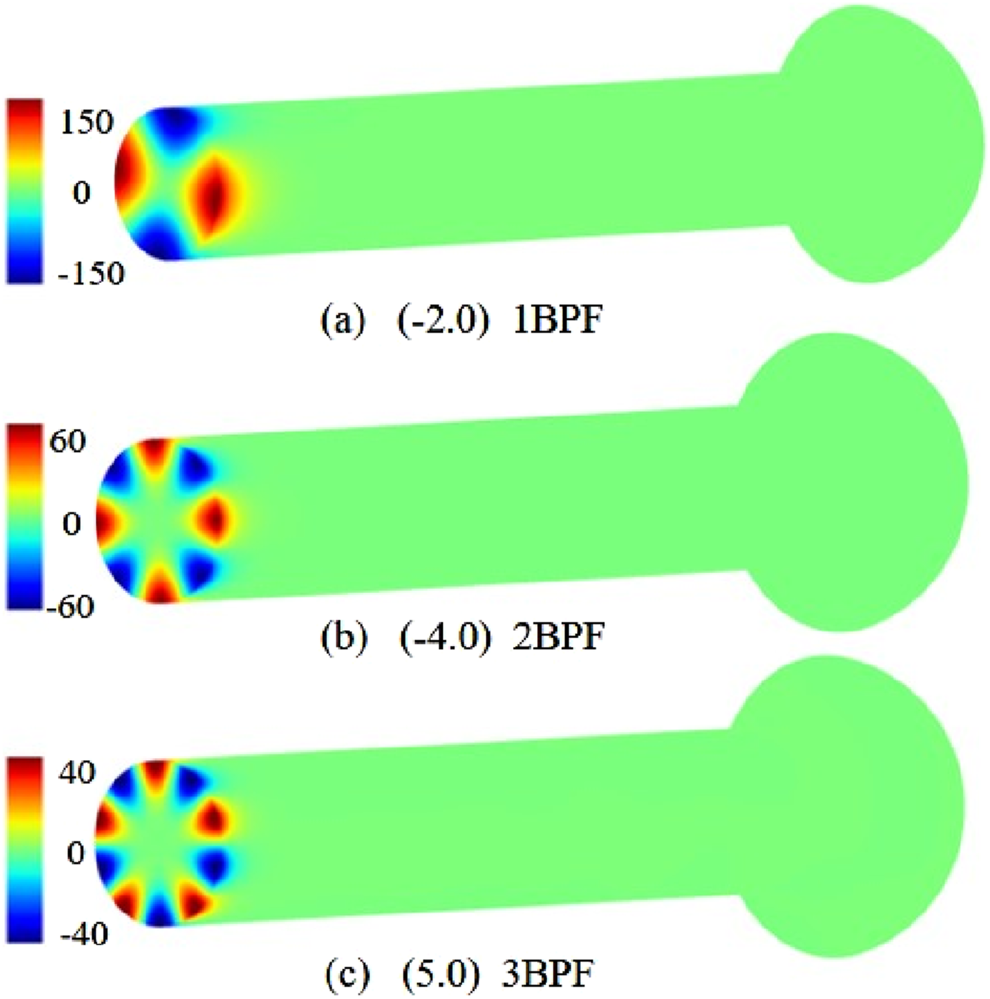
Blade passing frequency and harmonic mode propagation.

Experimental verification

Aerodynamic performance experiment

The investigation of the aerodynamic performance and aerodynamic noise of the axial flow fan was carried out utilizing the experimental rig depicted in Figure 11. The aerodynamic performance was assessed in accordance with the Chinese national standard GB/T 1236-2000.⁶⁰ To achieve a rotational speed of 2200 rpm, the TCVX axial flow fan was adjusted using a three-phase variable-frequency drive. The mass flow rate of the fan was measured using a hot-wire anemometer located at position A1. Since the hot-wire anemometer readings fluctuated during the experiment, more than 20 sets of data were read for averaging to reduce the test error. Furthermore, the average pressure at section B was recorded using a U-tube manometer. The U-tube manometer had a main hose connected to four branches, each linking to one of the monitoring points (B1, B2, B3, and B4). The resolution of the U-tube manometer was set at 10 Pa.

Figure 11.

The schematic and the picture of the test bench.

Aerodynamic noise experiment

The acoustic measurements were conducted following the requirements of GB/T 2888-1991.⁶¹ For acoustic measurements, three B&K4189 acoustic microphones were positioned at a distance of 1 m from the center of the fan inlet. One microphone was placed on the inlet axis, while the other two were positioned at a 45° angle to the axis. Due to the substantial impact of motor noise on the outlet noise, it was challenging to obtain accurate aerodynamic noise results near the outlet. Therefore, the microphones were strategically placed near the inlet. Prior to the sound field measurements, background noise was first measured, defined as the sound pressure recorded by the three microphones when the inverter was operating and the fan was not started. Then, the fan is driven to 2200 rpm by the inverter, and the sound pressure information is recorded when the hot-wire anemometer and manometer readings are stable. Acoustics data acquisition was performed using the PULSE system with a sampling time of 30 s. The acquired data was subsequently processed using the Reflex system to generate a sound pressure frequency spectrum curve with a resolution of 2 Hz.

Results and analysis

Experimental verification of numerical simulation results

In both the mass flow rate and the pressure difference, a relatively small difference is observed between the simulation and experimental results, as depicted in Table 4.

Table 4.

Comparison of experimental and simulation results.

	Experiment	Simulation	Difference (%)
Flow rate (kg/s)	2.37	2.24	5.49
Pressure difference* (Pa)	100	92.18	7.82

*The difference between the atmospheric pressure and the static pressure at the monitoring points.

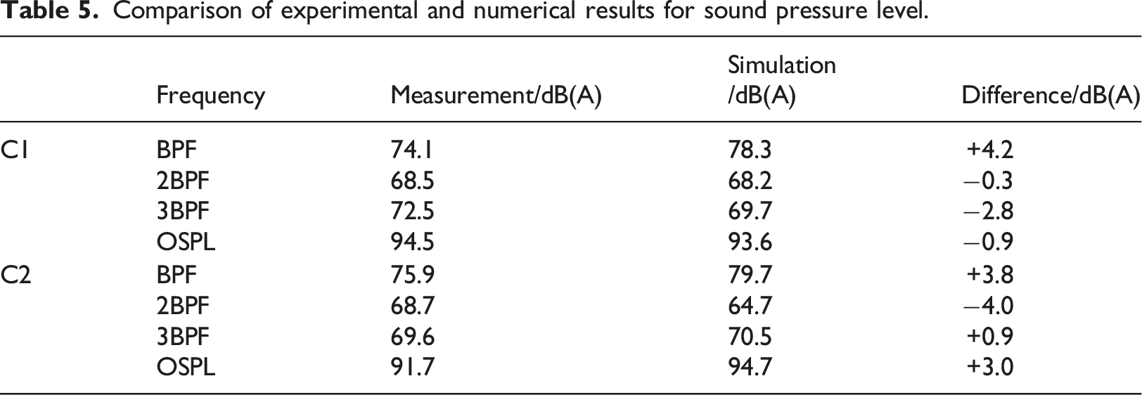
From the sound pressure spectrum curve, it is evident that the background noise during the acoustic test is substantially lower in magnitude compared to the fan noise. This background noise has minimal impact on the accuracy of the measurements. For the measured fan noise, a frequency resolution of 2 Hz is employed, while in numerical simulation, a resolution of 12 Hz is adopted due to simulation time constraints. The simulation results yield an A-weighted SPL spectral curve, revealing a distinctive tonal noise characteristic. Notably, the BPF exhibits the highest sound pressure value, whereas the sound pressure at 2BPF is lower than that at 3BPF. Furthermore, the magnitudes of the tonal noise at the first three harmonics align closely with the experimental findings, as depicted in Figure 12. The difference in OSPL at the two monitoring points are 0.9 dB(A) and 3.0 dB(A), respectively, as outlined in Table5. Consequently, the proposed numerical simulation method successfully demonstrates its capacity to accurately predict the aerodynamic noise generated by the axial fan. For the noise calculation pertaining to the noise reduction model, monitoring point C1 is chosen, given its lower OSPL difference.

Figure 12.

Comparison of the simulated and experimental sound pressure curves at the monitoring point C1 and C2.

Table 5.

Comparison of experimental and numerical results for sound pressure level.

	Frequency	Measurement/dB(A)	Simulation/dB(A)	Difference/dB(A)
C1	BPF	74.1	78.3	+4.2
	2BPF	68.5	68.2	−0.3
	3BPF	72.5	69.7	−2.8
	OSPL	94.5	93.6	−0.9
C2	BPF	75.9	79.7	+3.8
	2BPF	68.7	64.7	−4.0
	3BPF	69.6	70.5	+0.9
	OSPL	91.7	94.7	+3.0

Analysis of the flow field

The accurate capture of vortices within the fan runners is of utmost importance for enhancing the precision of noise prediction, given their significant influence on aerodynamic noise. The vortex distribution cloud at various span sections of the fan is illustrated in Figure 13. At the 98% span section, the TLV is generated near the LE at 1/3 chord length and undergoes a defined motion towards the SS of the stator vanes, thereby instigating RSI. On the section aligned with the axis of the noise-reduction holes, the TLV emerges near the TE at 1/3 chord length and manifests two vortex cores. In the case of the original blade, these two vortex cores are in closer proximity, with the core at the TLV exhibiting a larger volume. The TLV assumes a pivotal role in aerodynamic noise generation, predominantly due to its significantly larger volume in comparison to the TE shedding vortex. In contrast, Blade A and Blade B exhibit substantially lower vortex volumes for the TLV when compared to the original blade (as indicated by the red circle). Although a notable vortex presence is observed within the noise-reduction holes, it does not propagate beyond the rotor blade’s outer region and contributes minimally to far-field noise (as highlighted by the black circle).

Figure 13.

The Q criterion vortex contour of the axial fan with (O) the original blade, (a) Blade A, and (b) Blade B (*In the following analysis, these three types of blades are represented by O, A, and B in the figure or table).

In Figure 14, the flow line of the original blade and the distribution of vortex volume for the three blades are presented. The distribution of the vortex volume in the transient field and the mean field within the region indicated by the red circle is noticeably larger for the original blade. The inner wall of the duct guides the airflow, as depicted by the black arrow, from one rotor to the SS of the subsequent rotor, owing to the compression exerted by the rotor. The pressure difference between the PS and the SS of the rotor prompts a portion of the airflow near the PS to traverse the TC and reach the SS, as indicated by the purple arrow. At the SS of the rotor blades, the airflow paths represented by the black and purple arrows intersect, resulting in the formation of the TLV.

Figure 14.

Vorticity cloud at 80% chord length for the axial fan.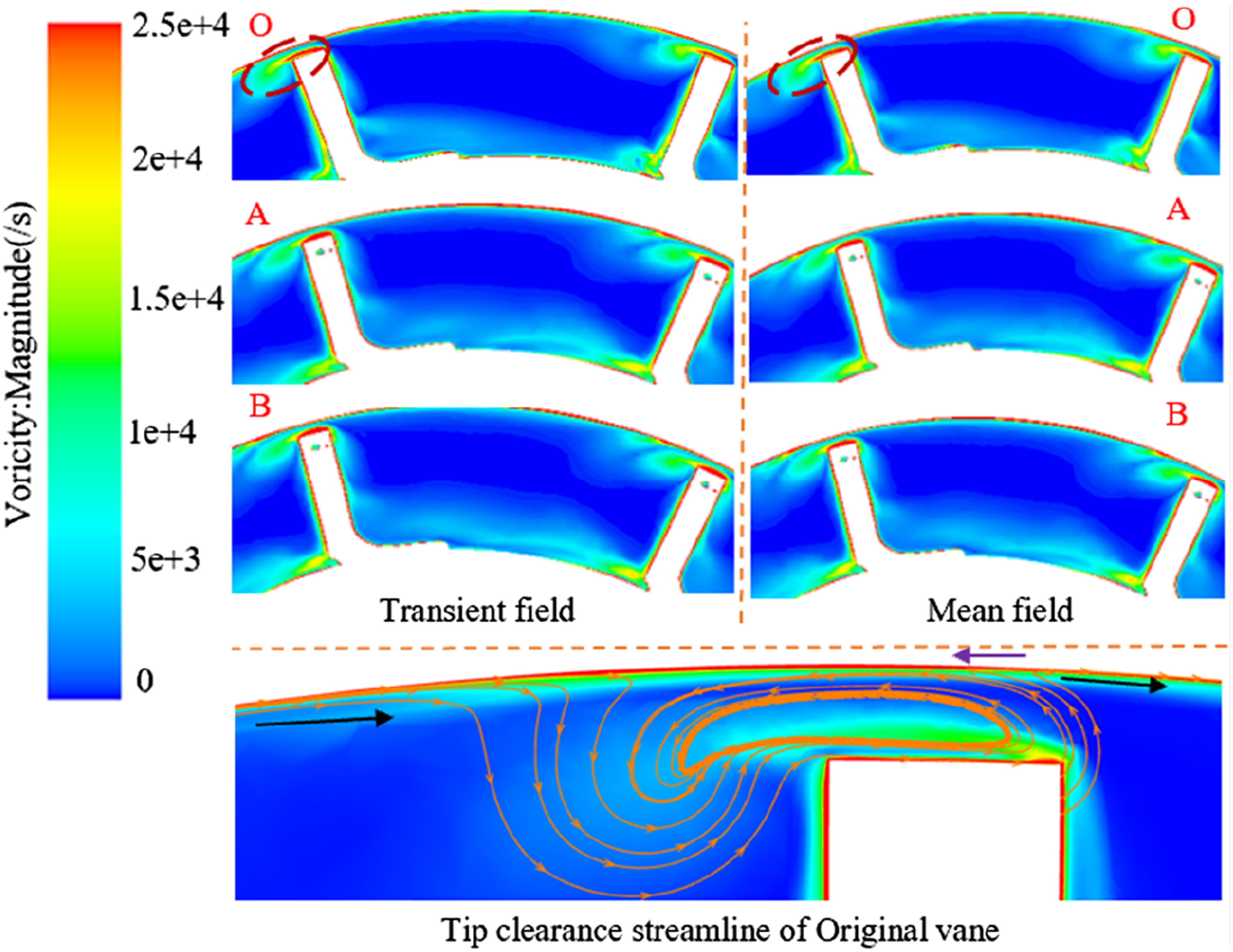

The size of the vortex can be effectively assessed by examining the entropy distribution at the TC. Two types of vortices, namely the TLV (black circle) and the interaction vortex (red circle), are present near the SS of the rotor blades. The interaction vortex arises from the interaction between the main stream and the TLV, rotating in the opposite direction to the TLV. Figure 15 illustrates seven equidistantly distributed sections, ranging from Surface 1 at the LE to Surface 7 located at 1/30 chord length from TE. The interaction vortex and TLV initiate near the LE and exhibit a distinct progression until they eventually merge. Notably, on Surface 5, the original blade demonstrates the onset of vortex merging, while Blade A and Blade B maintain separate vortices due to their attenuated characteristics. Blade A and Blade B effectively reduce the volume of the channel vortex, as indicated by the yellow circle.

Figure 15.

Entropy distribution cloud of the rotor domain for the axial fan.

The tonal noise in axial fans primarily originates from the RSI. The intensity of the sound source can be effectively assessed by the rate of pressure change. Within the fan, the LE of the rotor blades and the LE of the stator vanes SS serve as two significant noise sources (Figure 16). The presence of noise-reduction holes notably diminishes the intensity of the noise source at the LE of the stator vanes SS, and this reduction is more pronounced when Sin/Sout is larger. The airflow entering the inlet holes on the LE of the rotor blades induces substantial pressure fluctuations. In contrast, the noise-reduction blades exhibit significantly reduced pressure fluctuations at the remaining sections of the rotor blades LE.

Figure 16.

Blade pressure fluctuation cloud for the axial fan.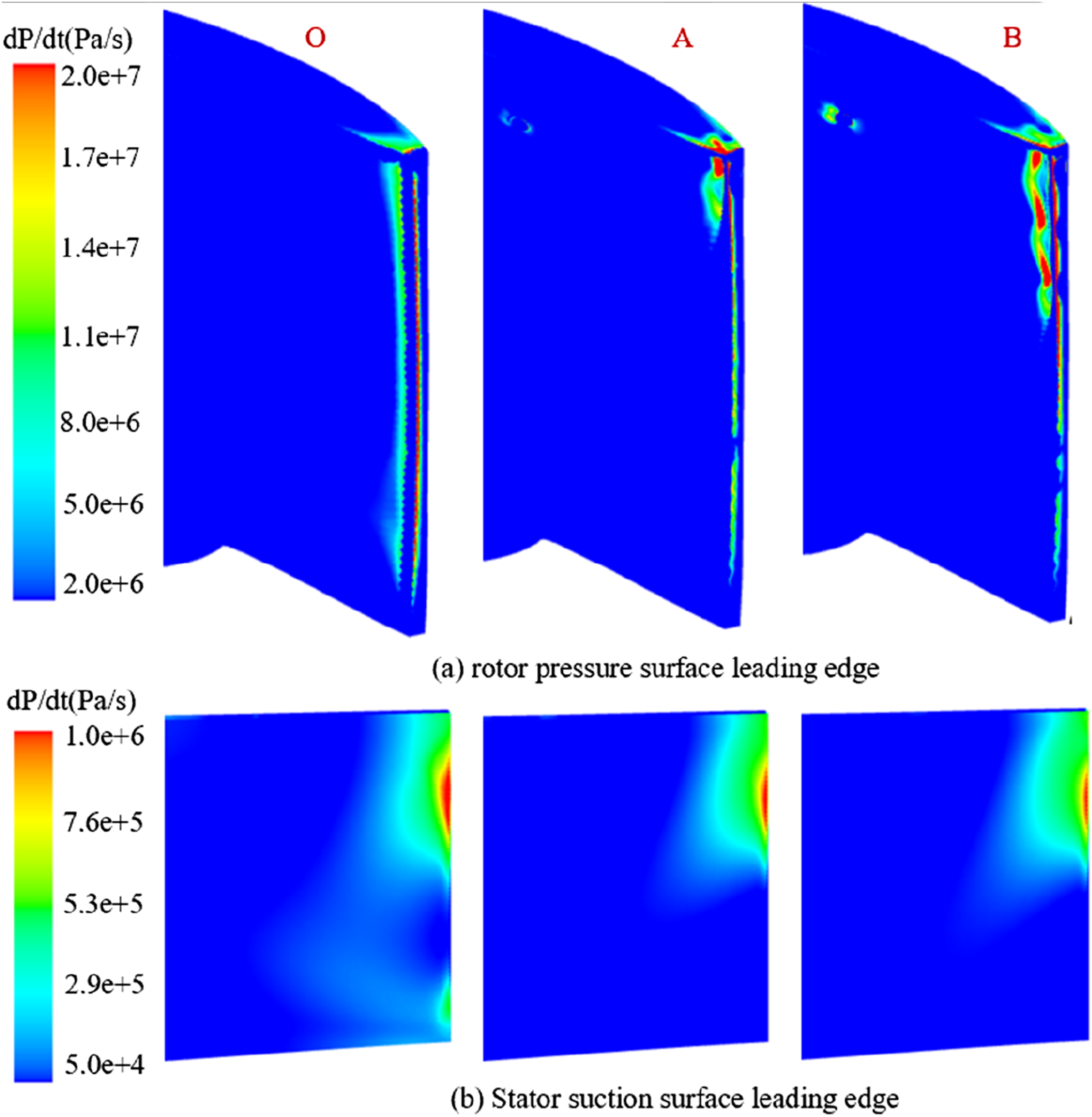

Acoustic field analysis

The sound pressure spectrum curves, obtained from the numerical simulation, are presented in Figure 17. Notably, all fans exhibit distinct tonal characteristics in the far-field noise, and the aerodynamic noise is effectively reduced by the modified blades. Blade A and Blade B achieve reductions of 3.3 dB(A) and 3.9 dB(A), respectively, in terms of the OSPL. The most significant noise reduction occurs at BPF, with reductions of 15.0 dB(A) and 17.9 dB(A) for Blade A and Blade B, respectively. However, it should be noted that the noise-reduction blades slightly increase the noise levels at 2BPF and 3BPF, as indicated in Table 6.

Figure 17.

Sound spectrum curve at monitoring point C1 for the three axial fans.

Table 6.

Comparison of the sound pressure level of three fans.

Blade	BPF/dB(A)	2BPF/dB(A)	3BPF/dB(A)	OSPL/dB(A)
O	78.3	68.2	69.7	93.6
A	63.3 (−15.0)	70.7 (+2.5)	70.3 (+0.6)	90.3 (−3.3)
B	60.4 (−17. 9)	70.3 (+2.1)	70.0 (+0.3)	89.7 (−3.9)

The performance parameters of the three blades are presented in Table 7. It is observed that the utilization of the noise-reduction blades leads to a slight increase in the flow rate and pressure rise. However, the most significant impact is observed in the static efficiency of the turbine, which is reduced by 0.5% and 0.26% with blade A and blade B, respectively. The pressure rise is the difference between the total outlet pressure and the total inlet pressure (P_rise = P_total,out−P_total,in) and static efficiency (η) is defined as:

η = \frac{Δ PQ}{T Ω}

(17)

where ΔP is the total pressure rise, T is the torque of the fan, Q is the volume flow rate, Ω is the fan rotational speed.

Table 7.

Aerodynamic performance of the three fans.

Blade	Flow rate (m³/s)	Pressure rise (Pa)	Efficiency (%)
O	1.86	92.8	75.26
A	1.88	95.4	74.76
B	1.88	93.0	75.00

The distribution of sound pressure at Lighthill surface is depicted in Figure 18. Significantly lower sound source intensity is observed for fans equipped with noise-reduction blades compared to the original fan at BPF. Conversely, noise-reduction blades have greater noise levels at the 2BPF and 3BPF. However, the maximum sound source intensity is observed at the BPF, as indicated by the scale on the cloud map. The findings presented herein are consistent with those reported in Table 6, further affirming substantial noise reduction at the BPF while exhibiting a moderate increase in noise at the second and third harmonic frequencies.

Figure 18.

Sound pressure cloud map from blade passing frequency to 3BPF at Lighthill surface.

To further explore the impact of noise-reduction blades on RSI, the pressure information from the stator surface is extracted for three revolutions and subjected to Fast Fourier Transform (FFT) calculations. The sound power density of the stator vanes at various harmonics is illustrated in Figure 19. The sound source density at the BPF surpasses that at 2BPF and 3BPF. Notably, at the BPF, the maximum sound source is observed near the upper region of the stator vanes, with the noise-reduction blades exhibiting smaller sound power density on LE of the stator vanes SS compared to the original blades. Conversely, at 2BPF and 3BPF, the noise-reduction blades display slightly higher sound source intensity relative to the original blades, yet the sound power density remains significantly lower than that at the BPF. Consequently, the dominant role of noise reduction at the BPF persists.

Figure 19.

Sound source intensity at the stator vanes suction surface leading edge.

Based on the aforementioned analysis, the noise reduction model outlined in this paper demonstrates efficacy in mitigating the aerodynamic noise emitted by the fan. However, the model does present certain limitations. Primarily, perforating from LE to PS has certain difficulties. Additionally, the small aperture of the noise reduction hole poses a risk of blockage over time, particularly when deployed in environments with high dust levels, potentially diminishing the effectiveness of the aperture.

Conclusions

In this study, the prediction of aerodynamic noise in an axial fan is achieved through the integration of STARCCM + fluid numerical simulation and ACTRAN acoustic calculation. The numerical predictions exhibit excellent agreement with the experimental results, thereby validating the effectiveness and accuracy of the employed prediction method. Notably, the accuracy of SPL estimation for the first three harmonics and the OSPL prediction is notably improved.

Given the large TC size of the investigated fan (with a TC size-to-blade height ratio of 8.2%), the vortex volume of the TLV is larger than that of the other vortices. The generation of TLV occurs primarily at the upper region of the blades near LE, subsequently propagating in a specific direction towards the stator region and impacts the LE of the stator vanes, causing significant RSI.

The primary noise source of the axial fan is located at the LE of the rotor blades and the LE of the stator vanes SS. Through the implementation of noise-reduction blades, the TLV is reduced, and the effects of RSI are weakened. As a result, the noise source at the LE of the stator vanes SS is reduced, leading to a significant decrease in SPL at BPF and OSPL within 3000 Hz. Besides, the noise reduction model proposed in this paper does not significantly affect the aerodynamic performance of the axial fan while realizing noise reduction.

A better noise reduction effect is observed when the ratio of the inlet area to the outlet area (S_in/S_out) is larger. When S_in/S_out is 1.06, the OSPL of the axial fan can be reduced by 3.9 dB(A). The noise-reduction blades exhibit the most effective reduction of noise at BPF, resulting in a decrease of 15.0 dB(A) and 17.9 dB(A) in SPL at BPF when S_in/S_out is 0.44 and 1.06, respectively.

Footnotes

Declaration of conflicting interests

The author(s) declared no potential conflicts of interest with respect to the research, authorship, and/or publication of this article.

Funding

The author(s) disclosed receipt of the following financial support for the research, authorship, and/or publication of this article: This work was supported by Fundamental Research Funds for the Central Universities (3072022TS0307).

ORCID iD

Guanghui Yang

References

Chai

Sun

Chang

, et al. Noise characteristics of automobile cooling fan based on circumferential mode analysis[J]. J Eng Gas Turbines Power 2021; 143(12): 121003.

Tyler

Sofrin

. Axial flow compressor noise studies[R]. SAE Technical Paper, 1962.

Foulquié

Khelladi

Deligant

, et al. Numerical assessment of fan blades screen effect on fan/OGV interaction tonal noise[J]. J Sound Vib 2020; 481: 115428.

Suzuki

Spalart

Shur

, et al. Unsteady simulations of a fan/outlet-guide-vane system: tone–noise computation[J]. AIAA J 2018; 56(9): 3558–3569.

Soulat

Kernemp

Sanjose

, et al. Numerical assessment of the tonal noise of Counter-Rotating Open Rotors at approach[J]. Int J Aeroacoustics 2016; 15(1–2): 23–40.

Hirono

Robertson

Torija Martinez

. Acoustic and psychoacoustic characterisation of small-scale contra-rotating propellers[J]. J Sound Vib 2024; 569: 117971.

Canepa

Cattanei

Zecchin

. Effect of the rotor–stator gap variation on the tonal noise generated by axial-flow fans[J]. Appl Acoust 2015; 94: 29–38.

Han

Zhang

, et al. Stator modification methods for diagonal flow fans to achieve noise reduction of rotor-stator interaction[J]. J Mech Sci Technol 2022; 36(2): 785–796.

Cooper

Peake

. Upstream-radiated rotor–stator interaction noise in mean swirling flow[J]. J Fluid Mech 2005; 523: 219–250.

10.

Crigler

Copeland

. Noise studies of inlet-guide-vane-rotor interaction of a single-stage axial-flow compressor[J] national aero-nautics and space administration, 1965. Washington, DC, Technical Note No. NASATN D-2962.

11.

Pan

Peng

, et al. Blade force model for calculating the axial noise of fans with unevenly spaced blades[J]. Appl Acoust 2019; 146: 429–436.

12.

Peng

Ouyang

, et al. Tonal noise control of cooling fan module by using modulation principles on both rotor and stator[C]//Turbo Expo: Power for Land, Sea, and Air. American Society of Mechanical Engineers, 2018, 50985: V001T09A007.

13.

Peng

Tian

, et al. Discrete noise control of cooling fan module: stator and rotor interaction[J]. Appl Acoust 2020; 165: 107308.

14.

Krömer

Czwielong

Becker

. Experimental investigation of the sound emission of skewed axial fans with leading-edge serrations[J]. AIAA J 2019; 57(12): 5182–5196.

15.

Park

Lee

. Tonal and broadband noise attenuation of an axial flow fan with forward and backward swept blades[J]. Appl Acoust 2022; 195: 108837.

16.

Tong

Qiao

, et al. On the study of wavy leading-edge vanes to achieve low fan interaction noise[J]. J Sound Vib 2018; 419: 200–226.

17.

Volkmer

Kaufmann

Carolus

. Mitigation of the aerodynamic noise of small axial wind turbines-methods and experimental validation[J]. J Sound Vib 2021; 500: 116027.

18.

Lyu

Azarpeyvand

. On the noise prediction for serrated leading edges[J]. J Fluid Mech 2017; 826: 205–234.

19.

Avallone

Pröbsting

Ragni

. Three-dimensional flow field over a trailing-edge serration and implications on broadband noise[J]. Phys Fluids. 2016; 28(11). doi:10.1063/1.4966633

20.

Liu

Zang

Azarpeyvand

. Wake-aerofoil interaction noise control with trailing-edge serrations[J]. Exp Therm Fluid Sci 2022; 130: 110510.

21.

Barakat

BeiBei

. Prediction of aerodynamic noise in axial fan using serration edge blades[J]. International Journal of Fluid Machinery and Systems 2020; 13(3): 570–582.

22.

Biedermann

Czeckay

Hintzen

, et al. Applicability of aeroacoustic scaling laws of leading-edge serrations for rotating applications[C]//Acoustics. MDPI 2020; 2(3): 579–594.

23.

Paruchuri

Narayanan

Joseph

, et al. Leading-edge serration geometries for significantly enhanced leading edge noise reductions[C]. In: 22nd AIAA/CEAS Aeroacoustics Conference, 2016, p. 2736.

24.

Chaitanya

Joseph

Ayton

. Leading-edge profiles for the reduction of airfoil interaction noise[J]. AIAA J 2020; 58(3): 1118–1129.

25.

Moghadam

SMA

Meinke

Schröder

. Analysis of tip-leakage flow in an axial fan at varying tip-gap sizes and operating conditions[J]. Comput Fluid 2019; 183: 107–129.

26.

Magne

Moreau

Berry

. Subharmonic tonal noise from backflow vortices radiated by a low-speed ring fan in uniform inlet flow[J]. J Acoust Soc Am 2015; 137(1): 228–237.

27.

Moreau

Sanjose

. Sub-harmonic broadband humps and tip noise in low-speed ring fans[J]. J Acoust Soc Am 2016; 139(1): 118–127.

28.

Fukano

Jang

C-M

. Tip clearance noise of axial flow fans operating at design and off-design condition[J]. J Sound Vib 2004; 275(3-5): 1027–1050.

29.

Luo

Chu

Zhang

. Tip leakage flow and aeroacoustics analysis of a low-speed axial fan[J]. Aero Sci Technol 2020; 98: 105700.

30.

Vemuri

Liu

Zang

, et al. On the use of leading-edge serrations for noise control in a tandem airfoil configuration[J]. Phys Fluids 2020; 32(7): 077102.

31.

Longhouse

. Control of tip-vortex noise of axial flow fans by rotating shrouds [J]. J Sound Vib 1978; 58: 201–214.

32.

Magne

Sanjosé

Moreau

, et al. Aeroacoustic prediction of the tonal noise radiated by a ring fan in uniform inlet flow[C]. In: 18th AIAA/CEAS Aeroacoustics Conference (33rd AIAA Aeroacoustics Conference), 2012, p. 2122.

33.

Magne

Moreau

Berry

. Subharmonic tonal noise from backflow vortices radiated by a low-speed ring fan in uniform inlet flow[J]. J Acoust Soc Am 2015; 137(1): 228–237.

34.

Moreau

Sanjose

. Sub-harmonic broadband humps and tip noise in low-speed ring fans[J]. J Acoust Soc Am 2016; 139(1): 118–127.

35.

Canepa

Cattanei

Zecchin

, et al. An experimental investigation on the tip leakage noise in axial-flow fans with rotating shroud[J]. J Sound Vib 2016; 375: 115–131.

36.

Tian

Liu

Wang

, et al. Effects of bionic blades inspired by the butterfly wing on the aerodynamic performance and noise of the axial flow fan used in air conditioner[J]. Int J Refrig 2022; 140: 17–28.

37.

Jung

Joo

. Effect of tip clearance, winglets, and shroud height on the tip leakage in axial flow fans[J]. Int J Refrig 2018; 93: 195–204.

38.

Lim

Jung

Jeon

, et al. Investigation study on the flow-induced noise by winglet and shroud shape of an axial flow fan at an outdoor unit of air conditioner[J]. J Mech Sci Technol 2020; 34: 2845–2853.

39.

Wang

, et al. Effects of perforation number of blade on aerodynamic performance of dual-rotor small axial flow fans[J]. J Therm Sci 2015; 24(2): 123–130.

40.

Yang

Wen

, et al. Numerical simulation and experimental research on the aerodynamic performance of large marine axial flow fan with a perforated blade[J]. J Low Freq Noise Vib Act Control 2018; 37(3): 410–421.

41.

Wang

Huang

. Passive noise reduction for a contra-rotating fan[C]//Turbo Expo: Power for Land, Sea, and Air. American Society of Mechanical Engineers, 2014, 45578: V01AT10A011.

42.

Wang

. Trailing edge perforation for interaction tonal noise reduction of a contra-rotating fan[J]. J Vib Acoust 2018; 140(2): 021016.

43.

Biollo

Benini

. Recent advances in transonic axial compressor aerodynamics[J]. Prog Aero Sci 2013; 56: 1–18.

44.

Galindo

Tiseira

Navarro

, et al. Influence of tip clearance on flow behavior and noise generation of centrifugal compressors in near-surge conditions[J]. Int J Heat Fluid Flow 2015; 52: 129–139.

45.

Wei

Duan

Qiao

, et al. Analysis and control of tip-leakage vortex core stability of turbine rotor[J]. Hangkong Dongli Xuebao/J Aerosp Power 2018; 33(9): 2139–2149.

46.

Wei

Qiao

Duan

, et al. Influence of scrapping effect on formation of casing passage vortex in turbine rotor[J]. Hangkong Dongli Xuebao/J Aerosp Power 2018; 33(7): 1695–1704.

47.

Wilcox

. Comparison of two-equation turbulence models for boundary layers with pressure gradient[J]. AIAA J 1993; 31(8): 1414–1421.

48.

Shen

. Numerical simulation analysis of car overtaking on SST turbulence model[J]. Appl Mech Mater 2014; 628: 270–274.

49.

Ghahremanian

Moshfegh

. Evaluation of RANS models in predicting low Reynolds, free, turbulent round jet[J]. J Fluid Eng 2014; 136(1): 011201.

50.

Lighthill

. On sound generated aerodynamically I. General theory[J]. Proc Roy Soc Lond Math Phys Sci 1952; 211(1107): 564–587.

51.

Goldstein

ME.

Aeroacoustics[J]. New York: McGraw-Hill International Book Co, 1976, p. 305.

52.

Curle

. The influence of solid boundaries upon aerodynamic sound[J]. Proc Roy Soc Lond Math Phys Sci 1955; 231(1187): 505–514.

53.

Caro

Ploumhans

Gallez

, et al. A new CAA formulation based on Lighthill's analogy applied to an idealized automotive HVAC blower using AcuSolve and ACTRAN/LA[C]. In: 11th AIAA/CEAS Aeroacoustics Conference, 2005, p. 3015.

54.

Oberai

Roknaldin

Hughes

TJR

. Computational procedures for determining structural-acoustic response due to hydrodynamic sources[J]. Comput Methods Appl Mech Eng 2000; 190(3–4): 345–361.

55.

Oberai

Roknaldin

Hughes

TJR

. Computation of trailing-edge noise due to turbulent flow over an airfoil[J]. AIAA J 2002; 40(11): 2206–2216.

56.

Zhang

Chu

Zhang

, et al. Numerical and experimental investigations of the unsteady aerodynamics and aero-acoustics characteristics of a backward curved blade centrifugal fan[J]. Appl Acoust 2016; 110: 256–267.

57.

OuYang

, et al. Numerical prediction of the interaction noise radiated from an axial fan[J]. Appl Acoust 2013; 74(4): 544–552.

58.

Van Antwerpen

Leneveu

Caro

, et al. New advances in the use of ACTRAN/TM for nacelle simulations[C]. In: 14th AIAA/CEAS Aeroacoustics Conference (29th AIAA Aeroacoustics Conference), 2008, p. 2827.

59.

Xiao

Liu

, et al. Simulation and experimental research on aerodynamic noise of gas turbine 1.5-stage axial compressor[J]. Appl Acoust 2022; 192: 108722.

60.

Test methods of aerodynamic performance for fans. Beijing, China: Standards Press of China, 2000.

61.

Methods of noise measurement for fans, blower compressors and roots blow-ers, Beijing, China: Standards Press of China, 1991.