Examining the contribution of near real-time data for rapid seismic loss assessment of structures

Abstract

This study proposes a probabilistic framework for near real-time seismic damage assessment that exploits heterogeneous sources of information about the seismic input and the structural response to the earthquake. A Bayesian network is built to describe the relationship between the various random variables that play a role in the seismic damage assessment, ranging from those describing the seismic source (magnitude and location) to those describing the structural performance (drifts and accelerations) as well as relevant damage and loss measures. The a priori estimate of the damage, based on information about the seismic source, is updated by performing Bayesian inference using the information from multiple data sources such as free-field seismic stations, global positioning system receivers and structure-mounted accelerometers. A bridge model is considered to illustrate the application of the framework, and the uncertainty reduction stemming from sensor data is demonstrated by comparing prior and posterior statistical distributions. Two measures are used to quantify the added value of information from the observations, based on the concepts of pre-posterior variance and relative entropy reduction. The results shed light on the effectiveness of the various sources of information for the evaluation of the response, damage and losses of the considered bridge and on the benefit of data fusion from all considered sources.

Keywords

Bayesian networks Bayesian updating multisensory data fusion probabilistic seismic demand modelling structural health monitoring

Introduction

The rapid assessment of the ground-shaking intensity and damage distribution in the aftermath of a major earthquake is of paramount importance for ensuring a timely emergency response, accurate loss estimation, and for providing accurate information to the public. It enables emergency management authorities to take action immediately after the earthquake and correctly allocate and prioritize resources to minimize further casualties and speed up recovery from disruption.¹

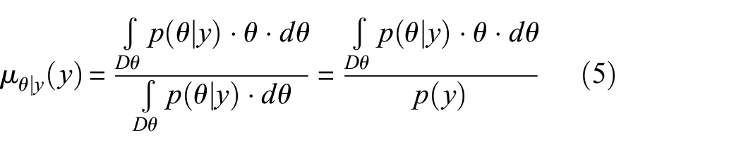
ShakeMaps have proven to be very effective tools for rapidly responding to earthquakes.² They are contour maps of several ground-motion parameters (also called intensity measures), such as peak ground acceleration and pseudo-spectral acceleration at different system periods estimated using empirical ground-motion prediction equations (GMPEs) based on information on the earthquake source (magnitude and location) and instrumental data from available seismic stations. Some examples of similar approaches include works by Gehl et al.,³ Michelini et al.⁴ and Bragato.⁵ ShakeMap information can also be combined with vulnerability curves (e.g. those provided by HAZUS⁶) for structural damage estimation in an area (see, for instance, the studies by Wald et al.² and Lagomarsino et al.⁷).

Structural health monitoring (SHM) systems have also been proven to provide useful information for rapid seismic damage assessment^8,9. Most existing SHM methodologies rely on the use of vibration measurements through accelerometers to detect potential structural damage.¹⁰ Encouraged by the recent technological developments in the field, global positioning system (GPS) receivers have also been increasingly used for damage detection.^11–14 Yet, associating damage with dynamic features is heavily restrained by the instrumentation layout/specifications, environmental effects and even the algorithms or methods used.^15–18 In addition to the specific sensing techniques focussed on a particular physical parameter, there are recent applications that make use of the multisensory environment and heterogeneous data for SHM.¹⁹ This can take the form of converting sensor information from one domain to another for corrected or enhanced^20–22 dynamic characterization, seeking changes in vibration behaviour as indicators of damage.

Seismic damage assessments should be carried out with probabilistic approaches, given the many uncertainties inherent to the problem. For example, even if the earthquake location and magnitude are known with good accuracy, significant uncertainty stems from the use of GMPEs.^23–27 Moreover, SHM sensor measurements are affected by noise, errors and have limited accuracy. Acknowledging the important role of uncertainties, in recent years an increasing number of studies have combined SHM and performance-based earthquake engineering (PBEE) concepts for rapid quantification of earthquake-induced building losses.^8,28–30

Bayesian modelling is a natural choice for carrying out rapid earthquake damage assessments, as it permits the propagation of uncertainties through models and allows updating the a priori estimates when new information becomes available. In particular, Bayesian networks (BNs) are ideal tools for describing the probabilistic relationships between the various parameters involved in the damage assessment and for integrating the available knowledge of the earthquake scenario and the structural response. In this context, Bayraktarli et al.,³¹ Bensi,³² Broglio et al.³³ and Gehl³⁴ proposed BN frameworks for risk assessment of urban infrastructure systems. Wu³⁵ developed a Bayesian framework for estimating the seismic damage in a structural system both before and after an earthquake, combining earthquake early warning and SHM data. Bayesian modelling can also be useful for quantifying the added value of the information provided by sensors and monitoring systems.^36–40 Approaches commonly employed for quantifying the reduction of uncertainty due to the available information are based on the concept of pre-posterior variance^36,40–42 or relative entropy reduction.⁴³

In this article, a probabilistic framework based on BNs is developed to quantify the benefit of various sensors for seismic damage assessment of critical structures under earthquake loading. The proposed framework relies on heterogeneous sources of information, such as those provided by seismometers typically used for deriving ShakeMaps, structure-mounted accelerometers and GPS receivers. The framework is applied to evaluate the seismic damage of a two-span bridge model located in a zone of high seismicity. To the authors’ knowledge, this is the first time that heterogeneous sensing techniques are used in a BN framework to update the estimates of the seismic losses of a system, and that the effectiveness of these sensing techniques is compared by using the pre-posterior variance and relative entropy reduction metrics.

The section ‘Seismic damage assessment’ illustrates in detail the various stages of the seismic damage assessment, the parameters involved and the technologies that are available to measure them. The section ‘Bayesian framework’ illustrates the BN developed to describe the relationship between the various parameters involved in the seismic damage assessment, and to update these parameters based on additional available information from different sources. It also presents the alternative approaches for quantifying the uncertainty reduction stemming from the sensor data. The section ‘Case study’ illustrates the implementation of the method on the two-span bridge considered as a case study. This is followed by a discussion of the results and the conclusion.

Seismic damage assessment

The Bayesian framework for seismic damage assessment combines four types of analyses, namely hazard analysis, structural analysis, response analysis and loss analysis, which is consistent with PBEE frameworks.^44,45 Since the focus of this study is the rapid damage assessment in the aftermath of an earthquake, the first stage is replaced by the assessment of the level of shaking at the site, given that the main characteristics of the earthquake are known. The subsequent subsections describe in more detail the four analysis stages, together with the involved parameters and the technologies for measuring them.

Seismic shaking analysis

This analysis provides an estimate of the probabilistic distribution of a given ground-motion parameter or intensity measure (IM) at the site of interest given the following variables that are assumed to be known: the moment magnitude of the earthquake (M_w); the epicentre of the earthquake, if a point-source event is assumed, or the rupture location and its extent for finite-fault scenarios; and other parameters characterizing the fault such as the faulting mechanism, the fault geometry and the depth to the top of the rupture. The analysis is carried out following the Bayesian procedure developed by Gehl et al.³ for generating ShakeMaps. A GMPE is used to estimate the ground motion at the site, given the earthquake’s characteristics. The GMPE is generally characterized by the following form²³

\log (I M_{i}) = f (M_{w}, R_{i}, s) + η + ζ_{i}

(1)

where $f (M_{w}, R_{i}, s)$ is a function describing the lognormal mean of $I M_{i}$ , that is, the IM at the location ‘i’, based on the earthquake magnitude M_w, a measure of the source-to-site distance R_i and other parameters collected in the vector s; η is the inter-event (or between-event) error term from the GMPE; and $ζ_{i}$ is the intra-event (or within-event) error term from the GMPE.

The interevent error term describes the systematic variability in the ground motions throughout the region produced by different earthquakes of the same magnitude and rupture mechanism. The intra-event error describes the variability in ground-motion intensity at various sites of same soil classification and distance from the source during a single earthquake.²⁴ Thus, following the studies by Park et al.²⁵ and Crowley et al.,²⁶ the same interevent variability is applied to all sites of interest within a given earthquake scenario, whereas the intra-event variability is represented by a spatially correlated Gaussian random field. This can be built based on the intra-event error terms $ζ_{i}$ and the correlation coefficient ρ_ij between the ground-motion parameters at two sites i and j, for i,j = 1,2,…N_sites, where N_sites is the number of sites of interest. The corresponding covariance matrix of the ground-motion IM field has the following form

Σ_{IM} = [\begin{matrix} σ_{η}^{2} + σ_{ξ i}^{2} & \dots & σ_{η}^{2} + ρ_{ij} σ_{ξ i} σ_{ξ j} \\ ⋮ & ⋱ & ⋮ \\ \dots & \dots & σ_{η}^{2} + σ_{ξ j}^{2} \end{matrix}]

(2)

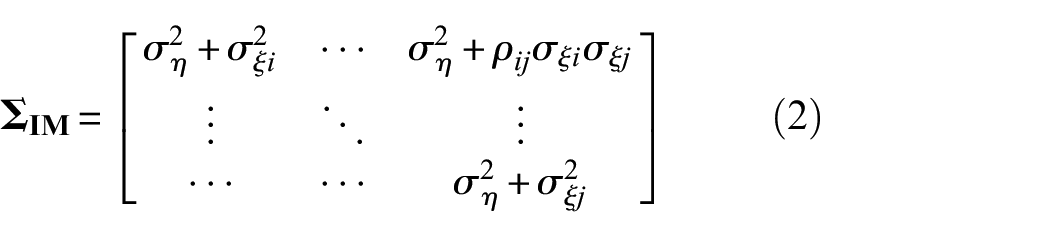
where σ_η and σ_ξ represent the standard deviations of the inter- and intra-event error terms, respectively, provided by the GMPE. Further details about this representation of the ground-motion field can be found in the study by Gehl et al.³ and in Schiappapietra et al.⁴⁶

The field observations of the ground-motion parameters at seismic stations can be used as evidence to update the prior estimates of the IM at the site of interest. The spatial correlation structure between the IMs at the monitored points and at the site plays a major role in the propagation of the observations.⁴⁷

Structural analysis

Structural analysis is performed to estimate the probabilistic distribution of one or more engineering demand parameters (EDPs), describing the response of structural and non-structural components, based on the seismic shaking intensity. A joint probabilistic seismic demand model should be considered to describe the relationship between the EDPs and the IM, by also accounting for the correlation between the various EDPs. This is very important because the correlation structure is a basis for updating the probabilistic distribution of one EDP (e.g. floor acceleration in a building) given the observation of another (e.g. storey drift).

Alternative approaches can be employed to develop the joint probabilistic seismic damage model (PSDM), such as multi-stripe analysis,⁴⁸ incremental dynamic analysis,⁴⁹ or cloud analysis.⁵⁰ In this study, cloud analysis is adopted. For this purpose, the structural model is analysed under a set of ground-motion records of different IM levels. The samples of the various response parameters (EDP_i, for i = 1,2,…,N_EDP) are then fitted by a regression model. In particular, a bilinear model is considered in this study,^51,52 since it allows a better description of the evolution of the structural response with the seismic intensity. The model for the generic ith EDP has the following form (see Figure 1)

\begin{matrix} \ln (ED P_{i} | IM) = [a_{1} + b_{1} \ln (IM) + \ln ε_{1}] H (IM - IM *) \\ + [a_{1} + b_{1} \ln (IM *) + b_{2} (\ln (IM) - \ln (IM *)) + \ln ε_{2}] \\ [H (IM * - IM)] \end{matrix}

(3)

in which a₁ is the intercept of the first segment, b_i for i = 1, 2 are the slopes of the two segments (see Figure 1), $IM *$ is the breakpoint IM, which is defined as the point of intersection of the two segments. The step function $H (g)$ controls which of the two segments must be considered (i.e. H = 0 for $IM \leq IM *$ and H = 1 for $IM > IM *$ ). The probability distribution of each EDP is also described by the values of the error functions $ε_{i}$ , which are characterized by a lognormal distribution with lognormal zero mean and lognormal standard deviations $β_{i}$ . Moreover, in order to define a joint probability density function (PDF) for the various EDPs, a covariance matrix must be assigned, which has the same form as that of equation (2). For this purpose, different correlation coefficients must be estimated for the two conditions corresponding to $IM \leq IM *$ and $IM > IM *$ , thus leading to two correlation matrices, $\sum_{EDP}^{I}$ and $\sum_{EDP}^{II}$ .

Figure 1.

Illustration of the bilinear regression model.

A brief description of the EDPs considered in this study and relevant measurement techniques is given below. Table 1 summarizes the EDPs of interest and possible sensors to collect observations directly and indirectly.

Table 1.

Engineering demand parameters and measurement possibilities.

EDP	Component performance	Direct measurement	Indirect measurement
Peak transient displacement (TD)	Global structural components, non-structural components	GPS receivers, laser vibrometer, transducers, camera	Accelerometers
Residual displacement (RD)	Global structural components	GPS receivers, laser vibrometer, transducers, camera	Accelerometers
Peak absolute acceleration (PA)	Non-structural building components, bridge deck	Accelerometers	GPS receivers

EDP: engineering demand parameter; GPS: global positioning system.

Peak transient displacements

The maximum absolute values of the transient displacements (or of geometrically derived quantities, such as drifts) during the time history of motion of a structure are important indicators of structural performance. Many vulnerability curves for structures are based on these EDPs. Peak transient displacements (TDs) can be derived from the time histories of structures’ relative displacements with respect to the base, and a wide range of sensors (both contact and non-contact) can be used to measure them.

Lemnitzer et al.⁵³ employed transducers such as linear variable differential transformers (LVDTs) to measure the shear deformations of a wall across two floors of a building, whereas Li et al.⁵⁴ proposed the use of smartphone cameras. Trapani⁵⁵ developed SAFEQUAKE, a hinged bar instrumented with two bi-axial accelerometers measuring accelerations, one at each end of the beam and remaining parallel to the building floors, and one bi-axial inclinometer or accelerometer measuring the tilt of the beam. There are also some applications of GPS systems for real-time monitoring of displacement measurements. However, GPS technology is limited by low sampling rates and because it only measures the displacements at the building roof or bridge deck level.⁵⁶

Residual displacements

The residual drift or permanent deformations of structural components after the earthquake may be used to infer the degree of damage sustained by the structure. Many studies have investigated the correlation between maximum drifts and residual displacements (RDs; see study by Dai et al.⁵⁷ for a recent review on the topic). However, most of these studies have aimed at developing empirical formulae to relate the RDs and TDs and to provide a deterministic relation between the two EDPs, without any information regarding the dispersion⁵⁸ nor any consideration of its dependence on the seismic intensity. Probabilistic studies relating TDs and RDs or drifts are scarce. Goda⁵⁹ developed a joint PDF for the probability distribution of TD and RD seismic demands using a copula. Ruiz-García and Miranda⁶⁰ evaluated and compared demand hazard curves for residual drifts and maximum transient drifts in multi-storey building frames. Uma et al.⁶¹ developed a probabilistic performance-based seismic assessment framework where the performance levels defined by pairs of maximum-residual deformations are derived using bivariate probability distributions. Yazgan and Dazio⁶² proposed a Bayesian approach for post-earthquake damage assessment using the information from known RDs to update the probability distribution of maximum transient drifts in building frames.

Peak absolute accelerations

Many non-structural components in buildings are damaged during earthquakes when subjected to large absolute acceleration demands rather than high drift demands. Suspended ceilings, parapets and light fixtures are typical building components sensitive to accelerations. Along with masonry infills, ceiling systems are the non-structural elements most prone to damage during an earthquake. Absolute accelerations are typically measured via accelerometers. Accelerations may also be derived by differentiating velocities and displacements but obtaining reliable estimates can be problematic unless smooth velocity or displacement signals with high sample rates are available.

Excessive bridge accelerations can cause serviceability problems, and in case of an earthquake, may distort operational flow (e.g. driver safety⁶³). Although mostly disregarded, vertical bridge accelerations can sometimes be excessive and may necessitate external devices for control.⁶⁴

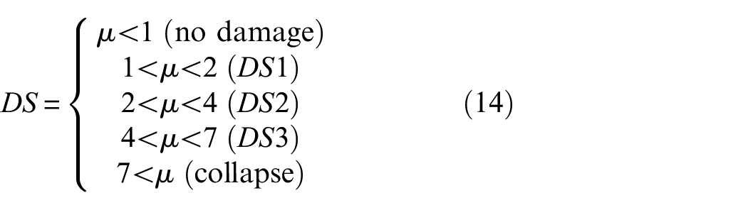
Damage analysis

In this stage, the EDPs are used to estimate the level of damage of the structure, typically described by one or more damage states (DSs). In buildings, damage of structural components can be described as a function of the peak inter-storey drift ratio, and that of non-structural components based on the peak absolute accelerations (PAs).^29,65 In bridges, the damage of the bearings, shear keys, columns and abutments is controlled by kinematic quantities, such as displacements and curvatures. Bridge piers are often the most vulnerable components of a bridge^66,67 and their damage can be expressed as a function of the peak drift ratio⁶⁸ or it can be related to the maximum displacement ductility experienced.^69,70

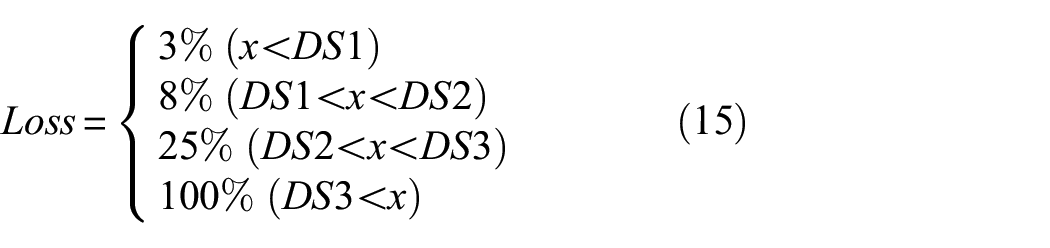
Loss analysis

In this final stage, various decision variables (DVs) can be calculated, such as repair cost, casualties and loss-of-use duration (money, deaths and downtime), based on the damage sustained by the structural components. Padgett et al.⁷¹ after Basöz and Mander⁷² associated loss levels with damage measures experienced by bridges. Lu et al.⁷³ pursued a similar loss assessment scheme for buildings with multi-class damage descriptions. Similar to these studies, in this article, structural losses related to damage are formulated in terms of loss ratios (LRs), repair and replacement costs normalized by the bridge cost.

Bayesian framework

This section presents the Bayesian framework developed for near real-time loss assessment and describes the methods used for quantifying the effectiveness of sensors for uncertainty reduction.

Bayesian network

This subsection illustrates the BN developed to describe the probabilistic relationship between the parameters specified in the previous section, to perform predictive analysis and to update these parameters based on additional information from different observations (see Figure 2). The magnitude M_w and epicentre of the earthquake are assumed to be known, and three different types of information are assumed to be available to update the probabilistic relationship of the variables in the network: on-site seismometers located close to the site of the structure, providing information on IM levels; GPS data, updating the knowledge of the RD; and accelerometer data, updating the knowledge of the PA in the bridge deck.

Figure 2.

Bayesian network illustrating the relationship between the parameters involved in the damage and loss assessment (observed quantities indicated with thick lines).

The nodes of the BN represent random variables characterized by a PDF. In particular, nodes are related to their parent and child variables through edges stating conditional dependencies between variables (i.e. use of conditional probability distributions). The nodes that have no parents are termed as root nodes and they are associated with marginal probability distributions. Node junction patterns can take different forms such as collider (M_w and R to IM), fork (IM to EDPs) and chain (TD to damage, damage to loss) with varying dependency features. Two forms of probabilistic inference can be carried out in BNs: predictive analysis that is based on evidence (i.e. information that the node is in a particular state) on root nodes and diagnostic analysis, also called Bayesian learning, where observations enter into the BN through the child nodes. When evidence enters the BN, it is spread inside the network thereby updating the probability distribution of the variables through one of the two forms of inference mentioned above.

The seismic shaking is modelled by the deterministic root nodes that describe the magnitude of the earthquake event, M_w, and the vector $R_{e}$ that collects the distances between the source and the site, and the source and the seismic stations. For demonstration purposes, two seismic stations (represented by IM₂ and IM₃) are assumed here to be in the vicinity of the bridge site (represented by IM₁).

Following the study by Gehl et al.,³ the interevent variability is modelled by the root node W, which is parent to the three IMs of interest (i.e. the one at the site and the ones at the seismic stations) and follows a normal standard distribution. The intra-event variability is modelled via three root nodes, U_j, for j = 1,2,3, which also follow a normal standard distribution. The joint conditional distribution of the IMs, given W and U_i, can be expressed by the following relation

\begin{matrix} \ln (I M_{i} | W, U_{j}) = \ln \bar{I M_{i}} (M_{w}, R_{i}) + σ_{ξ} \sum_{j = 1}^{3} t_{ij} U_{j} + σ_{η} W \\ i = 1, 2, 3 \end{matrix}

(4)

where $\bar{I M_{i}}$ is the median value of the IM and $\ln \bar{I M_{i}} (M_{w}, R_{i})$ is the lognormal mean, which is a function of $M_{w}$ and $R_{i}$ (see also equation (1)); $σ_{ξ}$ and $σ_{η}$ are the lognormal standard deviations describing, respectively, the intra-event and interevent variability; $t_{ij}$ is a term of the lower triangular matrix obtained through a Cholesky factorization of $C_{IM}$ , which is the spatial correlation matrix expressing the correlation between the IMs at the various sites.

A similar approach is used for the PSDM describing the conditional distribution of the EDPs given the IM at the site, IM₁. However, in this case, a bilinear model is employed, and thus two different error variables and correlation matrixes have to be considered, one for $I M_{1} < IM *$ and the other for $I M_{1} > IM *$ . Two other root nodes, denoted as e_GPS and e_ACC, are used to describe the measurement errors of the observations obtained with GPS and accelerometers. These error variables are assumed to be zero-mean normally distributed variables. Finally, a damage model is employed to describe the conditional relationship between the various DSs of the system and the EDPs, and a loss model to relate the losses to damage.

The BN detailed in Figure 2 is used to perform predictive analysis, starting from the prior distribution of the root nodes, and diagnostic analysis, entering an observation at the nodes IM₂, IM₃, RD_obs and PA_obs. For this purpose, the OpenBUGS software⁷⁴ is employed, which is interfaced with the R statistical tool. OpenBUGS is able to treat both deterministic (e.g. M_w and $R_{e}$ ) and probabilistic (e.g. IM_i, ln(TD)) variables, which are sampled through a Markov-chain Monte-Carlo (MCMC) sampling scheme. Each chain is built with a Gibbs sampling scheme, where variables are successively sampled from the posterior distribution of previous variables: the posterior distribution of a variable is obtained from the product of the prior distribution and the likelihood function (probability of a given observation occurring given the prior distribution). The samples are then aggregated in order to estimate empirical statistics of the variables of interest, which represent the posterior distributions. Although Bayesian inference based on sampling provides only approximate solutions (i.e. the posterior distribution is built from the samples), it has the benefit of being much more flexible than exact inference algorithms such as junction-tree inference (e.g. it allows modelling continuous variables using various probability distributions). Due to the approximate nature of the posterior distributions sampled by the MCMC scheme, there is no absolute guarantee that exact distribution parameters may be obtained. However, various steps may be taken in order to ensure a reasonable accuracy of the results:

Generation of multiple MCMC chains starting with different combinations of initial conditions, in order to ensure that all chains end up converging towards the same values.

Generation of a high number of samples for each chain (e.g. several tens of thousands).

Definition of a ‘burn-in phase’, where the first part of each chain is taken out from the estimation of the posterior distribution, in order to remove samples that have not yet converged.

Thinning of the samples (i.e. only one sample in every five is considered in each chain), in order to reduce autocorrelation effects that are inherent to MCMC sampling.

Specific statistical tools in OpenBUGS are dedicated to the estimation of auto-correlation and of the minimum number of samples. In any case, preliminary tests are necessary to calibrate the sampling parameters carefully. The chosen sampling results from a trade-off between the required accuracy level and the computational cost.

Quantification of sensors’ effectiveness for uncertainty reduction

Pre-posterior variance

The effectiveness of the monitoring strategy can be described based on the concept of pre-posterior variance,⁴¹ which represents the expected value of the variance of the random variable of interest (e.g. EDP) after monitoring is performed, that is, after Bayesian updating is carried out based on the available information. The pre-posterior variance accounts for all the possible combinations of outcomes of the monitoring system and thus it is independent of any specific observation. Compared with the prior variance, the pre-posterior variance gives an idea of how useful the monitoring process is in gaining information on the unknown parameter. A pre-posterior variance much smaller than the prior indicates that the proposed monitoring method improves our knowledge of the parameter. On the contrary, similar values of the pre-posterior and prior variances indicate that monitoring is not expected to bring any significant knowledge improvement.

Let $p (θ)$ denote the prior distribution of a generic random variable $θ$ , such as a node of the BN which is not deterministic, and $p (θ | y)$ the posterior distribution, following an observation y. The expected value and variance of the posterior distribution of $θ$ can be expressed as

μ_{θ | y} (y) = \frac{\int_{D θ} p (θ | y) \cdot θ \cdot d θ}{\int_{D θ} p (θ | y) \cdot d θ} = \frac{\int_{D θ} p (θ | y) \cdot θ \cdot d θ}{p (y)}

(5)

σ_{θ | y}^{2} (y) = \frac{\int_{D θ} p (θ | y) \cdot {(θ - μ_{θ | y} (y))}^{2} \cdot d θ}{p (y)}

(6)

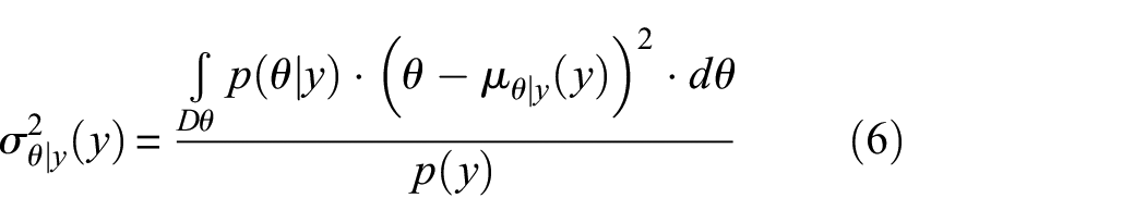
Since the observation is unknown a priori, these quantities can be seen as function of the observation y. The pre-posterior variance can be obtained by taking the expectation with respect to y

\begin{matrix} σ_{θ, PP}^{2} = E [σ_{θ | y}^{2} (y)] = \int_{Dy} σ_{θ | y}^{2} (y) \cdot p (y) \cdot dy \\ = \int_{D (θ, y)} p (θ | y) \cdot {(θ - μ_{θ | y} (y))}^{2} \cdot d θ \cdot dy \end{matrix}

(7)

In practice, $σ_{θ, PP}^{2}$ can be estimated with a Monte-Carlo approach. For this purpose, a set of possible monitoring scenarios are generated by performing predictive analysis and generating multiple samples of the possible observations. Each observation is then used as input in a diagnostic analysis to produce a sample of the posterior distribution of the variable of interest. The pre-posterior variance is then obtained by averaging the values of $σ_{θ | y}^{2} (y)$ obtained for the different observations.

The expected effectiveness of the monitoring system is measured by the square root of the ratio between the prior and the pre-posterior variances

η = \sqrt{\frac{σ_{θ}^{2}}{σ_{θ, PP}^{2}}} = \frac{σ_{θ}}{σ_{θ, PP}}

(8)

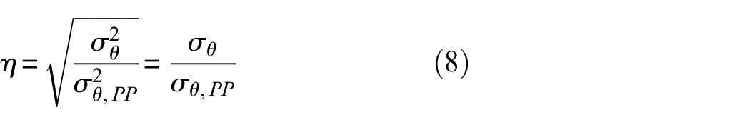
This synthetic parameter can be used to compare the reduction of uncertainty in the estimation of $θ$ obtained via alternative monitoring techniques, and can also be used to evaluate the benefits of fusing the data from different sensors. It can be demonstrated that this parameter is always higher than 1, even though for some observations y the ratio between $σ_{θ}^{2}$ and $σ_{θ | y}^{2} (y)$ can be less than 1.

Reduction of relative entropy

As an alternative to the pre-posterior analysis approach, a relative entropy measure can be used to quantify the information gain from the available observations. Relative entropy, also called Kullback–Leibler divergence, expresses the difference between two probability distributions when identifying the value of new information or more specifically, observations.^75,76,43 According to Shannon, the information entropy for a random variable θ with posterior distribution $p (θ | y)$ is defined as the following

H [p (θ | y)] = - \int_{D_{θ}} \ln [p (θ | y)] p (θ | y) d θ

(9)

The cross entropy between two posterior and prior probability distributions, which measures the expected information that is required to get from one distribution to another, is

H [p (θ | y), p (θ)] = - \int_{D_{θ}} \ln [p (θ)] p (θ | y) d θ

(10)

The relative entropy $D_{KL} [p (θ | y), p (θ)]$ measures the so-called information geometry in moving from the prior to the posterior and can be expressed as

\begin{matrix} D_{KL} [p (θ | y), p (θ)] = H [p (θ | y), p (θ)] - H [p (θ | y)] \\ = \int_{D_{θ}} \frac{\ln [p (θ)]}{\ln [p (θ | y)]} p (θ | y) d θ \end{matrix}

(11)

According to the formulation, the relative entropy of the observation and reference distribution is lower bounded by 0. In other words, the greater the difference between the two probability distributions, the greater the relative entropy gained from the arrival of observational data. As for the case of the pre-posterior variance, the relative entropy is estimated via a Monte-Carlo approach by averaging all the possible monitoring outcomes. Thus, the obtained effectiveness measure is independent of the specific observation y.

Case study

In this section, the application of the framework presented above to a bridge structure is described.

Case study description

Structural system model for damage and loss assessment

For demonstration purposes, the structural system considered in this study consists of a two-span bridge with a continuous multi-span steel–concrete composite deck, arbitrarily located in the area of Patras, Greece (longitude 21.906, latitude 38.278, in decimal degrees). The bridge is representative of a class of regular medium-span bridges commonly used in transportation networks^77–78 (see Figure 3). The bridge superstructure, designed according to the specifications given in Eurocode 4,⁷⁹ consists of a reinforced concrete slab of width B = 12 m, which hosts two traffic lanes, and of two steel girders positioned symmetrically with respect to the deck centreline at a distance of 6 m. Class C35/45 concrete is used for the superstructure slab. The reinforcement bars are made of grade B450C steel, and the deck girders are made of grade S355 steel. The distributed gravity load due to the self-weight of the deck and of non-structural elements is 138 kN/m, for a weight per unit length m_d = 14.07 ton/m. The reinforced concrete piers have a circular cross-section of diameter D = 1.8 m. They are made of class C30/37 concrete, with a longitudinal reinforcement steel ratio of 1% and a transverse reinforcement volumetric ratio ρ_w = 0.5%. Further details about the bridge can be found in the study by Tubaldi et al.⁷⁸

Figure 3.

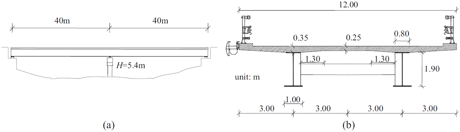
(a) Two-span bridge profile and (b) transverse deck section.

A three-dimensional finite element (FE) model of the bridge is developed in OpenSees⁸⁰ following the same approach described in the study by Tubaldi et al.,⁶⁶ that is, using linear elastic beam elements for describing the deck, and the beam element with inelastic hinges developed by Scott and Fenves⁸¹ to describe the pier. Further details of the FE model and of the pier properties are given in the study by Tubaldi et al.⁶⁶ The elastic damping properties of the system are described by a Rayleigh damping model, assigning a 2% damping ratio at the first two vibration modes. The FE model described in this study is assumed to be deterministic and characterized by no epistemic uncertainties. Future extensions of the methodology will consider how introducing some uncertainty in the model (e.g. considering the approach outlined by Tubaldi et al.⁶⁷) would affect the results.

Figure 4 shows the hysteretic response of the pier to a bi-directional ground-motion record, in terms of moment–curvature of the base section, and base shear–top displacement, along the two principal directions of the bridge. It can be observed that the model is characterized by some degradation of stiffness and pinching, that results from the constitutive model adopted to describe the concrete fibres in the plastic hinge region (Concrete 02 in OpenSees⁸⁰). A more sophisticated description of the hysteretic behaviour of the pier is out of the scope of this study.

Figure 4.

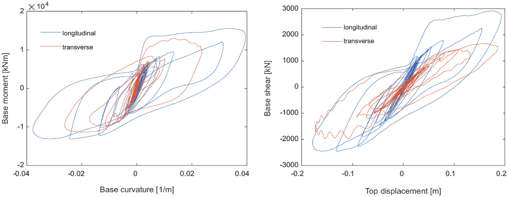
(a) Base moment–curvature response and (b) base shear–top displacement response.

A set of 221 ground-motion records is used to derive the PSDM: 120 of these were selected by Baker et al.⁸² for the performance assessment of a variety of structural systems located in active seismic regions. These records are representative of a wide range of variation in terms of source-to-site distance (R) (from 8.71 to 126.9 km), soil characteristics (the average shear wave velocity V_S in the top 30 m of soil spans from 203 to 2016 m/s) and moment magnitude (M_w) (from 5.3 to 7.9), so as to obtain more robust and general results. It is noted that the V_S values of many of these records are higher than those assumed for deriving the seismic shaking scenarios considered here. This approach, potentially resulting in some bias in the estimation of the PSDM, is consistent with current practice. An alternative approach would have been to select records based on the actual soil conditions at the bridge site and on the actual seismotectonic context around the site. It would have been difficult to find sufficient records to build an accurate PSDM if this approach had been followed. The remaining ground motions are taken from the recordings of different stations during the 1994 Northridge earthquake and they were added to achieve a more confident estimate of the response for high IM values. The large number of records in the set allows estimation with good confidence of the statistics of the response parameters, even of those which are characterized by a significant dispersion such as the RD.⁴⁸ The median horizontal (geometrical mean) spectral displacement response S_d(T) at the fundamental period of the bridge (T = 0.45 s) for a damping ratio of 2% is selected as the IM. It is noteworthy that the GMPE by Akkar and Bommer,⁸³ which is used in this study, is formulated in terms of the pseudo-spectral acceleration S_a(T), which is related to S_d(T) through the expression $S_{d} (T) = S_{a} (T) / ω^{2}$ , where $ω$ = 2π/T. An amplification factor $= 1.195$ is used to account for a 2% damping factor instead of 5%, based on the expression for the damping reduction factor taken from Eurocode 8.⁸²

The PSDM described in the section ‘Structural analysis’ is fitted to the 221 samples of the various response parameters of interest for the performance assessment, namely the RD (EDP₁ = RD), the TD (EDP₂ = TD) and the PA (EDP₃ = PA). Figure 5 shows the sample values of the EDPs versus IM in the log–log plane and in the untransformed plane. In the same figures, the lognormal mean and median of the fitted PSDM are also plotted. The same value of IM* is used for various EDPs. It is obtained by considering the samples of the RDs, since the change of slope is more evident from these. In fact, for $IM \leq IM *$ the response of the system is in the linear range, and the RDs are zero, whereas for $IM > IM *$ the RDs assume values different from zero and increase for increasing IM levels. It is noteworthy that the value of $IM *$ = 0.0286 m corresponds on average to a drift ratio of 0.68% (defined as the ratio between the TD and the pier height), which signals the onset of nonlinearity of the system due to concrete cracking and rebar yielding. The peak top displacements and the absolute accelerations increase almost linearly with the seismic intensity and their trend of variation does not change significantly when IM exceeds $IM *$ .

Figure 5.

Sample values and model results in terms of RD, TD and PA versus IM in the log–log plane (left column) and in the untransformed plane (right column).

The covariance matrices $\sum_{EDP}^{I}$ and $\sum_{EDP}^{II}$ , collecting the information on the variance of the error variables (in the lognormal space) and on their correlation, for the two branches of the PSDM (corresponding, respectively, to $I M_{1} \leq IM *$ and $I M_{1} > IM *$ ) are

\begin{matrix} \sum_{EDP}^{I} = [\begin{matrix} 3.700 & 0.271 & 0.039 \\ 0.270 & 0.222 & 0.114 \\ 0.039 & 0.114 & 0.156 \end{matrix}] \\ \sum_{EDP}^{II} = [\begin{matrix} 2.875 & 0.612 & 0.203 \\ 0.612 & 0.293 & 0.126 \\ 0.203 & 0.126 & 0.098 \end{matrix}] \end{matrix}

(12)

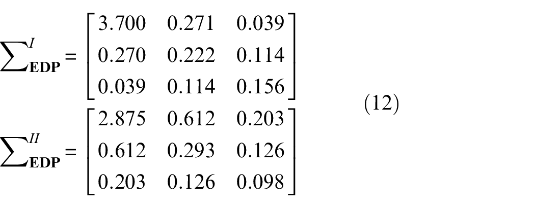
and the corresponding correlation matrices are

\begin{matrix} C_{EDP}^{I} = [\begin{matrix} 1 & 0.299 & 0.0516 \\ 0.299 & 1 & 0.611 \\ 0.051 & 0.611 & 1 \end{matrix}] \\ C_{EDP}^{II} = [\begin{matrix} 1 & 0.667 & 0.382 \\ 0.667 & 1 & 0.744 \\ 0.382 & 0.744 & 1 \end{matrix}] \end{matrix}

(13)

It can be observed that the RDs are characterized by significant dispersion, which is much higher than that of the other EDPs. Moreover, the correlation between the error variable in the PSDM of RD and the error variable in the PSDMs for the other EDPs is quite low for $I M_{1} \leq IM *$ , but it increases for $I M_{1} > IM *$ . This is expected, since for $I M_{1} \leq IM *$ the residual drifts are very low. The highest correlations are observed for high seismic intensities between the errors for the PSDMs of RD and TD (correlation coefficient of 0.667 for the second branch of the PSDM) and for the PSDMs of TD and PA (correlation coefficient of 0.774). The correlation between RD and PA is quite low, though not negligible for high seismic intensities (correlation coefficient of 0.382). This suggests that the information on accelerations may be used to reduce uncertainty in the estimation of the bridge’s TDs and RDs. It is noteworthy that the proposed approach is different from resorting to double integration of the measured acceleration signal for estimating the displacements, which is characterized by several limitations.⁸⁵

The damage of the bridge is assumed to be controlled by the pier. Similar to the study by Choi et al.,⁶⁹ the pier damage is expressed as a function of the ductility demand as follows

DS = {\begin{matrix} μ < 1 (no damage) \\ 1 < μ < 2 (DS 1) \\ 2 < μ < 4 (DS 2) \\ 4 < μ < 7 (DS 3) \\ 7 < μ (collapse) \end{matrix}

(14)

where $μ$ and $DS$ denote, respectively, the ductility demand and the damage state of the bridge. The relationship between the pier top displacement TD and the ductility demand $μ$ is evaluated by performing pushover analysis of the bridge in the longitudinal direction.

The losses are obtained using the equation below^71,72

Loss = {\begin{matrix} 3 % (x < DS 1) \\ 8 % (DS 1 < x < DS 2) \\ 25 % (DS 2 < x < DS 3) \\ 100 % (DS 3 < x) \end{matrix}

(15)

Seismic scenarios and field observations

It is assumed that the bridge is equipped with one accelerometer and one GPS antenna, both mounted at the level of the superstructure above the pier. The measurement error of the GPS antenna is characterized by a normal distribution with zero mean and a standard deviation of 1 mm, whereas that of the accelerometer is characterized by a normal distribution with zero mean and a standard deviation of 0.002 m/s². These values are based on the noise root mean square (RMS) levels of exemplary low-cost sensor specifications extracted from representative datasheets (refer to⁸⁶ for the noise of a global navigation satellite system (GNSS)-based displacement measurement device and STMicroelectronics⁸⁷ for a low-cost micro electro-mechanical systems (MEMS) accelerometer). The hypothetical bridge is located close to two existing seismic stations (see Figure 6). The first one (PATRA-C) is at the latitude 38.269 and longitude 21.760, whereas the second one (RIO) is at the latitude 38.296 and longitude 21.791. These coordinates correspond to a distance between the site and PATRA-C of 12.8 km, and between the site and RIO of 10.2 km. The distance between the two stations is 4 km.

Figure 6.

Map with indications of bridge site, seismic point sources for scenarios 1 and 2, and seismic stations.

The seismic hazard at the site is quantified by considering the seismic source zonation of the European Seismic Hazard Model 2013.⁸⁸ The earthquake scenarios used in the subsequent sections are two possible realizations obtained by sampling from this model. The prediction of the ground motions at the site from the considered earthquake point sources is made using GMPE by Akkar and Bommer,⁸³ assuming soft soil conditions (V_s < 360 m/s) and a strike-slip fault mechanism. The spatial correlation model proposed by Jayaram and Baker⁴⁷ is used to build the correlation matrix C_IM expressing the correlation between the IMs at different sites. The terms of C_IM are the correlation coefficients ρ_ij between the ground-motion parameters at two sites i and j, expressed as

ρ_{ij} = \exp (- \frac{3 r_{ij}}{b})

(16)

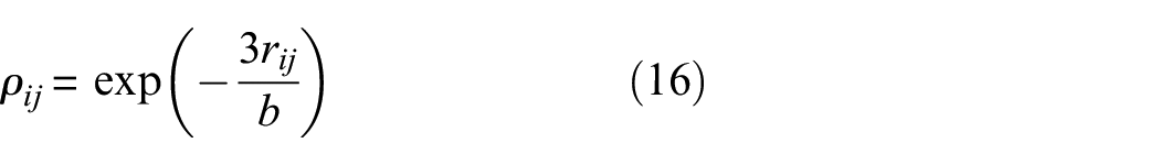
in which r_ij is the distance between the sites and b is the correlation distance.

It is noteworthy that the correlation distance varies significantly from site to site and from earthquake to earthquake, and it also changes with the structural period.⁴⁶ Equations for capturing the dependence of b on these parameters are provided by Jayaram and Baker,⁴⁷ from which the value of b for this study (15.9 km) is taken.

As a result, the covariance matrix $Σ_{IM}$ related to the IMs (IM₁, IM₂, IM₃ corresponding, respectively, to the bridge site, and the PATRA-C and RIO stations) in lognormal space, as well as the spatial correlation matrix $C_{IM}$ between the sites, are estimated as follows

\begin{matrix} Σ_{IM} = [\begin{matrix} 0.105 & 0.021 & 0.026 \\ 0.021 & 0.105 & 0.056 \\ 0.026 & 0.056 & 0.105 \end{matrix}] \\ C_{IM} = [\begin{matrix} 1 & 0.089 & 0.146 \\ 0.089 & 1 & 0.470 \\ 0.146 & 0.470 & 1 \end{matrix}] \end{matrix}

(17)

It is worth noting that the correlation values between the sites are very low, which is due to the quickly decreasing spatial correlation model. However, the arbitrary case study that is defined here is consistent with the usual seismic network density in Europe (e.g. exposed sites are often a dozen kilometres or more away from the nearest seismic station). Since the information gain provided by the seismic stations in terms of uncertainty reduction at the bridge site is expected to be low due to the low correlation between IM₁ and IM₂ and IM₃, the case of a ground accelerometer placed at the base of the bridge is also considered to quantify the maximum uncertainty reduction achievable by a perfect knowledge of the IM₁.

Rapid damage assessment for a single scenario

This subsection describes the results of the Bayesian updating for scenario 1, which corresponds to the seismic point source 1, with Magnitude M_w 5, located 28.0 km from the site and 40.6 and 38.2 km from the stations PATRA-C and RIO, respectively (Figure 6).

Predictive analysis is first run based on the information at the root nodes (including the deterministic ones, M_w and R_e, that describe the earthquake scenario). Subsequently, multiple independent diagnostic analyses are performed by entering a piece of evidence one at a time at the nodes IM₂, IM₃, RD_obs and PA_obs and also by entering all the information at these nodes at the same time. These analyses are performed with OpenBugs⁷⁴ using three MCMC chains generated with different combinations of initial conditions. This is to ensure that the three different starting points converge towards similar posterior distributions. Each chain contains 10,000 samples, which are obtained by starting from 60,000 iterations, discarding the first 10,000 (burn-in) and thinning to reduce autocorrelation. Ultimately, a total of 30,000 samples is used to estimate the posterior distributions. It is noteworthy that the time required to perform a single Bayesian Inference analysis is quite low (of the order of a few seconds on a standard personal computer.

Figure 7 shows the empirical cumulative distribution function (CDF) for the prior distribution of the various parameters of interest, and the posterior distributions given the observations of the GPS, accelerometers (Acc) and seismic stations (Map). The results obtained by combining the observations are also shown for comparison (Com). Table 2 reports median values and standard deviations of the prior and posterior distributions, together with the observations from the various sensors.

Figure 7.

Empirical cumulative distribution function (CDF) of the parameters of interest before and after updating with observations from scenario 1.

Table 2.

Median and lognormal standard deviation of prior and posterior distribution of parameters of interest for a realization from scenario 1.

Observation source	Observation	RD		TD		PA		IM		LR
Observation source	Observation	Median (m)	β	Median (m)	β	Median (m/s²)	β	Median (m)	β	Median (–)	β
None (prior)	–	1.22 × 10⁻⁵	2.873	0.0031	0.845	0.389	0.704	0.0019	0.744	0	0
Seismic stations	0.0011 m, 0.0000596 m	1.20 × 10⁻⁵	2.877	0.00270	0.828	0.351	0.696	0.0017	0.724	0	0
GPS	2.8 × 10⁻⁴ m	1.02 × 10⁻⁵	2.599	0.00260	0.834	0.343	0.691	0.0016	0.726	0	0
Accelerometer	0.672 m/s²	1.60 × 10⁻⁵	2.897	0.00449	0.406	0.695	0.029	0.0028	0.447	0	0
Combined	–	1.45 × 10⁻⁵	2.491	0.005	0.446	0.694	0.029	0.0028	0.486	0	0

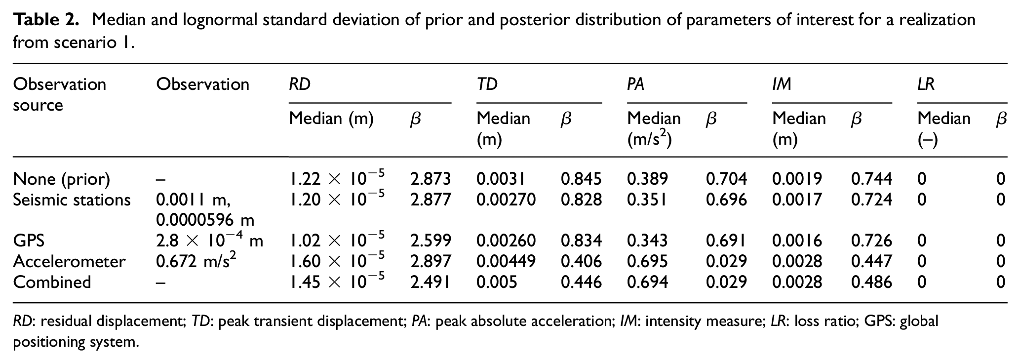
RD: residual displacement; TD: peak transient displacement; PA: peak absolute acceleration; IM: intensity measure; LR: loss ratio; GPS: global positioning system.

The prior distribution is characterized by low values of the various EDPs, as expected, given the low magnitude and high epicentral distance of the source. Thus, the expected losses are zero. The RDs are very small, though significantly dispersed, with a value of lognormal standard deviation β of the order of 2.8, whereas the other parameters are characterized by smaller dispersion, with values of β of the order of 0.7–0.8. The information from the sensors generally results in a reduction of the uncertainty, corresponding to a steeper empirical CDF for the posterior distributions of the parameters of interest compared to the prior, and to a reduced lognormal standard deviation. The use of an accelerometer clearly outperforms the other sensing strategies in terms of uncertainty reduction. In particular, using the accelerometer, the dispersion of the absolute acceleration of the deck reduces from 0.7 to about 0.03, but the dispersion of the RDs remains unvaried, due to the low correlation between accelerations and RDs for low seismic intensities, when the RDs are very low. The reduction of uncertainty of the RDs is not significant even if GPS data are used, due to the significant noise-to-signal ratio, thus resulting in a reduction in the dispersion of the residual only by 10%. The overall reduction of uncertainty is more significant if the combined observations from the various sensors are used. However, there is only a minimal improvement by considering additional information from other sensors if the accelerometers are already used, as demonstrated by the fact that the distributions of all the EDPs, with the exception of the RD for the Acc and Com cases, almost overlap.

A larger earthquake (scenario 2) is considered, which corresponds to a realization generated considering seismic point source 2, with magnitude M_w 6.5, located 20.7 km from the site and 14.6 and 12.7 km from the stations PATRA-C and RIO, respectively (Figure 6). The results corresponding to this realization are shown in Figure 8 and in Table 3.

Figure 8.

Empirical cumulative distribution function (CDF) of the parameters of interest before and after updating with observations from scenario 2.

Table 3.

Median and lognormal standard deviation of prior and posterior distribution of parameters of interest for a realization from scenario 2.

Observation source	Observation	RD		TD		PA		IM		LR
Observation source	Observation	Median (m)	β	Median (m)	β	Median (m/s²)	β	Median (m)	β	Median (–)	β
None (prior)	–	9.2 × 10⁻⁵	2.672	0.042	0.857	2.76	0.696	0.0272	0.744	0	0.04
Seismic stations	0.0627 m, 0.0904 m	6.67 × 10⁻⁴	3.0744	0.077	1.040	4.826	0.855	0.0486	0.947	0.08	0.5
GPS	5.4 × 10⁻⁴ m	0.00023	1.841	0.057	0.702	3.955	0.607	0.0429	0.719	0.03	0.125
Accelerometer	8.103 m/s²	0.0195	2.52	0.194	0.437	8.1	0.002	0.122	0.807	1	1.097
Combined	–	0.0008	0.919	0.101	0.172	8.1	0.002	0.065	0.282	0.25	1.339

RD: residual displacement; TD: peak transient displacement; PA: peak absolute acceleration; IM: intensity measure; LR: loss ratio; GPS: global positioning system.

In this case, the prior distribution is characterized by relatively high values of the TD, resulting in a median drift ratio of 0.78%, which corresponds to an inelastic behaviour of the pier. However, the median value of the RD is still very low, as a result of the hysteretic behaviour of the pier and the stiffness degradation and pinching (see Figure 4). The realization considered is characterized by a high value of the observation of the accelerometer compared to the prior median estimate, which results in an increased median value of PA and of the other response parameters compared to the prior one. It is noteworthy that the posterior CDFs of all the monitored random variables (with the exception of the absolute accelerations) updated considering the observation of the accelerometer are characteristic of a bimodal distribution. This can again be explained by the observation that the PA is significantly different from the median value of the prior (three times higher), which is also the result of the relatively high noise-to-signal ratio of the accelerometer. It is also worth observing that there is also an increase in the dispersion of all the parameters that are not directly measured by the accelerometers. The median value of the LR increases from 0 to 1, although the dispersion increases too. Using the information from ShakeMaps also results in a general increase of median values and of dispersion of the parameters. This is because the observed values of IM₂ and IM₃ (0.0627 and 0.0904 m, respectively) are higher than the median values of the prior estimates (0.0429 and 0.0488 m, respectively). The GPS observations do not change the median values significantly but reduce the dispersions slightly. Combining the observations from the various sensors results in lower uncertainty in the estimates of the RD, TD, PA and IM compared to the prior estimates, whereas the uncertainty in the LR remains quite high. This trend may be explained by the fact that all the observed quantities (i.e. IMs at seismic stations, RDs and PAs of the bridge) are consistently higher than the median prior estimates and thus when the observations are combined, this results in more confident and less-disperse estimates of the EDPs. It is noteworthy that in order to properly quantify the uncertainty reduction, the average results from multiple realizations of observations must be considered, as discussed in the section ‘Quantification of sensors’ effectiveness for uncertainty reduction’ and done in the subsequent subsection.

Quantification of uncertainty reduction

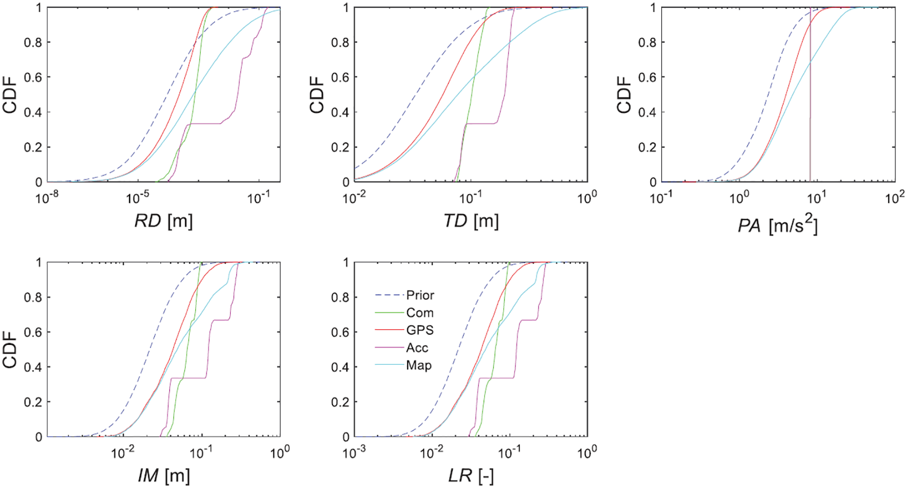
This subsection describes the results of the quantification of the uncertainty reduction for the two earthquake scenarios of Figure 6. In particular, Figure 9 illustrates the evolution of the estimates of η for the various parameters of interest with the number of samples drawn from scenario 1 (moderate earthquake). The results for PA when accelerometer observations are used are not shown because they are very high due to the low noise-to-signal ratio. It can be observed that 1000 samples are sufficient to achieve quite accurate estimates of this monitoring effectiveness measure based on pre-posterior variance analysis for all the parameters of interest. For the case of the loss ratio LR, characterized by higher values of η and a lower convergence rate, 2000 samples are required. Considering more samples would not significantly increase the accuracy of the estimates. With this number of samples, confident estimates of the values of the relative entropy measure D_KL can also be achieved for all the parameters of interest.

Figure 9.

Evolution with the number of samples of the monitoring effectiveness measure based on pre-posterior variance for the various parameters of interest and observation sources (scenario 1).

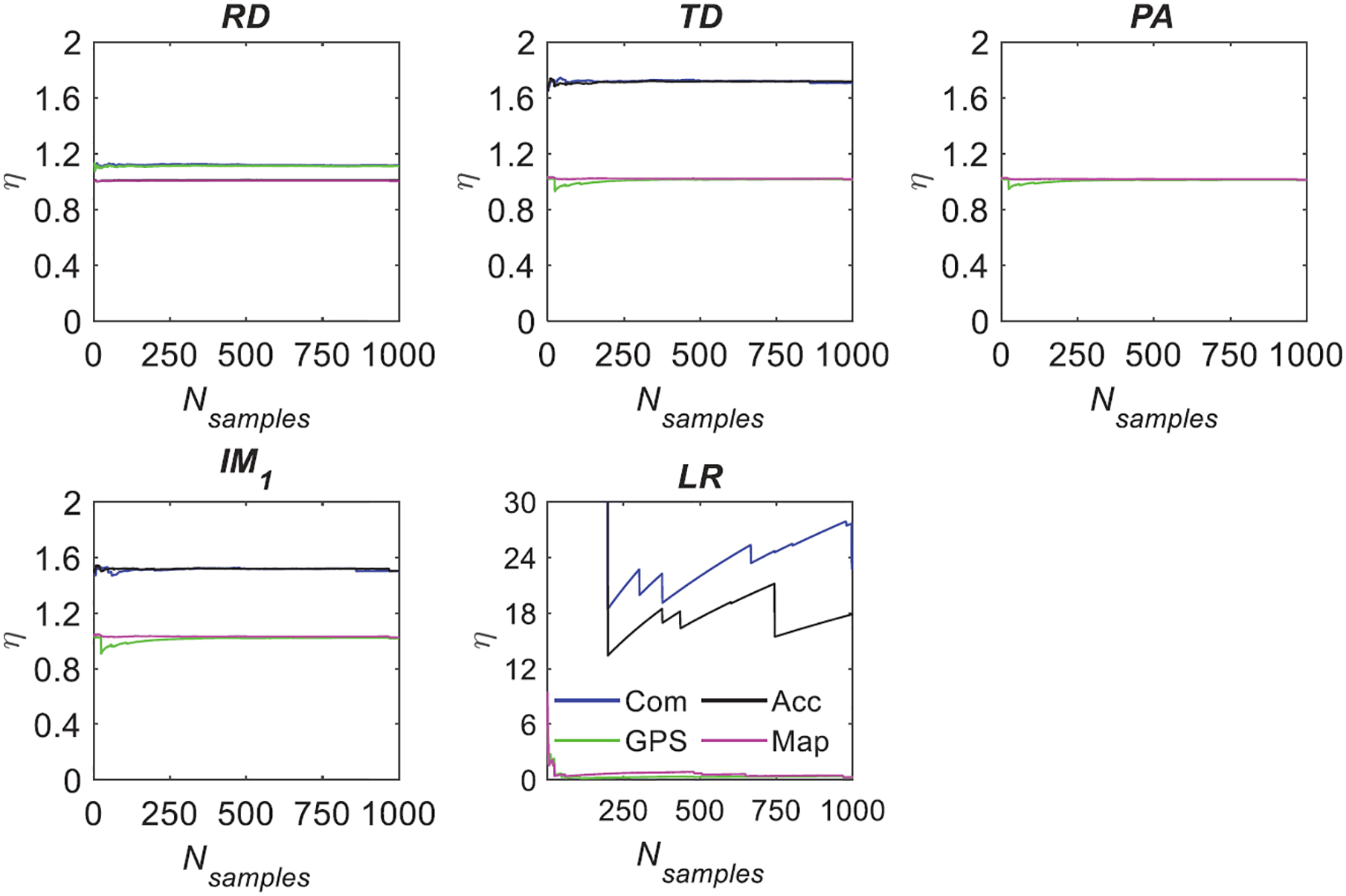
Tables 4 and 5 show the values of the effectiveness measures obtained based on the pre-posterior variance and the reduction of relative entropy for scenarios 1 and 2, respectively. These estimates of η and D_KL are based on 1000 samples in the case of all the parameters except LR, for which 2000 samples are used. With regard to the first measure of effectiveness, it can be observed that the values of η are all higher than 1 as expected, since adding information from sensors can only reduce uncertainty on average. For the same reason, the combined observations from multiple sensors result in a higher effectiveness, due to the lower variance of the parameters of interest compared to that obtained with a single sensor’s observation. GPSs are the most effective sensors for reducing the uncertainty in the residual drifts, and their effectiveness increases with the seismic intensity, since for low intensities the noise-to-signal ratio of the RD is high (the RDs are zero until the pier yields). Accelerometers are the most effective sensors for reducing the uncertainty of the PA, and also of the TD, given the significant correlation existing between PA and TD. The information from seismic stations located at reasonable distance from the site does not provide any benefit in terms of uncertainty reduction, given the low correlation existing between the IM at the site and that at the stations.

Table 4.

Pre-posterior variance-based effectiveness measure for estimation of various parameters of interest.

Scenario	M_w (–)	R (km)	Observation source	RD	TD	PA	IM	LR
1	5	30	Seismic stations (1)	1.002	1.015	1.011	1.025	1.000
			GPS (2)	1.110	1.012	1.000	1.017	1.000
			Accelerometer (3)	1.010	1.717	9.315	1.504	15.150
			Ground accelerometer (4)	1.003	1.982	1.507	28.020	4.575
			Combined (1,2,3)	1.120	1.730	9.327	1.524	15.150
			Combined (2,3,4)	1.124	2.321	10.009	28.280	42.580
2	6.5	20.7	Seismic stations (1)	1.000	1.000	1.000	1.000	1.000
			GPS (2)	1.344	1.055	1.008	1.017	1.086
			Accelerometer (3)	1.000	1.477	49.220	1.000	1.921
			Ground accelerometer (4)	1.277	1.869	2.164	316.160	1.305
			Combined (1,2,3)	1.428	2.305	49.220	1.026	2.348
			Combined (2,3,4)	1.579	3.531	50.430	317.826	2.250

RD: residual displacement; TD: peak transient displacement; PA: peak absolute acceleration; IM: intensity measure; LR: loss ratio; GPS: global positioning system.

Table 5.

Reduction of relative entropy-based effectiveness measure for estimation of various parameters of interest.

Scenario	M_w (–)	R (km)	Observation source	RD	TD	PA	IM	LR
1	5	30	Seismic station (1)	0.045	0.193	0.164	0.472	0.012
			GPS (2)	9.004	0.195	0.152	0.323	0.017
			Accelerometer (3)	0.121	28.261	182.464	18.838	0.200
			Ground accelerometer (4)	0.094	31.891	11.628	211.279	0.176
			Combined (1,2,3)	9.729	28.625	182.279	18.960	0.201
			Combined (2,3,4)	11.403	58.142	184.095	211.551	0.200
2	6.5	20.7	Seismic station (1)	0.374	1.217	1.259	5.415	0.073
			GPS (2)	31.771	8.794	6.296	12.151	0.139
			Accelerometer (3)	31.983	72.592	215.994	111.206	34.637
			Ground accelerometer (4)	4.126	27.991	41.805	220.421	4.067
			Combined (1,2,3)	51.566	119.331	216.049	112.024	36.688
			Combined (2,3,4)	62.447	132.049	214.224	220.441	32.072

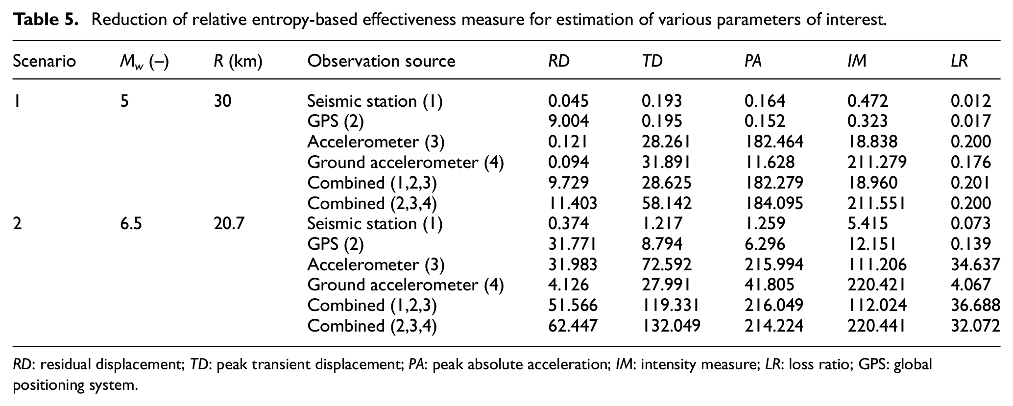
RD: residual displacement; TD: peak transient displacement; PA: peak absolute acceleration; IM: intensity measure; LR: loss ratio; GPS: global positioning system.

The reduction of uncertainty achieved for the losses is high in the case of low seismic intensity, and low for high seismic intensity. Moreover, in the case of low levels of shaking, sensors mounted on a structure can help to reduce the uncertainty in the estimation of the shaking intensity, and thus can be used to further improve ShakeMaps and achieve better estimates of the losses at structures not directly equipped with sensors. In the case of strong earthquakes, this effect of uncertainty reduction in the estimation of the IM is lost.

To shed further light on the reduction of uncertainty achievable with information on ground-shaking intensity, the case of a ground accelerometer placed at the base of the structure is also considered, providing an upper bound of the benefit in terms of uncertainty reduction derived from the use of ShakeMaps. It can be observed that if the seismic stations are located very close to the site, then the information they provide helps to reduce the uncertainty of the various parameters of interest. Similar observations were made in other studies,^89,90 indicating that a very dense network of seismometers in the vicinity of the site is required to obtain accurate estimates of the ground-motion intensity.

With regard to the second measure of the sensors’ effectiveness (D_KL), the observed trends are quite similar to those obtained for the first one, that is, the accelerometer mounted on the structure is the most effective for estimating displacements and accelerations, the GPS for the residuals, and higher effectiveness is achieved by combining more and more data. The reduction of uncertainty associated with ShakeMaps observations is quite low but slightly higher in the case of higher seismic intensities. This phenomenon is again explained by the distance from the two seismic stations to the bridge site (i.e. around a dozen kilometres), which is close to the spatial correlation distance of the Jayaram and Baker⁴⁷ model, that is, 15.9 km. As a result, the updates made to the values of the IM are much reduced, highlighting the need to deploy dense networks of seismic stations around exposed assets.

The only significant difference between the trends of the two effectiveness measures is for the LR estimates for scenario 1, characterized by high values of η for the accelerometer and combined observations, and generally low values of D_KL for all the observations. The opposite trend is observed for scenario 2. This discrepancy can be caused by the fact that the losses are generally very small, with a median value of 0 of the prior distribution. Moreover, in contrast to what is observed using the other effectiveness measurement, the reduction of uncertainty in the IM due to the observations is quite significant.

Conclusion and future work

This article illustrates a Bayesian framework for near real-time seismic damage assessment of critical structures that exploits heterogeneous sources of information from ShakeMaps, GPS receivers and accelerometers placed on the structure. Two alternative measures are proposed for quantifying the reduction of uncertainty from the observations, based on the concepts of pre-posterior variance and relative entropy reduction. The proposed framework is applied to investigate the effectiveness of the alternative sensing strategies for the rapid estimation of the response and the losses at a bridge under a moderate and a strong earthquake scenario.

Based on the observed results, the following conclusions can be drawn:

Among the sensors considered, the GPS sensor provides the best results in terms of uncertainty reduction when used to compute RDs of the piers, whereas the accelerometer placed at the top of the deck provides the best results in terms of reducing the uncertainty in the estimate of the absolute accelerations and drifts. The expected effectiveness of ShakeMaps is quite low, unless a seismic station is located very close to the structure.

The effectiveness of the sensors changes significantly with the shaking intensity. In the case of low shaking intensity, the effectiveness of the sensors in reducing the uncertainty is jeopardized by noise/measurement errors, particularly in the case of RDs. These errors become less significant in the case of high seismic shaking.

When the data from different sensors are combined together through the proposed BN, higher reductions of uncertainty are achieved as compared to when only single observation sources are considered separately.

The reduction of uncertainty in the losses can be very significant, whereas that in the estimate of the seismic shaking intensity is generally quite low.

The two measures of the monitoring effectiveness provide consistent results for most of the observed parameters and can be used interchangeably to quantify the reduction of uncertainty achievable with a monitoring strategy.

Future studies will address the quantification of the effectiveness of earthquake early warning techniques with a similar approach to that developed in this study and will also address alternative structural health monitoring schemes. Moreover, the proposed framework and results of these analyses will be used to develop a decision support system for bridges under extreme scenarios and to define optimal actions based on expected utility theory concepts. While the present study has demonstrated theoretical concepts on an arbitrary case study, further efforts within the TURNkey project (http://www.earthquake-turnkey.eu) may lead to an actual test and implementation of the approach, including the collection of real measurements.

Footnotes

Acknowledgements

We thank two anonymous reviewers for their detailed and insightful comments on an earlier version of this article.

Declaration of conflicting interests

The author(s) declared no potential conflicts of interest with respect to the research, authorship and/or publication of this article.

Funding

The author(s) disclosed receipt of the following financial support for the research, authorship and/or publication of this article: This paper was supported by the European Union’s Horizon 2020 research and innovation programme under grant agreement no 821046, project TURNkey (Towards more Earthquake-resilient Urban Societies through a Multi-sensor-based Information System enabling Earthquake Forecasting, Early Warning and Rapid Response actions). Input to and feedback on the draft manuscript by Dr Elisa Zuccolo at the European Centre for Training and Research in Earthquake Engineering (Eucentre), Italy, is greatly appreciated.

ORCID iDs

Enrico Tubaldi

Ekin Ozer

References

Erdik

Şeşetyan

Demircioğlu

, et al. Rapid earthquake loss assessment after damaging earthquakes. Soil Dyn Earthq Eng 2011; 31(2): 247–266.

Wald

Lin

Porter

, et al. ShakeCast: automating and improving the use of ShakeMap for post-earthquake decision-making and response. Earthq Spectra 2008; 24(2): 533–553.

Gehl

Douglas

D’Ayala

. Inferring earthquake ground-motion fields with Bayesian networks. B Seismol Soc Am 2017; 107(6): 2792–2808.

Michelini

Faenza

Lauciani

, et al. ShakeMap implementation in Italy. Seismol Res Lett 2008; 79(5): 688–697.

Bragato

. Assessing regional and site-dependent variability of ground motions for ShakeMap implementation in Italy. B Seismol Soc Am 2009; 99(5): 2950–2960.

Federal Emergency Management Agency (FEMA). HAZUS-MH MR1: technical manual (Volume earthquake model). Washington, DC: FEMA, 2003.

Lagomarsino

Cattari

Ottonelli

, et al. Earthquake damage assessment of masonry churches: proposal for rapid and detailed forms and derivation of empirical vulnerability curves. B Earthq Eng 2019; 17(6): 3327–3364.

Celebi

Sanli

Sinclair

, et al. Real-time seismic monitoring needs of a building owner – and the solution: a cooperative effort. Earthq Spectra 2004; 20(2): 333–346.

Limongelli

Omenzetter

Yazgan

, et al. Quantifying the value of monitoring for post-earthquake emergency management of bridges. In: Proceedings of the 39th IABSE symposium–engineering the future, Vancouver, BC, Canada, 21–23 September 2017.

10.

Soyoz

Feng

. Instantaneous damage detection of bridge structures and experimental verification. Struct Control Hlth 2008; 15(7): 958–973.

11.

. Recent research and applications of GPS based technology for bridge health monitoring. Sci China Technol Sci 2010; 53(10): 2597–2610.

12.

. Recent research and applications of GPS-based monitoring technology for high-rise structures. Struct Control Hlth 2013; 20(5): 649–670.

13.

Hurlebaus

Kang

. Summary review of GPS technology for structural health monitoring. J Struct Eng: ASCE 2013; 139(10): 1653–1664.

14.

Kaloop

Elbeltagi

, et al. Recent advances of structures monitoring and evaluation using GPS-time series monitoring systems: a review. ISPRS Int J Geo-Inf 2017; 6(12): 382.

15.

Porter

. A survey of bridge practitioners to relate damage to closure. Report no. EERL 2004-07, August 2004. Pasadena, CA: California Institute of Technology.

16.

Farrar

Worden

. An introduction to structural health monitoring. Philos T R Soc A 2007; 365(1851): 303–315.

17.

Reynders

Wursten

De Roeck

. Output-only structural health monitoring in changing environmental conditions by means of nonlinear system identification. Struct Health Monit 2014; 13(1): 82–93.

18.

Spencer

Jr Ruiz-Sandoval

Kurata

. Smart sensing technology: opportunities and challenges. Struct Control Hlth 2004; 11(4): 349–368.

19.

Ozer

. Multisensory smartphone applications in vibration-based structural health monitoring. Doctoral Dissertation, Columbia University, New York, 2016.

20.

Ozer

Feng

. Synthesizing spatiotemporally sparse smartphone sensor data for bridge modal identification. Smart Mater Struct 2016; 25(8): 085007.

21.

Ozer

Feng

. Direction-sensitive smart monitoring of structures using heterogeneous smartphone sensor data and coordinate system transformation. Smart Mater Struct 2017; 26(4): 045026.

22.

Ozer

Feng

. Hybrid motion sensing and experimental modal analysis using collocated smartphone camera and accelerometers. Meas Sci Technol 2017; 28(10): 105903.

23.

Douglas

Edwards

. Recent and future developments in earthquake ground motion estimation. Earth-Sci Rev 2016; 160: 203–219.

24.

Bommer

Crowley

. The influence of ground-motion variability in earthquake loss modelling. B Earthq Eng 2006; 4(3): 231–248.

25.

Park

Bazzurro

Baker

. Modeling spatial correlation of ground motion intensity measures for regional seismic hazard and portfolio loss estimation. In: Proceedings of the 10th international conference on applied statistics and probability, Tokyo, Japan, 31 July–3 August 2007.

26.

Crowley

Bommer

Stafford

. Recent developments in the treatment of ground-motion variability in earthquake loss models. J Earthq Eng 2008; 12(2): 71–80.

27.

Wald

Lin

Quitoriano

. Quantifying and qualifying USGS ShakeMap uncertainty. Reston, VA: United States Geological Survey, 2008, 26 pp.

28.

Porter

Mitrani-Reiser

Beck

. Near-real-time loss estimation for instrumented buildings. Struct Des Tall Spec 2006; 15(1): 3–20.

29.

Cremen

Baker

. Quantifying the benefits of building instruments to FEMA P-58 rapid post-earthquake damage and loss predictions. Eng Struct 2018; 176: 243–253.

30.

Hwang

Lignos

. Nonmodel-based framework for rapid seismic risk and loss assessment of instrumented steel buildings. Eng Struct 2018; 156: 417–432.

31.

Bayraktarli

Ulfkjaer

Yazgan

, et al. On the application of Bayesian probabilistic networks for earthquake risk management. In: Proceedings of the 9th international conference on structural safety and reliability (ICOSSAR 05), Rome, 19–23 June 2005, pp. 20–23.

32.

Bensi

. A Bayesian network methodology for infrastructure seismic risk assessment and decision support. Doctoral Dissertation, University of California, Berkeley, Berkeley, CA, 2010.

33.

Broglio

Crowley

Pinho

. Bayesian network framework for macro-scale seismic risk assessment and decision support for bridges. Pavia: IUSS Press, 2013.

34.

Gehl

. Bayesian networks for the multi-risk assessment of road infrastructure. Doctoral Dissertation, University College London (UCL), London, 2017.

35.

. Future of earthquake early warning: quantifying uncertainty and making fast automated decisions for applications. Doctoral Dissertation, California Institute of Technology, Pasadena, CA, 2014.

36.

Zonta

Glisic

Adriaenssens

. Value of information: impact of monitoring on decision-making. Struct Control Hlth 2014; 21(7): 1043–1056.

37.

Cappello

Zonta

Glišić

. Expected utility theory for monitoring-based decision-making. P IEEE 2016; 104(8): 1647–1661.

38.

Bolognani

Verzobio

Tonelli

, et al. IWSHM 2017: quantifying the benefit of structural health monitoring: what if the manager is not the owner? Struct Health Monit 2018; 17(6): 1393–1409.

39.

Pozzi

. What makes long-term monitoring convenient? A parametric analysis of value of information in infrastructure maintenance. Struct Control Hlth 2019; 26(5): e2329.

40.

Long

Döhler

Thöns

. Determination of structural and damage detection system influencing parameters on the value of information. Struct Health Monit. Epub ahead of print 24 January 2020. DOI: 10.1177/1475921719900918.

41.

Zonta

Cappello

Pozzi

, et al. On evaluating monitoring design effectiveness. In: Proceedings of the 7th European workshop on structural health monitoring (EWSHM’2014), Nantes, 8–11 July 2014.

42.

Thöns

. On the value of monitoring information for the structural integrity and risk management. Comput-Aided Civ Inf 2018; 33(1): 79–94.

43.

Limongelli

Giordano

. Vibration-based damage indicators: a comparison based on information entropy. J Civil Struct Health Monit 2020; 10: 251–266.

44.

Porter

. An overview of PEER’s performance-based earthquake engineering methodology. In: Proceedings of the 9th international conference on applications of statistics and probability in civil engineering, San Francisco, CA, 6–9 July 2003.

45.

Moehle

Deierlein

. A framework methodology for performance-based earthquake engineering. In: Proceedings of the 13th world conference on earthquake engineering, Vancouver, BC, Canada, 1–6 August 2004, paper no. 679.

46.

Schiappapietra

Douglas

. Modelling the spatial correlation of earthquake ground motion: insights from the literature, data from the 2016–2017 Central Italy earthquake sequence and ground-motion simulations. Earth-Sci Rev 2020; 203: 103139.

47.

Jayaram

Baker

. Correlation model for spatially distributed ground-motion intensities. Earthq Eng Struct D 2009; 38(15): 1687–1708.

48.

Scozzese

Tubaldi

Dall’Asta

. Assessment of the effectiveness of multiple-stripe analysis by using a stochastic earthquake input model. B Earthq Eng 2020; 18: 3167–3203.

49.

Vamvatsikos

Cornell

. Incremental dynamic analysis. Earthq Eng Struct D 2002; 31(3): 491–514.

50.

Mackie

Stojadinović

. Comparison of incremental dynamic, cloud, and stripe methods for computing probabilistic seismic demand models. In: Proceedings of the structures congress 2005: Metropolis and beyond, New York, 20–24 April 2005, pp. 1–11. Reston, VA: ASCE.

51.

Tubaldi

Freddi

Barbato

. Probabilistic seismic demand model for pounding risk assessment. Earthq Eng Struct D 2016; 45(11): 1743–1758.

52.

Freddi

Padgett

Dall’Asta

. Probabilistic seismic demand modeling of local level response parameters of an RC frame. B Earthq Eng 2017; 15(1): 1–23.

53.

Lemnitzer

Massone

Skolnik

, et al. Aftershock response of RC buildings in Santiago, Chile, succeeding the magnitude 8.8 Maule earthquake. Eng Struct 2014; 76: 324–338.

54.

Xie

Zhao

. Measuring the interstory drift of buildings by a smartphone using a feature point matching algorithm. Struct Control Hlth 2020; 27: e2492.

55.

Trapani

. A monitoring method for after-earthquake damage evaluation of buildings. Doctoral Dissertation, University of Trento, Trento, 2015.

56.

Çelebi

. GPS in dynamic monitoring of long-period structures. Soil Dyn Earthq Eng 2000; 20(5–8): 477–483.

57.

Dai

Wang

, et al. Use of residual drift for post-earthquake damage assessment of RC buildings. Eng Struct 2017; 147: 242–255.

58.

Ruiz-García

Chora

. Evaluation of approximate methods to estimate residual drift demands in steel framed buildings. Earthq Eng Struct D 2015; 44(15): 2837–2854.

59.

Goda

. Statistical modeling of joint probability distribution using copula: application to peak and permanent displacement seismic demands. Struct Saf 2010; 32(2): 112–123.

60.

Ruiz-García

Miranda

. Probabilistic estimation of residual drift demands for seismic assessment of multi-story framed buildings. Eng Struct 2010; 32(1): 11–20.

61.

Uma

Pampanin

Christopoulos

. Development of probabilistic framework for performance-based seismic assessment of structures considering residual deformations. J Earthq Eng 2010; 14(7): 1092–1111.

62.

Yazgan

Dazio

. Post-earthquake damage assessment using residual displacements. Earthq Eng Struct D 2012; 41(8): 1257–1276.

63.

Siringoringo

Fujino

. Lateral stability of vehicles crossing a bridge during an earthquake. J Bridge Eng 2018; 23(4): 04018012.

64.

Parvin

. The use of helical spring and fluid damper isolation systems for bridge structures subjected to vertical ground acceleration. Electron J Struct Eng 2001; 1(2): 98–110.

65.

Gkimprixis

Tubaldi

Douglas

. Evaluating alternative approaches for the seismic design of structures. B Earthq Eng 2020; 18: 4331–4361.

66.

Tubaldi

Barbato

Dall’Asta

. Transverse seismic response of continuous steel-concrete composite bridges exhibiting dual load path. Earthq Struct 2010; 1(1): 21–41.

67.

Tubaldi

Barbato

Dall’Asta

. Influence of model parameter uncertainty on seismic transverse response and vulnerability of steel–concrete composite bridges with dual load path. J Struct Eng: ASCE 2012; 138(3): 363–374.

68.

Zhang

Alam

. Performance-based seismic design of bridges: a global perspective and critical review of past, present and future directions. Struct Infrastruct E 2019; 15(4): 539–554.

69.

Choi

DesRoches

Nielson

. Seismic fragility of typical bridges in moderate seismic zones. Eng Struct 2004; 26(2): 187–199.

70.

Dutta

. On energy based seismic analysis and design of highway bridges. Doctoral Dissertation, The State University of New York at Buffalo, Buffalo, NY, 1999.

71.

Padgett

Dennemann

Ghosh

. Risk-based seismic life-cycle cost–benefit (LCC-B) analysis for bridge retrofit assessment. Struct Saf 2010; 32(3): 165–173.

72.

Basöz

Mander

. Enhancement of the highway transportation lifeline module in HAZUS. Washington, DC: National Institute of Building Sciences, 1999.

73.

Zeng

, et al. Improving the accuracy of near real-time seismic loss estimation using post-earthquake remote sensing images. Earthq Spectra 2018; 34(3): 1219–1245.

74.

Lunn

Spiegelhalter

Thomas

, et al. The BUGS project: evolution, critique and future directions (with discussion). Stat Med 2009; 28: 3049–3082.

75.

Kullback

Leibler

. On information and sufficiency. Ann Math Stat 1951; 22(1): 79–86.

76.

Gray

. Entropy and information theory. New York: Springer Science+Business Media, 2011.

77.

Dezi

. Architectural and structural design of short and medium span composite bridges. In: Proceedings of the 7th international conference on steel bridges, Guimarães, 4–6 June 2008.

78.

Tubaldi

Dall’Asta

Dezi

. Reduced formulation for post-elastic seismic response of dual load path bridges. Eng Struct 2013; 51: 178–187.

79.

EN 1994-2:2000. Eurocode 4: design of composite steel and concrete structures. Part 2: composite bridges (Brussels: European Committee for Standardization (CEN), 2000).

80.

McKenna

Fenves

Scott

. The open system for earthquake engineering simulation (OpenSees). Berkeley, CA: Pacific Earthquake Engineering Research Center, University of California, Berkeley, 2006.

81.

Scott

Fenves

. Plastic hinge integration methods for force-based beam–column elements. J Struct Eng: ASCE 2006; 132(2): 244–252.

82.

Baker

Lin

Shahi

, et al. New ground motion selection procedures and selected motions for the PEER transportation research program. PEER technical report 2011/03, January 2011. Berkeley, CA: Pacific Earthquake Engineering Research Center, University of California, Berkeley.

83.

Akkar

Bommer

. Empirical equations for the prediction of PGA, PGV, and spectral accelerations in Europe, the Mediterranean region, and the Middle East. Seismol Res Lett 2010; 81(2): 195–206.

84.

European Committee for Standardization (CEN) European Standard EN 1998-1:2005. Eurocode 8: design of structures for earthquake resistance. Part 1: general rules, seismic action and rules for buildings (Brussels: CEN, 2005).

85.

Trapani

Maroni

Debiasi

, et al. Uncertainty evaluation of after-earthquake damage detection strategy. In: Proceedings of the 2015 IEEE workshop on environmental, energy, and structural monitoring systems (EESMS), Trento, 9–10 July 2015, pp. 125–130. New York: IEEE.

86.

yetitmoves – Science for a Safer Land. DISPLAYCE: IoT solution for monitoring and early warning of displacements, 2020, http://yetitmoves.it/wp-content/uploads/2020/03/DISPLAYCE-en.pdf (accessed 12 October 2020).

87.

STMicroelectronics. LIS331DLH, https://www.st.com/en/mems-and-sensors/lis331dlh.html

88.

Woessner

Danciu

Kästli

, et al. Database of seismogenic zones, Mmax, earthquake activity rates, ground motion attenuation relations and associated logic trees. FP7 SHARE project deliverable D6.6, 2013, http://www.efehr.org/export/sites/efehr/.galleries/dwl_europe2013/D6-6_SHAREopt.pdf_2063069299.pdf

89.

Douglas

. Seismic network design to detect felt ground motions from induced seismicity. Soil Dyn Earthq Eng 2013; 48: 193–197.

90.

Ioannou

Douglas

Rossetto

. Assessing the impact of ground-motion variability and uncertainty on empirical fragility curves. Soil Dyn Earthq Eng 2015; 69: 83–92.