Development and validation of acoustic emission criteria for cracking assessment of prestressed RC girders

Abstract

The study presents a comprehensive analysis of acoustic emission (AE) data collected from bending tests on prestressed reinforced concrete (RC) girders, with the aim of detecting and characterizing cracking for structural health monitoring (SHM) applications. Multiple assessment approaches are implemented, including both established and newly developed AE-based criteria, organized into distinct method specifications (MSs). For each MS, novel damage classification rules are proposed, and blind predictions are carried out to identify damage states ranging from microcrack initiation to macrocrack formation. The performance of each method is quantitatively evaluated using precision, recall, accuracy, and a global score enabling a comparative assessment. Results show that several entropy-based MSs achieve high predictive performance, and optimum assessment criteria are experimentally calibrated. The correlation between AE activity and damage progression is validated using additional specimens not involved in the blind phase. The study demonstrates the feasibility of using AE parameters for reliable damage classification in RC girders and provides a validated framework to support SHM procedures and future field applications.

Keywords

Structural health monitoring (SHM)acoustic emission (AE)reinforced concrete (RC)damage criteria cracking

Introduction

The urgent need for early detection of damage in reinforced concrete (RC) and prestressed RC bridge members, with a focus on bridge girders,^1,2 has become evident, as recent structural failures have underscored the limitations of current structural health monitoring (SHM) approaches.^3,4 In particular, current SHM techniques, also considering experimental applications, still challengingly identify incipient and low-to-moderate damage in RC structures, especially referring to early microcracking initiation and evolution phenomena.⁵ Acoustic emission (AE) testing⁶ has emerged in the last few decades as a nondestructive testing technique with its capacity to potentially detect damage and degradation in real-time, automatically, and remotely,^7–9 over a wide range of materials and structures,^8,10–14 including prestressed structures.^2,15

Among the copious literature performing AE tests on RC elements, few studies provided quantitative damage assessment criteria and measures associated with prestressed girders, especially regarding post-tensioned systems. Abdelrahman et al.¹⁶ and ElBatanouny et al.¹⁷ tested prestressed beams under cyclic loading considering pre-cracked and corroded conditions. They developed a damage index based on cumulative energy and damage quantification charts, that is effective for identifying damage level and that would be promisingly applied for in situ monitoring. Omondi et al.¹⁸ combined AE testing and digital image correlation (DIC) to improve crack monitoring in prestressed RC sleepers, proving that AE-based assessment can be significantly more effective when DIC identifies the critical areas. Zeng et al.¹⁹ performed four-point bending tests on I-section prestressed beams, and implemented basic AE analysis to identify the evolution of the fracture process. The study provides potential damage descriptors based on acoustic activity that could be effective for monitoring in prestressed RC elements. Zhang et al.²⁰ tested prestressed girders by coupling AE testing to DIC and found that AE testing potentially detects crack earlier than traditional techniques and that it can significantly enhance accuracy of conventional monitoring techniques. Prem et al.²¹ identified AE energy versus deflection slope thresholds associated with formation on macrocracks in RC beams under bending, also correlating higher energy amounts to shear failure modes. The study characterized other correlations based on rise time to amplitude ratio (RA) versus average frequency (AF), severity index versus historic index, b-value (b_AE), but these were not supplied as quantitative assessment tools and only confirmed qualitative trends or failure modes.

Elbatanouny et al.²² carried out bending tests on prestressed bridge girders removed from real bridges and developed intensity analysis charts that would be efficient for early detection of cracking deterioration. Castellanos-Toro et al.¹⁵ tested posttensioned beams under both static and vibration loading conditions, reproducing the evolution from precracking to macrocrack. They identified potential acoustic damage correlations but confirmed the challenging data interpretation, also highlighting that limited information regarding current state and previous loading history of the structure might harden the damage interpretation.

Overall, AE testing showed potential correlations with mechanical response and damage evolution, but no studies, to the authors’ knowledge, focused on incipient and low-to-moderate cracking damage identification, systematically investigated multiple analysis methods, and provided robust damage criteria (DC), for example, by means of unbiased assessment or blind predictions (BPs). Moreover, literature correlations and criteria often reflect specific material and structural applications and can be difficult to extend to different scenarios. Thus, a pressing need exists for a thorough investigation that rigorously and quantitatively assesses current AE-based evaluation methods, potentially introducing new method specifications (MSs) and criteria as tools to detect early and low-to-moderate damage in typical prestressed girders.

The present study covers the abovementioned literature gap by systematically evaluating the effectiveness of various AE analysis methods in detecting early-stage and moderately developed cracking damage in prestressed RC girders. To this end, the study employed a comprehensive experimental program, integrating blind AE monitoring with mechanical and visual damage assessments to establish reference damage states (DSs). The novelty and scientific contribution of the paper refers to (1) methodological novelty, by implementing an AE testing framework integrated with BP and introducing revised and new MSs, (2) quantitative evaluation, by defining promising DC and objectively assessing their performance across multiple methods, and (3) practical relevance, by demonstrating how the proposed criteria could be employed for proof-testing and SHM of real-world bridge elements.

Experimental tests

Mechanical tests

Six posttensioned RC girder specimens were tested under four-point bending in the framework of an extensive experimental campaign aimed at assessing the influence of different grouting conditions, prestressed levels, and strengthening techniques on flexural response.^1,23 Four tests, namely on specimens S1, S2, S3, and S4, represent the main core of the study, whereas two additional tests on specimens S5 and S6 were carried out for validation purposes; these latter tests are described in section “Validation considering additional specimens.”

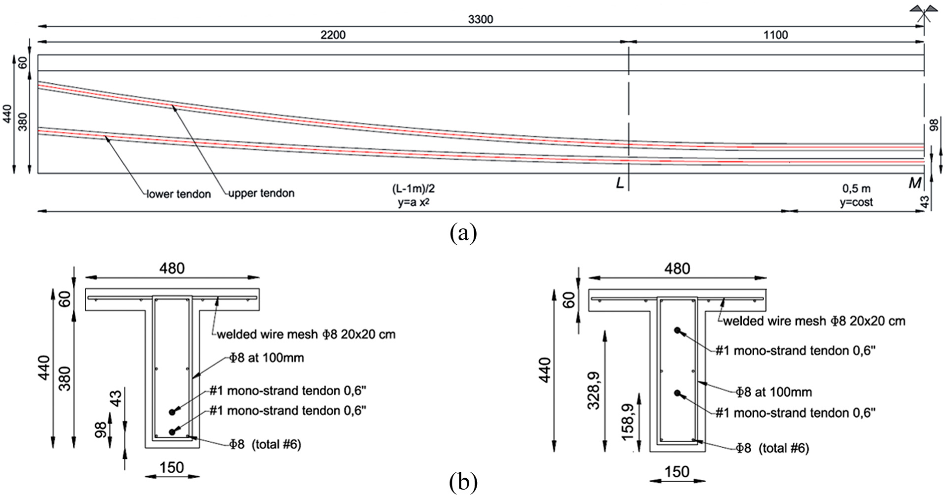
The girder geometry was designed as representative of a real bridge deck with longitudinal beams having T-cross section in a length scale of 1:5. The internal posttensioning system resulted in two parabolic monostrand tendons with different prestress levels among different girders (Figure 1).

Figure 1.

Unstrengthened (benchmark) specimen: (a) longitudinal view and (b) midspan (left) and end (right) cross section of the girder specimen (dimensions in mm).^1,23

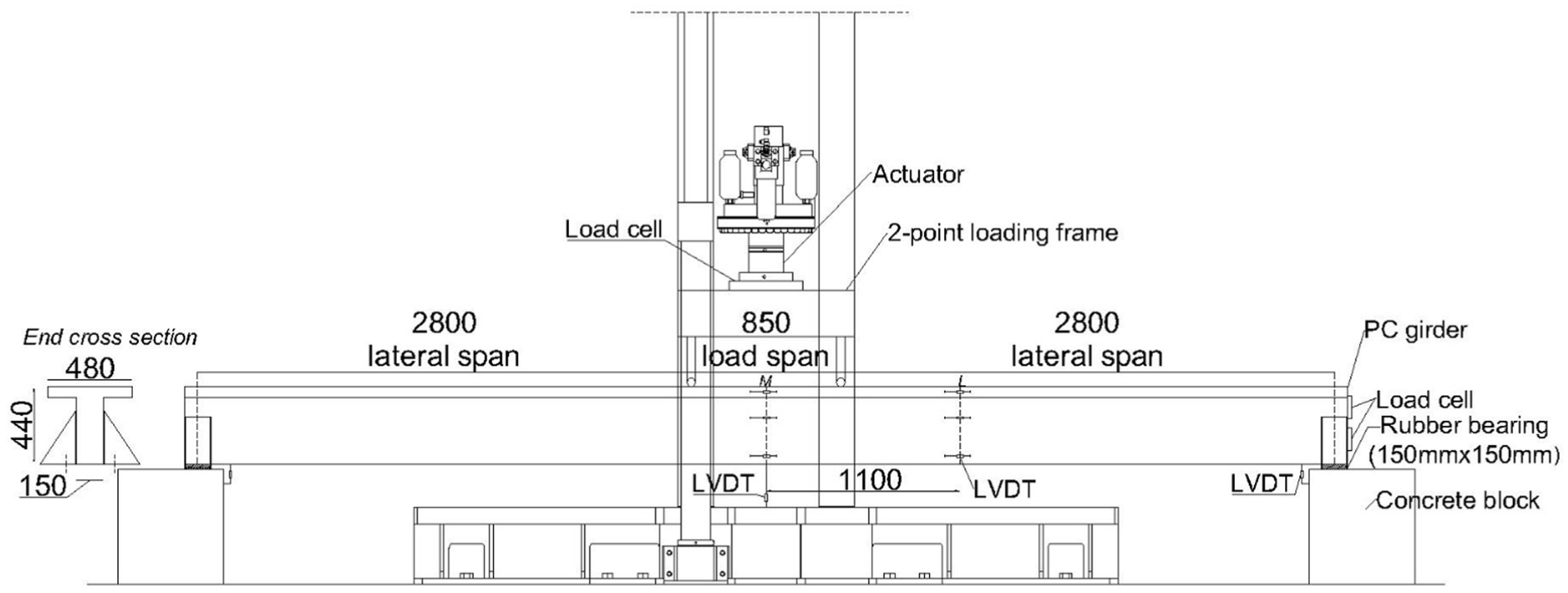
The tests were conducted at the Department of Structures for Engineering and Architecture of the University of Naples Federico II, the experimental layout with the specimen beam is reported in Figure 2. The testing program consisted into a sequence of two loading protocols, as follows: protocol P1, which consisted of a force-controlled quasi-static cyclic test in accordance with ACI 437²⁴; and protocol P2, which was a displacement-controlled monotonic test untill (P2). Three subprotocols were defined within P1, namely P1L1, P1L2, and P1L3, aimed at providing three different external force levels (F_e) with increasing amplitude corresponding to F_e,1, F_e,2, F_e,3; each P1 protocol consists in two equal-peak force cycles. These force levels were associated with serviceability limit state (F_e,1), ultimate limit state (F_e,2), and 1.5 times amplified ultimate limit state (F_e,3), resulting in 33.1, 48.3, and 72.4 kN, respectively, as discussed in Losanno et al.²³ and depicted in Figure 3. After completing P1, a quasi-static monotonic protocol untill failure (P2) was imposed with a displacement rate of 0.05 mm/s up to either the beam collapse or the peak stroke (150 mm) of the actuator whatever reached first.

Figure 2.

Four-point bending testing setup (dimensions in mm).^1,23

Figure 3.

P1L1, P1L2, and P1L3 loading protocols expressed as applied force (F_e) versus time (t).²³

The applied force F_e was measured through a load cell installed between the actuator head and the loading frame, whilst midspan deflection was measured through a linear variable differential transducer and a wire potentiometer.

Acoustic emission (AE) tests

AE tests were performed with the multichannel AMSY-6 system produced by Vallen Systeme (Bürgermeister-Seidl-Str., Deutschland) using the acquisition software Visual AE. Nonintegrated and preamplified piezoelectric sensors were used, that is, VS30 and VS150 sensors, working in 28–80 kHz and 100–450 kHz, and resonant at 30 and 150 kHz, respectively. Specifically, only VS30 sensors were used for testing S1 specimen, whereas only VS150 ones were used for testing S3 and S4; to correlate VS30 and VS150 responses, S2 was tested with both VS30 and VS150. These two types of sensors were used to assess the AE sensitivity in terms of low (VS30) and medium (VS150) frequency resonance/operation, given that AE testing of RC structures is typically carried out within this range.^15,17 Validation tests, performed on S5 and S6, also implemented sensors with intermediate working/resonant frequencies (VS75), as described in section “Validation considering additional specimens.”

Four sensor channels were implemented for each test, and typically three sensors were located in the middle point area. In particular, for specimen S1 and all loading protocols but P1L1, Ch1, Ch2, and Ch4 sensors were located in the middle point area (28 cm away from middle point axis), and Ch3 was out of this latter area (178 cm away from middle point axis); Ch4 was in the support area (located 278 cm away from middle point axis) under P1L1 test. For other specimens, Ch1, Ch2, and Ch3 sensors were located in the middle point area (28 cm away from middle point axis), and Ch4 was out of the area (approximately 90–100 cm away from middle point axis).

Pretrigger and posttrigger time interval was set equal to 100 μs, hit definition time, hit lockout time, and maximum hit duration time were set equal to 250 μs, 2000 μs, and 100 ms, respectively; no peak definition time was set. Band-pass 25–82 and 75–350 kHz filters were implemented for VS30 and VS150 sensors, respectively. Gain was set to 34 dB and input setting to 10 Vpp.

Check and preparation tests were carried out to verify the installation of the sensors and to calibrate the main acquisition parameters; pencil-lead break, pulsing tests, and sensors’ localization tests were performed. Only recordings along the mechanical tests were analyzed in this study; in particular, AE data were identified by channel (Ch1, Ch2, Ch3, and Ch4) and related mechanical test, that is, specimen (S1, S2, S3, and S4) and loading protocol (P1L1, P1L2, P1L3, and P2). All basic AE features were recorded, with a focus on number of hits or hits (H), peak amplitude or amplitude (A), number of counts (N), rise time (RT), duration (D), energy (E), root mean square (RMS), signal strength (SS), cumulative hits (ΣH), cumulative counts (ΣN), and cumulative energy (ΣE). As a postprocessing filter, N >3 was assumed.

Damage assessment criteria and blind predictions (BPs)

Methodology

AE analysis and MSs

Four different methods (Ms)/analysis parameters were considered: Kaiser effect (and Felicity ratio), RA versus AF response, b-value, and acoustic entropy, implemented considering multiple MSs; the formulations are omitted since are described in the reference papers, and the only developed MSs are reported.

Violation of Kaiser effect²⁵ and associated Felicity ratio (FR)²⁶ were assessed (method (M) K) considering a number of 11 MSs, depending on the quantitative definition of significant activity descriptors, that is, considering:

hits (H) versus time (t) rate (ΔH/Δt) larger than or equal to 3/s, defining MS K1;

counts (N) larger than or equal to 100 (MS K2.1);

hits (H) larger than or equal to 10 and amplitude (A) larger than or equal to 60 dB, (MS K2.2);

history index larger than or equal to 1.4, considering four different formulations, applied considering the case of resetting and not resetting N and the correlation factor, defining MSs K3.1a, K3.1b, K3.2a, K3.2b, K3.3a, K3.3b, K3.4a, K3.4b, where index i in K.3i corresponds to the MS identifier (ID) and following a or b stands for resetting or not resetting condition, respectively. M K was assessed considering each cycle of the cyclic tests (but the first unprogrammed cycle of P1L1) and monotonic tests.

Only a MS was implemented for RA versus AF (or AFRA) analysis,²⁷ assessing the evolution of RA versus AF for all channels and over subsequent subsets within each test (MS AFRA).

b-value (b_AE; method (M) b)²⁸ was estimated considering the same subsets considered for AFRA analysis, considering both current data and accumulated data, defining MS b1 and MS b2, respectively.

Finally, AE or acoustic (information) entropy (H)^29,30 (M E) was assessed considering both (E1) Shannon (H_S) and (E2) Kullback–Leibler (H_KL) formulations,^31,32 and accounting for both (1) (H_S and H_KL) absolute and (2) cumulative (ΣH_S and ΣH_KL) measures, defining MS E1.1, E1.2, E2.1, and E2.2. H_S and H_KL formulations are reported in Equations (1) and (2), respectively, considering the Jth AE event, and the probability distribution mass vector p_J is expressed in Equation (3), where N_i is the number of counts associated with the ith AE event (numerator ith items).

H_{S} (J) = - \sum_{j = 1}^{J} p_{J} (j) \log_{2} (p_{J} (j))

(1)

\begin{matrix} H_{KL} (J) = H_{S} (p_{J} (j) | p_{J} (j - 1)) \\ = - \sum_{j = 2}^{J} p_{J} (j) \log_{2} (\frac{p_{J} (j)}{p_{J} (j - 1)}) \end{matrix}

(2)

p_{J} = \frac{1}{\sum_{i = 1}^{J} N_{i}} {N_{1}, N_{2}, \dots, N_{J}}

(3)

Entropy was assessed starting from the first AE event and increasing detection window along time including each consequent AE event.

Damage assessment

The assessment methodology is organized in four steps: (1) M selection, (2) M implementation (through MS), (3) AEs processing according to MS, and (4) damage assessment results. Figure 4 shows the workflow considering M K and MS K1 as an example.

Figure 4.

Workflow of the implemented assessment methodology (Table 1). P2 is analyzed up to a peak force of 1.5 times P1L3 peak force (1.5 F_e,3).

AEs processing (step 3) is based on the implementation of quantitative DC, defined for each method and MS as it is reported in Table 1. Each implementation of DC yielded a BP (step 4), which consists in a DS corresponding to each specimen and loading protocol.

Table 1.

Damage assessment methodology: DC associated with implemented assessment methods and MSs: DC ID, EC, DSWs, and DSC.

	DC
					DSW	DSC
MS ID	DC ID	EC				ND	LD	SD
K1	K1	EC:Kaiser effect is violated (FR <1)			Each cycle of P1 tests and P2 up to peak force of 1.5 times P1L3 is a DSW	No channel detects EC	Only one channeldetects EC	More thanone channeldetects EC
K2.1	K2.1
K2.2	K2.2
K3.1a	K3.1a
K3.1b	K3.1b
K3.2a	K3.2a
K3.2b	K3.2b
K3.3a	K3.3a
K3.3b	K3.3b
K3.4a	K3.4a
K3.4b	K3.4b
AFRA	AFRA	EC:AF decreasesand RA increases simultaneously atconsequent subsets			Each test isdivided in six DSW (subsets)	Less than two EC detectionsover all channels	More than oneand less than four EC detections over all channels	More thanthree EC detectionsover allchannels
b1	b1.1	EC:b_AE decreases atconsequent steps
	b1.2	EC:b_AE≤1
b2	b2.1	EC:b_AE decreases atconsequent steps
	b2.2	EC:b_AE≤1
E1.1	E1.1	EC₁:H_S < 5 bits	EC₂:5 ≤H_s< 10 bits	EC₃:H_S≥ 10 bits	Each test is a DSW	No channel detectsEC₃ and less than three channels detect EC₂	Only one channeldetects EC₃ ormore than twochannels detect EC₂	More thanone channelsdetect EC₃
E1.2	E1.2	EC₁:ΣH_S < 10² bits	EC₂:10² ≤ΣH_S < 10⁴	EC₃:ΣH_S≥ 10⁴ bits
E2.1	E2.1	EC₁:H_KL < 0.25 bits	EC₂:0.25 ≤ H_KL< 0.50 bits	EC₃:H_KL≥ 0.50 bits
E2.2	E2.2	EC₁:ΣH_KL < 5 bits	EC₂:5 ≤ ΣH_KL< 10 bits	EC₃:ΣH_KL≥ 10 bits

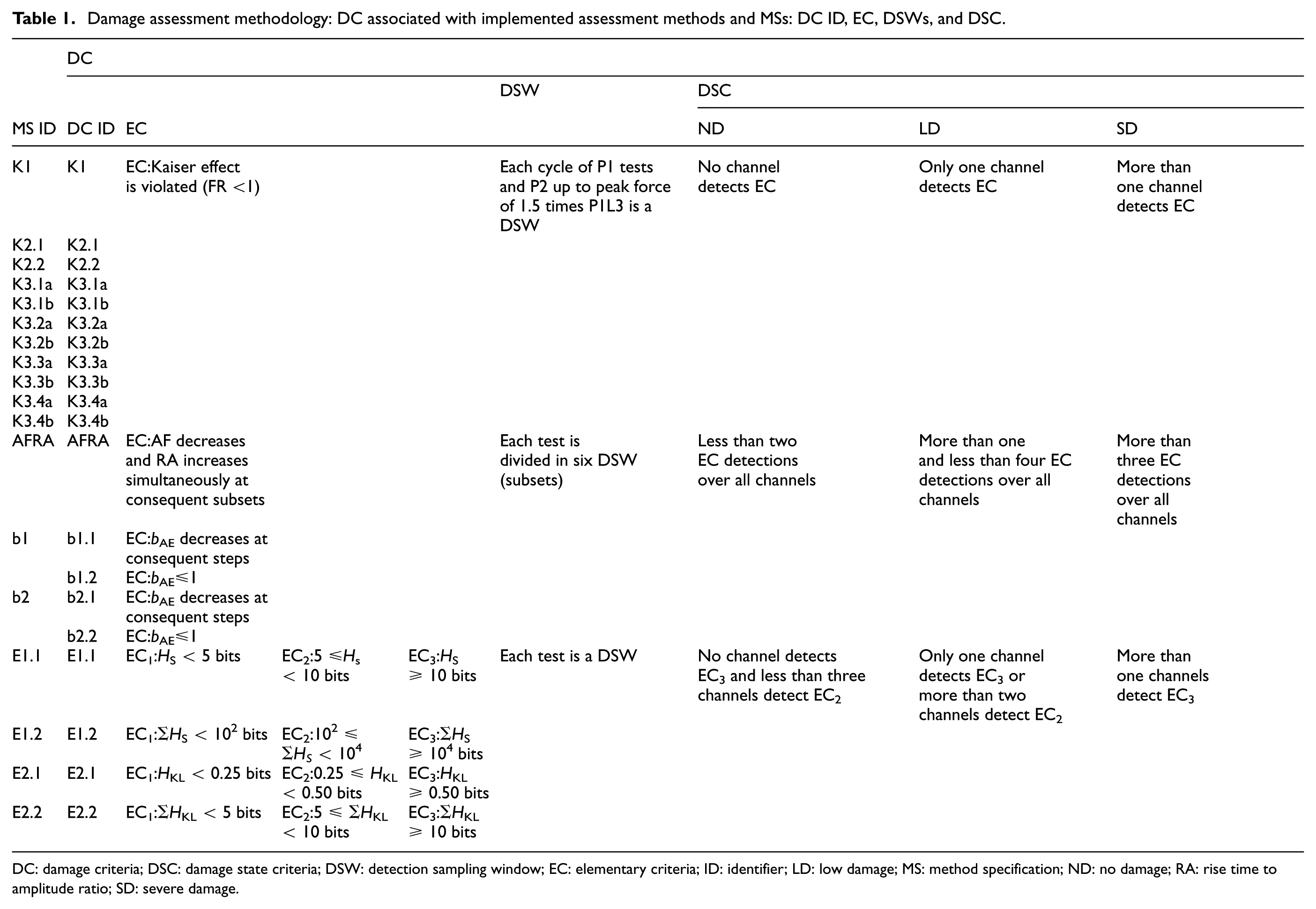
DC: damage criteria; DSC: damage state criteria; DSW: detection sampling window; EC: elementary criteria; ID: identifier; LD: low damage; MS: method specification; ND: no damage; RA: rise time to amplitude ratio; SD: severe damage.

DC were defined by a set of rules and analysis features implemented by processing the results associated with each MS. Each DC is defined by DC ID, elementary criteria (EC), detection sampling windows (DSWs), and damage state criteria (DSC). DC IDs correspond to MS IDs unless multiple DC are defined for a single MS. EC correspond to elementary detections referred to the specific conditions (e.g., violation of Kaiser effect or entropy threshold exceedance) checked in DSWs, identified within each loading protocol. For a given DC ID, the quantitative interpretation of the EC detections over the sensor channels results in a DSC, which allows to define a BP.

EC define the level of attention associated with the specific detection, and binary or ternary EC were defined according to the specific DC. Binary EC are based non-EC detection (null level of attention) and EC detection (low to severe level of attention); ternary EC are associated with EC₁ (null level of attention), EC₂ (low-to-moderate level of attention), and EC₃ (moderate-to-severe level of attention). EC (Table 1) were defined according to the interpretation of the AE results and accounting for the literature evidence.

EC associated with K, AFRA, and b MSs were set considering well consolidated DC. With regard to E MSs, EC₃ were derived from the blind criteria already considered for the analysis of the results, whereas EC₁ and EC₂ were defined by setting (1) half EC₃ as a reference EC₁/EC₂ threshold value for E1.1, E2.1, and E2.2, which operate in the context of a single order of magnitude and (2) 10⁻² EC₃ as a reference EC₁/EC₂ threshold value for E1.2.

For fixed sensor channels, DSWs (Table 1) represent the context of the assessment realization associated with EC checks. DSWs associated with investigated MSs coincide with related subsets. In detail, DSWs related to the Kaiser effect and Felicity ratio MSs (K MSs) consist in each cycle of P1 tests and to P2 up to peak force of 1.5 times P1L3. DSWs related to AFRA and b-value analysis MSs coincide with the following set of six subsets For P1L1, subsets include (1) first and second increasing (loading) branches of first cycle, (2) third and fourth increasing branches of first cycle, (3) fifth and sixth increasing branches of first cycle, (4) (all) first cycle decreasing branches, (5) (all) second cycle increasing branches, and (6) (all) second cycle decreasing branches. For P1L2 and P1L3, subsets include (1) first increasing (loading) branch of first cycle, (2) second and third increasing branches of first cycle, (3) fourth and fifth increasing branches of first cycle, (4) (all) first cycle decreasing branches, (5) (all) second cycle increasing branches, and (6) (all) second cycle decreasing branches. For P2, subsets were defined by considering a number of six equal-time windows up to the achievement of a force equal to 1.5 times the maximum force associated with P1L3 (F_e,3). DSW related to the acoustic entropy MSs coincide with the entire test.

DSC (Table 1) define specific rules for interpreting, in a univocal quantitative manner, the results of EC checks within DSW for each MS (and specimen). DSC essentially consist in criteria associated with number and level of attention of detected EC over total number of channels and DSWs. DSC are defined for three hypothesized DSs, classified among no damage (ND), low damage (LD), and severe damage (SD), for each specimen and loading protocol. Since the predictions are blind, the classification of the level of damage is based on reasonable clear distinguishable criteria, which also account for the range of observed parameter/feature values. Obviously, DSC were quantitatively defined with regard to the specific tests, but these can be easily extended to other applications by referring to the size of DSWs and accounting for the number of sensor channels.

For each MS, the synthesis of the application of DSC to all loading protocols and specimens provides a BP. In particular, a BP is expressed by a 4 × 4 matrix, where rows represent loading protocols (P1L1, P1L2, P1L3, and P2) and columns stand for specimens (S1, S2, S3, and S4). P2 was considered up to a peak force of 1.5 times P1L3 peak force (1.5 F_e,3) in order to not account for extremely severe loading conditions (e.g., near collapse).

In order to account for the dispersion of the investigated DC in terms of BP matrices, mode (M-matrix), disagreement frequency (DF-matrix), and entropy (E-matrix) were estimated. M-matrix was defined by the most frequently predicted DS, DF-matrix corresponded to the frequency of deviation from the mode, and E-matrix was defined by Shannon entropy (H_S), associated with different DSs considering the ratio between the DS detection counts and the number of estimations; ND, LD, and SD corresponded to 1, 2, and 3, respectively.

Results and discussion remarks

Key response occurrences

The experimental results are processed in this article identifying the key response occurrences, considering Kaiser effect and Felicity ratio, AFRA, b_AE, and acoustic entropy.

The occurrence of Kaiser violations reported in Table 2 clearly indicates that specimen S1 and S2 were affected by damage since protocol P1L1, with more (less) significant damage associated with S1 (S2) as 5 (2) occurrences were detected; a number of 5 occurrences is detected for S2 corresponding to P1L2. A number of 3 and 1 occurrences associated with S3 and S4, respectively, were observed corresponding to P1L3, and, corresponding to P2, the occurrences associated with S4 become more significant (4). Once again, the number and significance of the Kaiser effect violations potentially indicates the evolution of damage.

Table 2.

Sum of total occurrences of Kaiser effect violation along cycles (cycles 1 and 2 for protocols P1 and unique test procedure for protocol P2) for each test and specimen, considering all channels (MS K3.1b).

Kaiser effect violation	S1	S2	S3	S4
Protocol
P1L1	5	2	0	0
P1L2	7	5	0	0
P1L3	7	8	3	1
P2	4	4	3	4
Total P1	19	15	3	1

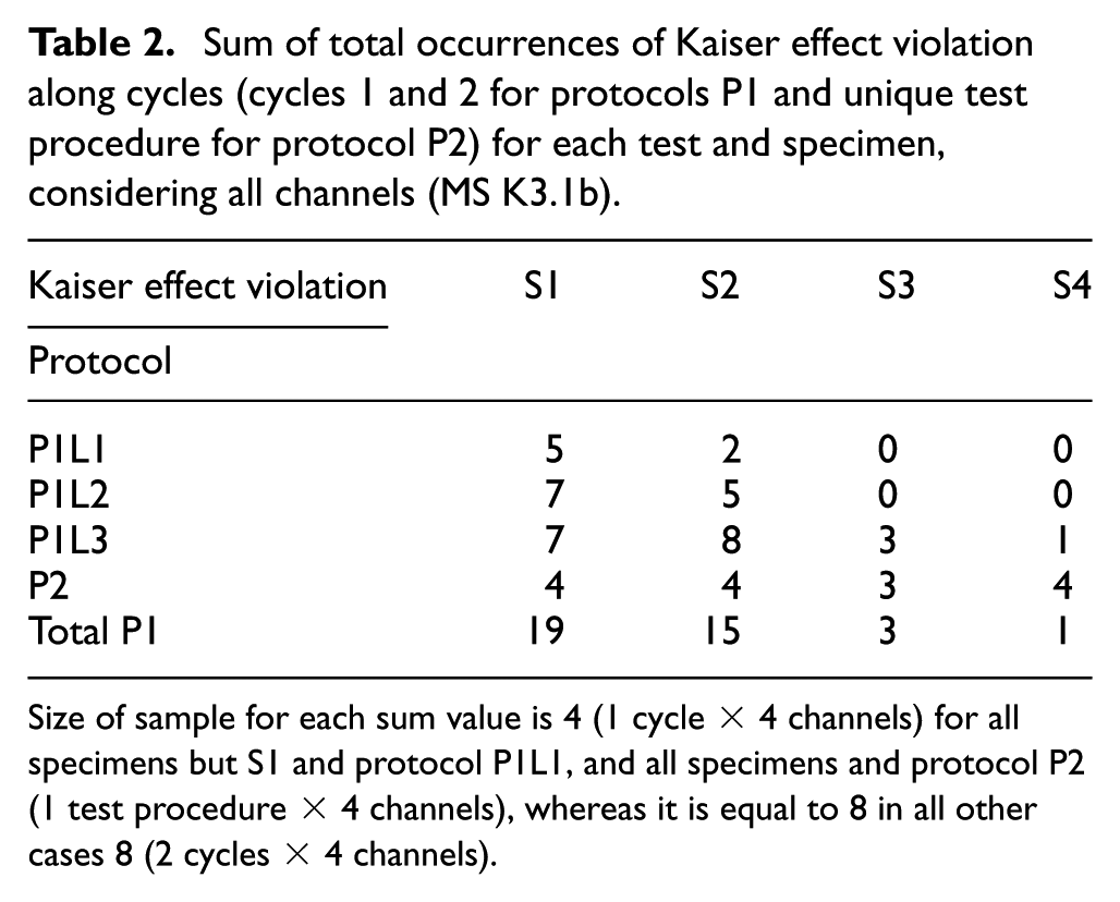
Size of sample for each sum value is 4 (1 cycle × 4 channels) for all specimens but S1 and protocol P1L1, and all specimens and protocol P2 (1 test procedure × 4 channels), whereas it is equal to 8 in all other cases 8 (2 cycles × 4 channels).

Tables 3 –6 report the cases in which AF decreases and RA increases simultaneously for specimens S1, S2, S3, and S4, respectively, for each test and channel. A summary of total occurrences is reported in Table 3.

Table 3.

Simultaneous occurrences (1/0) of decreasing AF and increasing RA along subsequent subsets for each test and channel, associated with specimen S1 (MS AFRA).

AF decreasing andRA increasingoccurrences (1/0)	S1
	Subset 1–2				Subset 2–3				Subset 3–4				Subset 4–5				Subset 5–6
Protocol	ch 1	ch 2	ch 3	ch 4	ch 1	ch 2	ch 3	ch 4	ch 1	ch 2	ch 3	ch 4	ch 1	ch 2	ch 3	ch 4	ch 1	ch 2	ch 3	ch 4
P1L1	0	1	0	0	1	1	0	0	1	0	0	0	0	0	1	0	1	0	0	0
P1L2	0	0	0	0	1	0	0	1	0	0	0	0	1	0	0	1	0	0	0	0
P1L3	0	1	0	1	0	0	0	1	0	0	0	0	1	1	1	1	0	0	0	0
P2	1	0	0	1	0	0	1	1	0	0	1	0	0	1	1	0	0	0	1	0

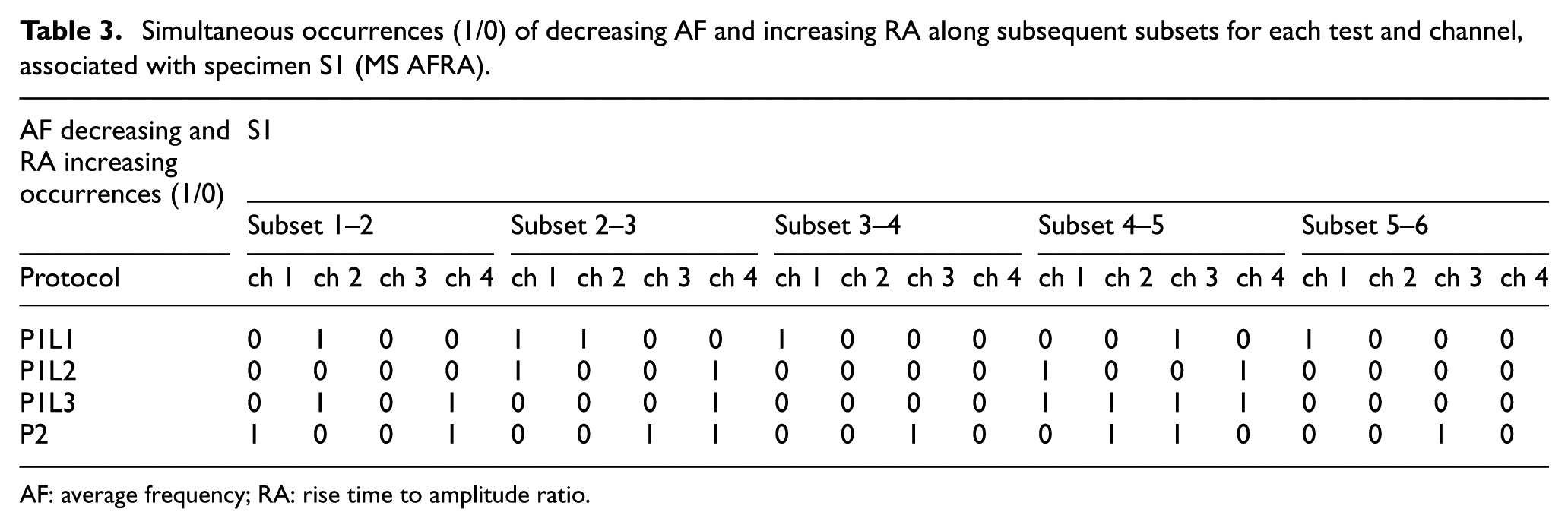
AF: average frequency; RA: rise time to amplitude ratio.

Table 4.

Simultaneous occurrences (1/0) of decreasing AF and increasing RA along subsequent subsets for each test and channel, associated with specimen S2 (MS AFRA).

AF decreasing andRA increasingoccurrences (1/0)	S2
	Subset 1–2				Subset 2–3				Subset 3–4				Subset 4–5				Subset 5–6
Protocol	ch 1	ch 2	ch 3	ch 4	ch 1	ch 2	ch 3	ch 4	ch 1	ch 2	ch 3	ch 4	ch 1	ch 2	ch 3	ch 4	ch 1	ch 2	ch 3	ch 4
P1L1	1	1	1	0	0	1	0	0	1	0	0	0	1	0	0	0	1	1	1	0
P1L2	1	0	0	0	1	0	0	0	0	0	1	0	1	1	0	0	1	0	0	0
P1L3	0	1	0	0	0	0	0	0	1	1	1	1	0	0	0	0	0	1	0	0
P2	0	1	1	0	0	0	1	1	0	0	0	0	0	0	0	0	0	1	1	0

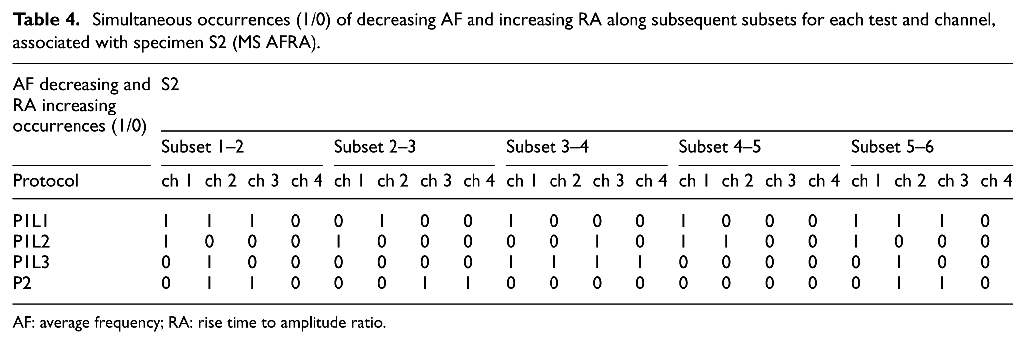
AF: average frequency; RA: rise time to amplitude ratio.

Table 5.

Simultaneous occurrences (1/0) of decreasing AF and increasing RA along subsequent subsets for each test and channel, associated with specimen S3 (MS AFRA).

AF decreasing andRA increasingoccurrences (1/0)	S3
	Subset 1–2				Subset 2–3				Subset 3–4				Subset 4–5				Subset 5–6
Protocol	ch 1	ch 2	ch 3	ch 4	ch 1	ch 2	ch 3	ch 4	ch 1	ch 2	ch 3	ch 4	ch 1	ch 2	ch 3	ch 4	ch 1	ch 2	ch 3	ch 4
P1L1	0	0	0	0	0	0	0	0	0	0	0	0	0	0	0	0	0	0	0	0
P1L2	0	0	0	0	0	0	0	0	0	0	0	0	0	0	0	0	0	0	0	0
P1L3	0	0	0	0	0	0	0	0	0	0	0	0	1	0	1	1	0	0	0	0
P2	0	1	0	0	1	0	0	0	0	1	0	0	1	0	0	1	0	0	0	1

AF: average frequency; RA: rise time to amplitude ratio.

Table 6.

Simultaneous occurrences (1/0) of decreasing AF and increasing RA along subsequent subsets for each test and channel, associated with specimen S4 (MS AFRA).

AF decreasing andRA increasingoccurrences (1/0)	S4
	Subset 1–2				Subset 2–3				Subset 3–4				Subset 4–5				Subset 5–6
Protocol	ch 1	ch 2	ch 3	ch 4	ch 1	ch 2	ch 3	ch 4	ch 1	ch 2	ch 3	ch 4	ch 1	ch 2	ch 3	ch 4	ch 1	ch 2	ch 3	ch 4
P1L1	0	0	0	0	0	1	0	0	0	0	0	0	0	0	0	0	0	0	0	0
P1L2	0	0	0	0	0	0	0	0	0	0	0	0	0	0	0	0	0	0	0	0
P1L3	0	0	0	0	0	0	0	0	0	0	0	0	0	0	0	0	0	0	0	0
P2	0	0	0	0	0	0	1	0	0	0	1	0	1	0	1	0	0	0	0	1

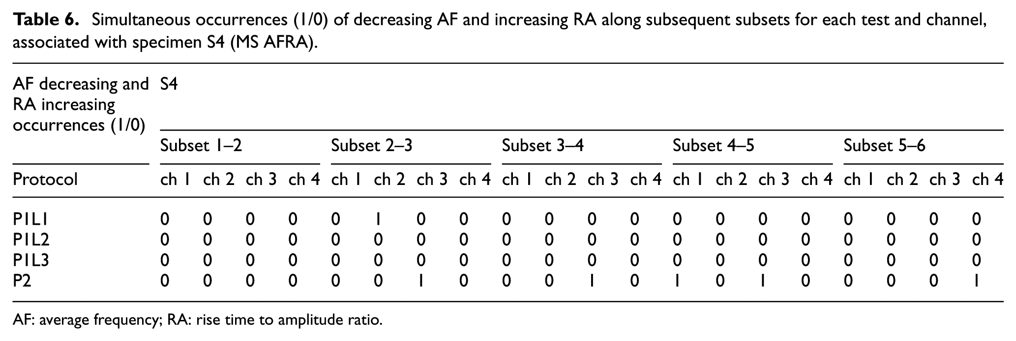
AF: average frequency; RA: rise time to amplitude ratio.

Table 7 considers all channels. According to the total occurrences, S1 and S2 were significantly affected by P1L1, whereas null to one occurrence were associated with S3 and S4. The number of occurrences decreases passing from P1L1 to P1L2 for S1 and S2, with no occurrences related to S3 and S4 under P1L2. P1L3 occurrences related to S1 and S2 are comparable with P1L1 and P1L2 ones, whereas a number of three and zero occurrences are detected for S3 and S4, respectively. Finally, occurrences related to S1 and S2 increase from P1L3 to P2, and a significant number of occurrences also affect S3 and S4. The abovementioned detections suggest that S1 and S2 might be affected by damage since P1L1, whereas, only from P1L3 and P2, S3 and S4 begin to be damaged, respectively. It is recalled that P2 data are associated with the detection windows that extend up to 1.5 F_e,3.

Table 7.

Summary of total simultaneous occurrences of decreasing AF and increasing RA along subsequent subsets for each test and specimen, considering all channels (MS AFRA).

Total AF decreasing and RA increasing occurrences	S1	S2	S3	S4
Protocol
P1L1	6	8	0	1
P1L2	4	5	0	0
P1L3	7	5	3	0
P2	8	6	6	5
Total P1	17	18	3	1

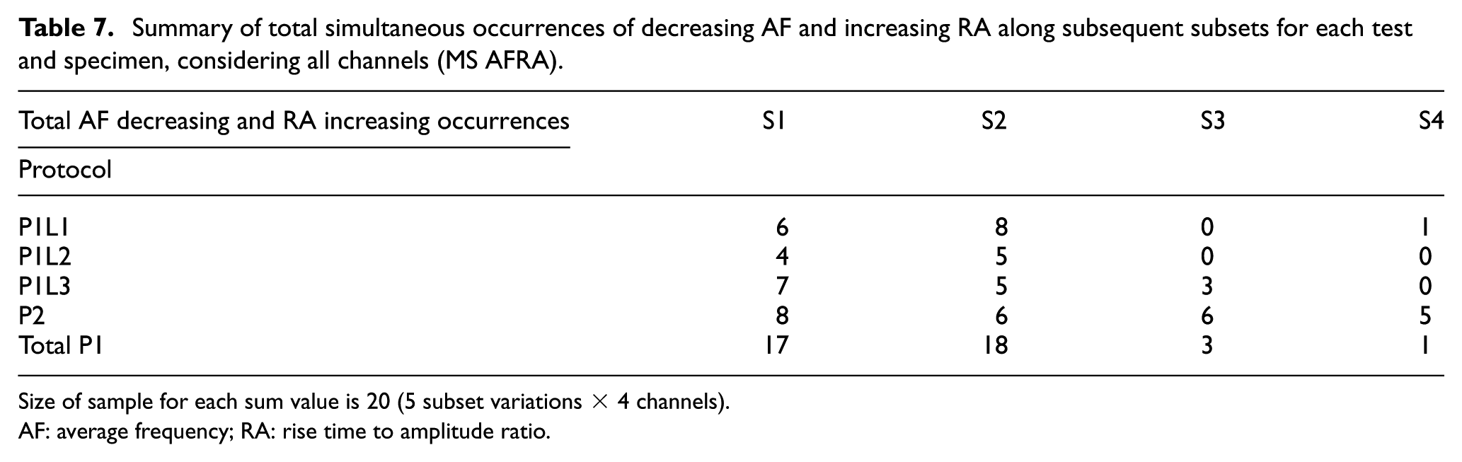
Size of sample for each sum value is 20 (5 subset variations × 4 channels).

AF: average frequency; RA: rise time to amplitude ratio.

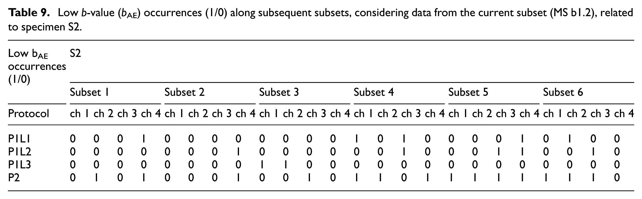
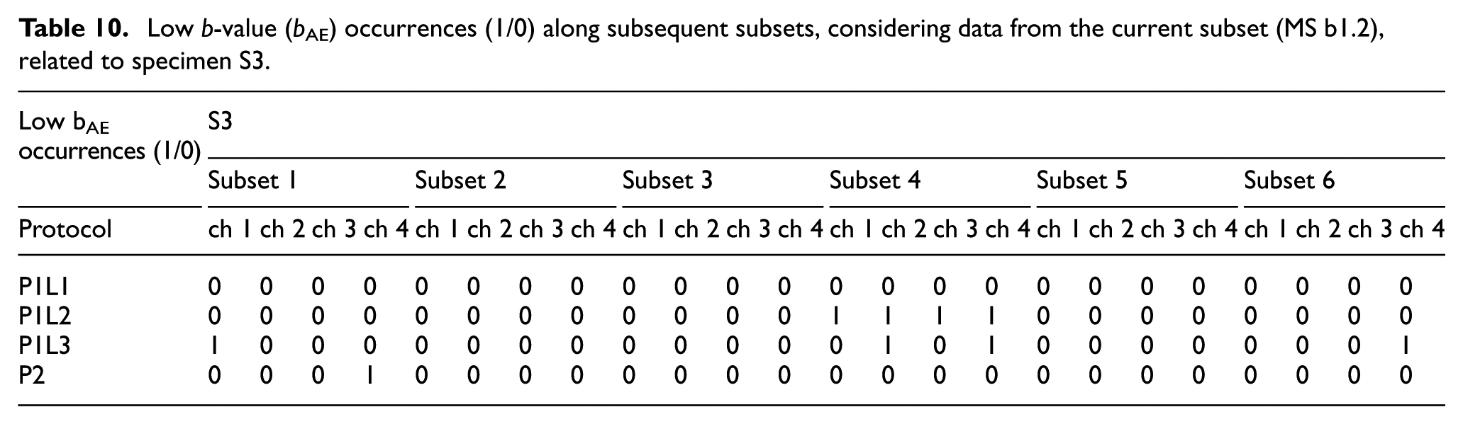
As a representative result of b-value assessment, MS b1.2 occurrences are depicted in Tables 8 –11, and a summary of the abovementioned results is reported in Table 12 considering both MS b1 and MS b2, accounting for all channels. As a general trend, it can be noted that all MSs identify more significant occurrences for S1 and S2, with minor but not negligible occurrences corresponding to S3 and S4. More significant occurrences associated with S3 and S4 are detected under P1L2 or P1L3, and, unexpectedly, decreasing occurrences related to P2 are almost negligible for S3 and S4, whereas low occurrence ones are more consistent with preceding protocols and other specimens. Table 12 shows similar trends identified with regard to previous analysis methods, but it yields less clear evidence regarding the hypothetical damage initiation regarding S3 and S4. Nevertheless, b-value was already known to not be necessarily well correlated with damage developing in complex structures and components, especially under complex stress-strain fields (Soltangharaei et al.³³).

Table 8.

Low b-value (b_AE) occurrences (1/0) along subsequent subsets, considering data from the current subset (MS b1.2), related to specimen S1.

Low b_AEoccurrences(1/0)	S1
	Subset 1				Subset 2				Subset 3				Subset 4				Subset 5				Subset 6
Protocol	ch 1	ch 2	ch 3	ch 4	ch 1	ch 2	ch 3	ch 4	ch 1	ch 2	ch 3	ch 4	ch 1	ch 2	ch 3	ch 4	ch 1	ch 2	ch 3	ch 4	ch 1	ch 2	ch 3	ch 4
P1L1	1	1	1	1	0	0	0	0	0	0	0	0	0	0	1	1	0	0	0	0	0	0	0	0
P1L2	0	0	0	0	0	0	1	0	1	1	1	0	0	1	1	0	0	1	0	0	0	1	1	0
P1L3	0	1	0	0	0	1	0	0	1	1	0	1	1	1	1	0	1	1	0	0	1	1	0	0
P2	0	0	0	0	0	0	0	0	1	1	0	1	1	1	0	1	1	1	1	1	1	1	1	1

Table 9.

Low b-value (b_AE) occurrences (1/0) along subsequent subsets, considering data from the current subset (MS b1.2), related to specimen S2.

Low b_AEoccurrences(1/0)	S2
	Subset 1				Subset 2				Subset 3				Subset 4				Subset 5				Subset 6
Protocol	ch 1	ch 2	ch 3	ch 4	ch 1	ch 2	ch 3	ch 4	ch 1	ch 2	ch 3	ch 4	ch 1	ch 2	ch 3	ch 4	ch 1	ch 2	ch 3	ch 4	ch 1	ch 2	ch 3	ch 4
P1L1	0	0	0	1	0	0	0	0	0	0	0	0	1	0	1	0	0	0	0	1	0	1	0	0
P1L2	0	0	0	0	0	0	0	1	0	0	0	0	0	0	1	0	0	0	1	1	0	0	1	0
P1L3	0	0	0	0	0	0	0	0	1	1	0	0	0	0	0	0	0	0	0	0	0	0	0	0
P2	0	1	0	1	0	0	0	1	0	0	1	0	1	1	0	1	1	1	1	1	1	1	1	0

Table 10.

Low b-value (b_AE) occurrences (1/0) along subsequent subsets, considering data from the current subset (MS b1.2), related to specimen S3.

Low b_AEoccurrences (1/0)	S3
	Subset 1				Subset 2				Subset 3				Subset 4				Subset 5				Subset 6
Protocol	ch 1	ch 2	ch 3	ch 4	ch 1	ch 2	ch 3	ch 4	ch 1	ch 2	ch 3	ch 4	ch 1	ch 2	ch 3	ch 4	ch 1	ch 2	ch 3	ch 4	ch 1	ch 2	ch 3	ch 4
P1L1	0	0	0	0	0	0	0	0	0	0	0	0	0	0	0	0	0	0	0	0	0	0	0	0
P1L2	0	0	0	0	0	0	0	0	0	0	0	0	1	1	1	1	0	0	0	0	0	0	0	0
P1L3	1	0	0	0	0	0	0	0	0	0	0	0	0	1	0	1	0	0	0	0	0	0	0	1
P2	0	0	0	1	0	0	0	0	0	0	0	0	0	0	0	0	0	0	0	0	0	0	0	0

Table 11.

Low b-value (b_AE) occurrences (1/0) along subsequent subsets, considering data from the current subset (MS b1.2), related to specimen S4.

Low b_AEoccurrences(1/0)	S4
	Subset 1				Subset 2				Subset 3				Subset 4				Subset 5				Subset 6
Protocol	ch 1	ch 2	ch 3	ch 4	ch 1	ch 2	ch 3	ch 4	ch 1	ch 2	ch 3	ch 4	ch 1	ch 2	ch 3	ch 4	ch 1	ch 2	ch 3	ch 4	ch 1	ch 2	ch 3	ch 4
P1L1	0	0	0	1	0	0	1	0	1	0	0	0	0	1	0	0	0	1	0	0	0	0	0	0
P1L2	0	0	0	0	0	0	0	0	0	0	0	1	0	0	0	0	0	0	0	0	0	0	0	0
P1L3	0	0	0	0	0	0	0	0	0	0	1	1	1	1	0	0	0	1	0	0	1	0	0	0
P2	0	0	0	0	0	0	1	0	0	0	0	0	0	0	0	0	0	0	0	0	0	0	0	0

Table 12.

Summary of total low b-value (b_AE) and decreasing value occurrences subsequent subsets considering data from the current subset (MS b1) and cumulative data (MS b2) for each test and specimen, considering all channels.

Total low or decreasingb_AE occurrences	MS b1								MS b2
	Low				Decreasing				Low				Decreasing
Protocol	S1	S2	S3	S4	S1	S2	S3	S4	S1	S2	S3	S4	S1	S2	S3	S4
P1L1	6	9	0	3	6	5	0	5	2	4	1	1	7	2	0	1
P1L2	5	5	4	0	9	5	4	1	5	4	5	2	10	1	6	4
P1L3	9	7	5	4	12	2	4	6	7	3	2	1	11	3	2	8
P2	16	12	12	8	14	14	1	1	18	11	8	7	14	12	1	1
Total P1	20	21	9	7	27	12	8	12	14	11	8	4	28	6	8	13

Size of sample for each sum value is 24 (6 subsets variations × 4 channels) and 20 (5 subsets × 4 channels) for low value occurrences and decreasing occurrences, respectively.

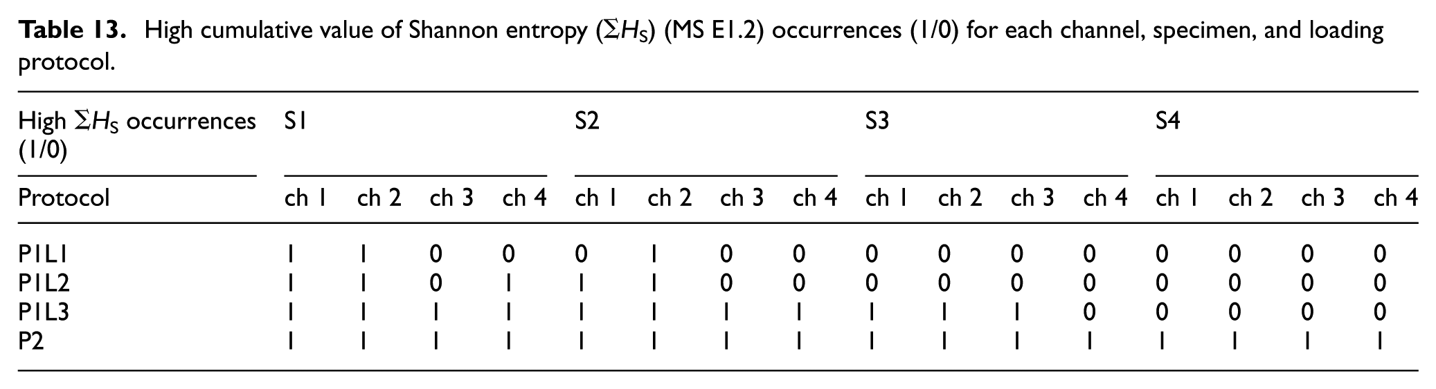
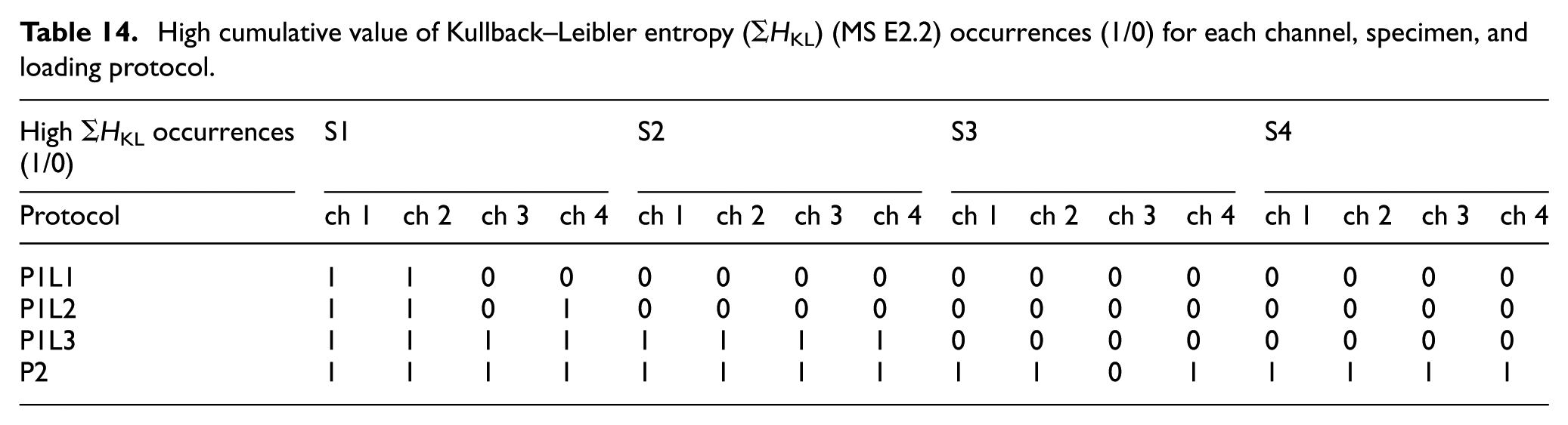
Acoustic entropy was estimated considering the same subsets considered for AF versus RA and b-value analysis, but the focus of the assessment was on the maximum entropy values within each test. In particular, the occurrences of high values associated with ΣH_S (MS E1.2) and ΣH_KL (MS E2.2) are presented in Tables 13 and 14, and a summary associated with all investigated entropy measures is reported in Table 15. At this stage of the BP, high entropy threshold values related to H_S, ΣH_S, H_KL, and ΣH_KL were set equal to 10, 10⁴, 0.5, and 10, respectively, according to data observations but also accounting for past applications.

Table 13.

High cumulative value of Shannon entropy (ΣH_S) (MS E1.2) occurrences (1/0) for each channel, specimen, and loading protocol.

High ΣH_S occurrences (1/0)	S1				S2				S3				S4
Protocol	ch 1	ch 2	ch 3	ch 4	ch 1	ch 2	ch 3	ch 4	ch 1	ch 2	ch 3	ch 4	ch 1	ch 2	ch 3	ch 4
P1L1	1	1	0	0	0	1	0	0	0	0	0	0	0	0	0	0
P1L2	1	1	0	1	1	1	0	0	0	0	0	0	0	0	0	0
P1L3	1	1	1	1	1	1	1	1	1	1	1	0	0	0	0	0
P2	1	1	1	1	1	1	1	1	1	1	1	1	1	1	1	1

Table 14.

High cumulative value of Kullback–Leibler entropy (ΣH_KL) (MS E2.2) occurrences (1/0) for each channel, specimen, and loading protocol.

High ΣH_KL occurrences(1/0)	S1				S2				S3				S4
Protocol	ch 1	ch 2	ch 3	ch 4	ch 1	ch 2	ch 3	ch 4	ch 1	ch 2	ch 3	ch 4	ch 1	ch 2	ch 3	ch 4
P1L1	1	1	0	0	0	0	0	0	0	0	0	0	0	0	0	0
P1L2	1	1	0	1	0	0	0	0	0	0	0	0	0	0	0	0
P1L3	1	1	1	1	1	1	1	1	0	0	0	0	0	0	0	0
P2	1	1	1	1	1	1	1	1	1	1	0	1	1	1	1	1

Table 15.

Summary of total occurrences of high value of investigated entropy measures (MS E1.1, MS E1.2, MS E2.1, and MS E2.2) for each test and specimen, considering all channels.

Total high entropy occurrences	MS E1.1				MS E1.2				MS E2.1				MS E2.2
Protocol	S1	S2	S3	S4	S1	S2	S3	S4	S1	S2	S3	S4	S1	S2	S3	S4
P1L1	2	1	0	0	2	1	0	0	3	3	2	3	2	0	0	0
P1L2	3	2	0	0	3	2	0	0	2	1	3	2	3	0	0	0
P1L3	4	4	0	0	4	4	3	0	1	2	3	2	4	4	0	0
P2	4	4	4	4	4	4	4	4	1	3	2	2	4	4	3	4
Total P1	9	7	0	0	9	7	3	0	6	6	8	7	9	4	0	0

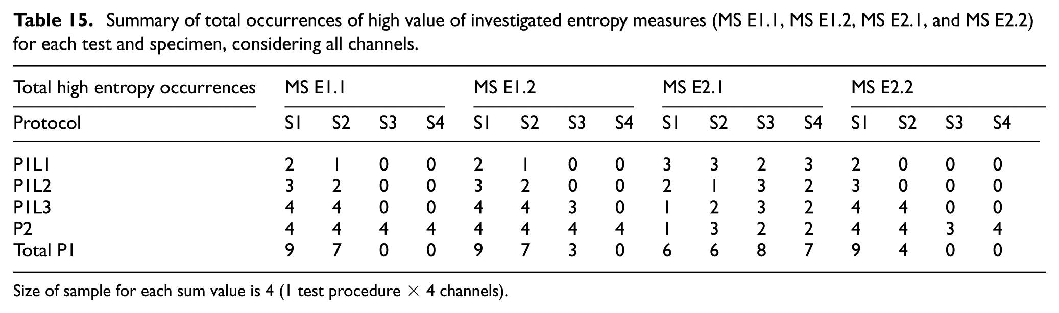
Size of sample for each sum value is 4 (1 test procedure × 4 channels).

Blind predictions (BPs)

Figure 5(a) depicts all BPs associated with investigated DC. All BPs tend to detect an increasing severity damage trend passing from protocol P1L1 to P2 and a decreasing one from S1 to S4, with a combination of these effects when both features vary. There are clear similarities among the different estimations, for example, in most cases, ND was associated with P1L1 for S1 and S2 specimens, whereas in most cases, SD was detected for all specimens under P2 test. Outlier BPs are associated with b-value-based estimations (MS b) and with entropy-based prediction corresponding to Kullback–Leibler entropy (MS E.2.1). This latter prediction is extremely severe for all protocol-specimen combinations (SD is detected in 13 cases out of 16), differently from all other BPs.

Figure 5.

Damage assessment results: (a) BP matrices corresponding to estimated DSs associated with investigated protocols and specimens for all DC and (b) Dispersion analysis of BPs: M-matrix, DF-matrix, and E-matrix. M-matrix values 1, 2, and 3 correspond to ND, LD, and SD, respectively; DF-matrix values are associated with estimation deviances from the mode; E-matrix values report Shannon entropy measures, considering ND, LD, and SD corresponding to 1, 2, and 3, respectively.

Figure 5(b) shows the results of the dispersion analysis. M-matrix estimation highlights the most frequent DS associated with the set of investigated DC, and this represents a measure of consensus among the different BPs. The experimental interpretation of M-matrix is crucial since all predictions are blind and several different methods and formulations were implemented to derive BPs; this is reported in the following section. For S1 and S2, all protocol mode estimates are associated with SD, as well as P2 estimates associated with all specimens; for S3 and S4, ND is associated with P1L1–P1L2 and P1L1–P1L2–P1L3, respectively, whereas LD is only frequently estimated for S3 under P1L3. It is interesting to note that LD condition, representing a transition between LD and SD, only appears 1 time out of 16 cases in M-matrix, and this suggests that this mechanical state is more difficultly detected.

DF-matrix depicts how often the estimations disagree (deviations from the mode), and high values are associated with significant variability. Looking at the M-matrix as a reference, highest DF-matrix counts are overall associated with first DS achievements or DS transitions, and this is meaningful since the earliest achievement of DS is certainly the most challenging condition to assess. In particular, a deviation value equal to 11 corresponds to specimen S2 under P1L1 (first test) and a value equal to 12 is related to the transition between LD and SD.

Finally, E-matrix represents a quantitative measure of uncertainty and disorder, and, in this context, it indicates how much the different estimations are spread across multiple DSs. E-matrix could be evaluated considering acceptable entropy thresholds potentially associated with reasonably uncertain and disordered estimations, according to the case study DS. Further comments are omitted since this matrix, as well as the other ones, will be meaningfully interpreted with regard to the disclosed experimental data in the following section.

Experimental assessment of blind predictions (BPs)

Experimental response and damage states (DSs)

Figure 6 depicts the applied force (F_e) versus deflection (Δ) curves associated with all specimens and loading protocols. The primary focus of this experimental assessment was on identifying DSs related to the observed cracking initiation and evolution process, defined by ND, LD, and SD. Therefore, the mechanical response of the specimens is not discussed in detail, and only the conventional identification of DSs is highlighted in this paper.

Figure 6.

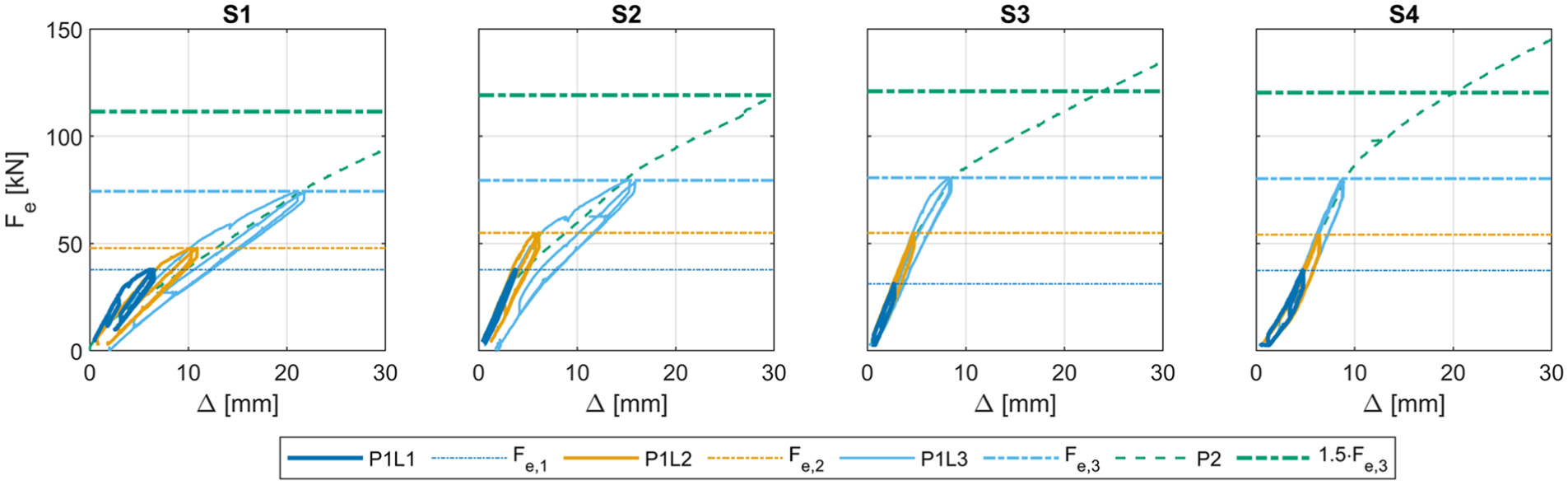
Applied force (F_e) versus deflection (Δ) curves associated with specimens S1, S2, S3, and S4 and related protocol force limits.

Even if nominal concrete properties were kept constant for all specimens providing an average cubic strength of 35 MPa after 28 days of curing, the specimens were designed with a different prestress level. Specifically, the target prestress jacking forces in Table 16 were applied to the specimens through both internal and external posttensioning (S3 and S4 only).

Table 16.

Prestress applied to specimens: internal (P_int), external (P_ext), and total (P_tot) prestress jacking force.

Specimen	P _int [kN]	P _ext [kN]	P _tot [kN]
S1	150	0	150
S2	300	0	300
S3	300	100	400
S4	150	250	400

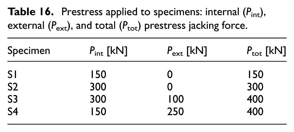
The different prestressing levels resulted in significantly different damage scenarios for the specimens. In detail, S1 was designed to develop cracking under external load lower than F_e,1, thus representing the behavior of an existing bridge with low residual prestress. Prestress level in S2 was considered representative of bridges in fair conditions, which may not cause cracking under service traffic loads. In S3 and S4, an additional posttensioning system aimed at improving the flexural capacity of the girders under both service and ultimate loads considering different internal prestress levels.

The object of interest for the present assessment is the mechanical phase that initiates with the tensile microcracking formation, which might not even be visible, corresponding to the earliest visible deviation from linear elastic response (incipient reduction of flexural stiffness from the initial conditions), and ends with the evolution of macrocracking that affects, in a considerable and steady manner, the flexural stiffness (postcracked cross-section stiffness), namely a steady stiffness reduction larger than 20%. In this study, the former phase is conventionally referred to as LD, whereas the latter to SD. The transition phase can be relatively gradual and not straightforward to identify, especially in terms of damage initiation. LD and SD were identified by synthesizing physical observations (cracks noted during testing, especially for SD) and force-deflection response data.²³ Even though the analysis of the crack patterns is beyond the scope of this article, an example of crack pattern typically associated with SD is illustrated in Figure 7. It can be noted that the crack is just visible, and it extends from the bottom surface to over 10 cm, with a width exceeding 0.1 mm in the lower crack portion tending to decrease along the evolution. LD condition is associated with microcracks that are not generally visible for their extremely reduced width and extension.

Figure 7.

Example of crack pattern associated with achievement of conventional SD state.

The achievement of SD can be clearly observed in Figure 6: global significant stiffness degradation due to macrocracking associated with specimens S1, S2, S3, and S4 can be associated with P1L1, P1L3, P2, and P2, respectively, recalling that in these latter two cases SD is identified between F_e,3 and 1.5 F_e,3, as this latter force threshold was considered in the damage assessment previously discussed. SD conditions were clearly compatible with the damage pattern (macrocracking formation and evolution) recorded during the tests. The identification of LD was based on an accurate assessment of global stiffness, as previously discussed, as it was corroborated by observations during the tests (microcracking formation and evolution). Specifically, LD was associated with P1L2, P1L2, and P1L3 corresponding to S2, S3, and S4. The abovementioned DSs are shown in Figure 8, as was done for BPs. Both definitions of LD and SD associated with cyclic protocols were also corroborated by assessing the entity of the hysteretic cycles.

Figure 8.

Experimental (actual) DSs associated with investigated protocols and specimens.

Performance evaluation of blind predictions (BPs)

Methodology

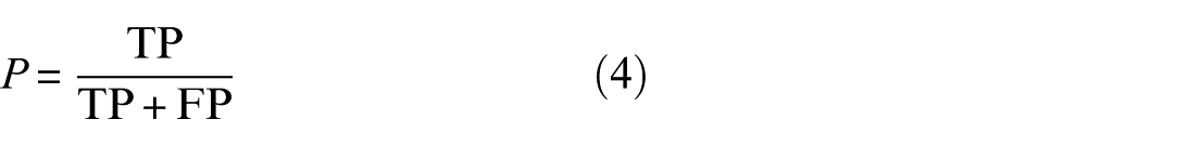
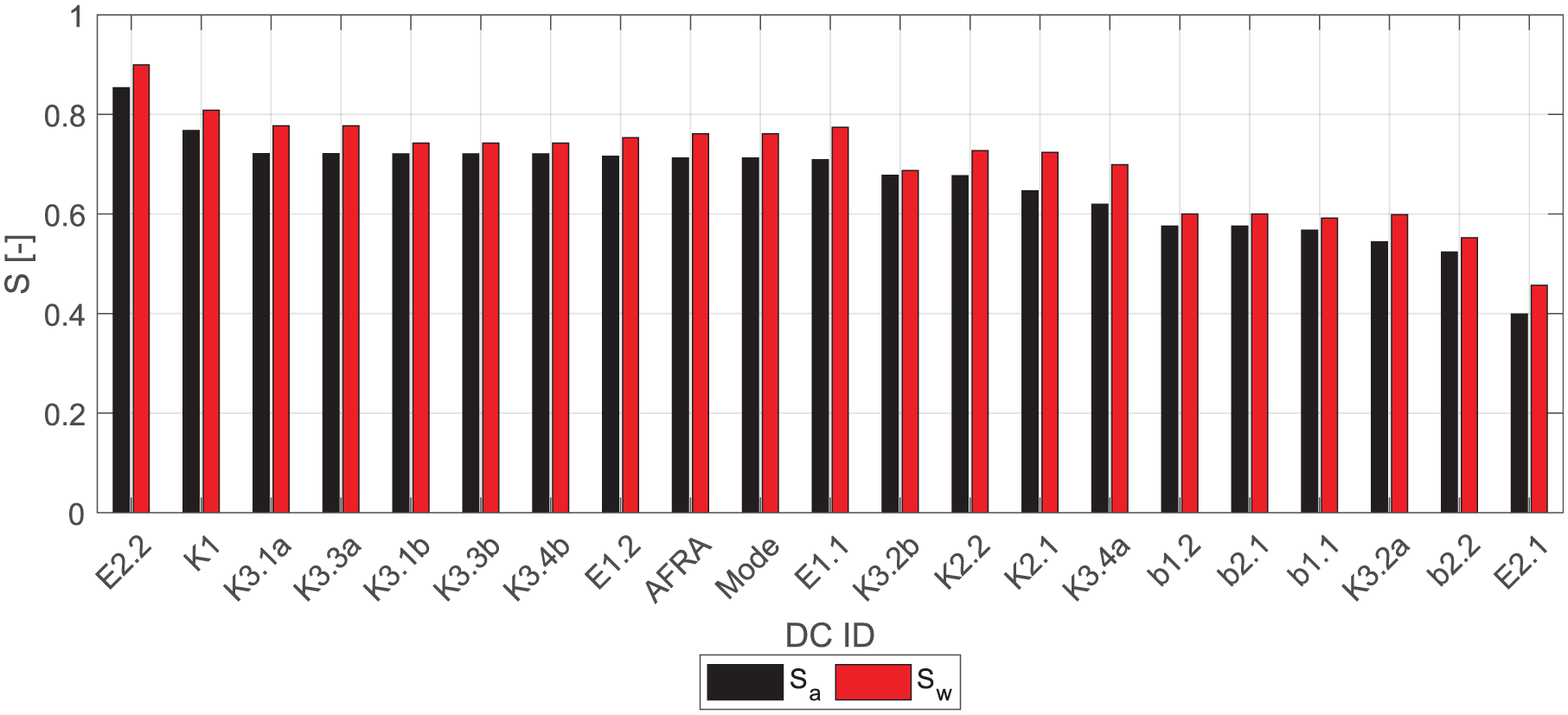
The performance evaluation of BPs was implemented according to consolidated metrics based on the confusion matrix, accounting for true positive (TP), false positive (FP), false negative (FN), and true negative (TN) conditions.^34–36 Similar method were used in the literature applications for performance evaluation in the context of AE testing.^37,38 In particular, precision (P) (Equation (4), recall (R) (Equation (5), and F1-score (F1S) (harmonic mean of P and R, Equation (6)), and accuracy (A; Equation (7)) were assessed for each DC and grouping all three DS; for this latter computation, both DC-averaged and DC-weighted computations were implemented, and weight coefficients were set equal to 1/7, 2/7, and 4/7 for ND, LD, and SD, respectively, in order to double the weight from ND to LD and from LD to SD.

P = \frac{TP}{TP + FP}

(4)

R = \frac{TP}{TP + FN}

(5)

F 1 S = 2 \frac{P R}{P + R}

(6)

A = \frac{TP + TN}{TP + TN + FP + FN}

(7)

Finally, a global score parameter (S) was defined (Equation (8)) by a weighted combination of A and F1S, setting α equal to one-third, aiming at giving double weight to F1S.

S = α A + (1 - α) F 1 S

(8)

Results and discussion

The confusion matrices are not reported for the sake of brevity, and Figure 9 shows P, R, F1S, and A associated with DSs for all DC. It should be noted that the experimental dataset was not balanced in terms of ND, LD, and SD conditions, and this might have conditioned the results, in particular, ND and LD were both associated with one-fourth cases, whereas a double number of cases was related to SD.

Figure 9.

Precision (P), recall (R), F1 score (F1S), and accuracy (A) associated with DSs for all method DC.

The prediction performances in terms of all parameters depicted in Figure 9 generally have higher precision, recall, combined score (F1S), and accuracy for correctly identifying ND, whereas an opposite trend, that is, a lower prediction performance, is overall associated with LD, which corresponds to the most challengingly predictable DS over the investigated range of methods. SD predictions have performance metrics that are intermediate, but significantly better than LD ones. The fact that ND and LD had the same experimental occurrences suggests that the difference in terms of performance metrics is more likely to be associated with the more mechanically challenging identification of LD, as it was also discussed in the previous sections. The performance metrics associated with SD show that the related prediction (1) is more challenging than ND one (experimental SD occurrences are double than ND but ND precision is larger than SD one) and (2) is comparable with LD one, even though a rigorous comparison should be based on cases having the same experimental number of occurrences. As a consequence, identifying LD is a significant challenge, as evidenced by its lower performance in all metrics; accordingly, this could indicate overlap or confusion between LD and other DSs. SD is easier to classify than LD but not as consistently as ND. The results suggest a need for further refinement in identifying low-damage scenarios, as they seem to be misclassified the most often.

The more challenging detection of LD is also due to the mechanical classification. As a matter of fact, the mechanical identification of LD is inherently characterized by subtle and localized damage phenomena that affect the beam local flexural behavior without causing clear changes in its global response. While SD is univocally defined in quantitative terms, mechanical achievement of LD is more affected by uncertainty. Moreover, over the experimental tests, LD was achieved a relatively reduced number of times. This partial or limited expression of damage impacts AE generation and assessment, since the associated acoustic signatures are typically less pronounced and more prone to be masked by noise or disturbance. Finally, it should be noted that, in some cases, for example, for several K criteria and AFRA, mechanical LD was conservatively detected as SD, and this is due to both (1) the narrow mechanical transition between LD and SD and (2) the not optimized/calibrated nature of the AE criteria thresholds.

Despite the relatively challenging predictions related to LD and SD, it should be noted that, overall, the prediction performance can be considered as satisfactory, as it is quantitatively discussed in the following paragraph. Moreover, some methods and DC are highly satisfactory. The generally positive performance of the investigated set of methods/DC can be demonstrated by considering (1) the relatively high-performance metrics of the mode results (M-matrix in Figure 6) plotted in Figure 10 (i.e., see F1S associated with mode) and (2) the relatively low deviations and entropies associated with the mode (Figure 6), as previously discussed. In other words, the investigated methods likely provide a comprehensive prediction (high performance metrics associated with M-matrix) that is also potentially associated with a relatively low dispersion (low deviations in DF-matrix and reduced entropy in E-matrix). Even though the set of investigated methods, or better DC, affects the abovementioned estimations with regard to both mode and dispersion data, the abovementioned outcomes can be considered as reasonable and representative since a variety of methods and a discretely large number of DC is considered.

Figure 10.

Precision (P), recall (R), F1 score (F1S), and accuracy (A) grouped for all DSs considering average and weighted value (X_a and X_w) for all DC.

In order to comprehensively account for DSs, Figure 10 depicts P, R, F1S, and A computed synthesizing all DS data by means of average and weighted values (X_a and X_w, respectively). The unitary value represents the maximum possible performance, and this confirms previous comments regarding the overall satisfactory predictions: Mode F1S and A values range between 0.65 and 0.80, respectively. Furthermore, the most performing DC, that is, E2.2, yields F1S and A values larger than 0.90–0.95, which are highly satisfactory. In particular, the E2.2 performance metric loss from unitary values is only due to two experimental LD conditions that were classified as ND according to E2.2. The conventional definition of LD and SD as relatively LD conditions (i.e., micro and macrocracking initiation and formation) strengthens the significance of the BPs, among the overall predictions and with particular regard to the most performing DC.

Figure 10 also shows that weighing DS does not majorly affect the results in most cases, as compared to the average data, even though (a) weight coefficients were substantially unbalanced (1/7, 2/7, and 4/7 for ND, LD, and SD, respectively) and (b) they implemented the lowest weight coefficient to the least challengingly predictable DS. Specifically, maximum (average) discrepancy absolute value associated with P, R, F1S, and A corresponds to 0.153, 0.167, 0.122, and 0.167 (0.059, 0.067, 0.062, and 0.067), respectively.

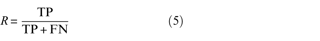
The applicative classification of the performance of the different methods and DC is based on the assessment of the global score (S), depicted in Figure 11. As it was previously discussed, E2.2 DC provides the most performing prediction, yielding S value equal to 0.85 and 0.89 for average and weighted computation (S_a and S_w), respectively. The second most performing prediction associated with K1 DC has a score approximately 10% lower than E2.2 score. Weighted computation yields higher S values, and for moderate-to-high performance estimations, the discrepancy is overall not larger than 5%, confirming the relative stability of the assessment in terms of weighting coefficients.

Figure 11.

Global score (S) grouped for all DSs considering average and weighted value (S_a and S_w) for investigated DC, considering S1 to S4 specimens and 16 tests.

A large number of DC are associated with S values just larger than 0.7, with weighted S larger than average one, having a discrepancy that increases as S decreases. This suggests that these methods might perform well but would be influenced by the DS distribution in the weighted computation. This set of DC includes some K3 DC, E1.2, AFRA, and mode estimations. The least performing DC is associated with E2.1, which significantly underperforms the penultimate DC, that is, associated with b1.1 and b2.2 estimations. Considering the different methods, b value methods provide the worst predictions, with all four DC having relatively low performance metrics (e.g., lower than mode estimation).

Overall, Kaiser method provides good predictions that are not necessarily significantly conditioned by the specific MS, and this suggests that the strong physical interpretation of Kaiser effect and Felicity ratios balances the uncertainty associated with the conventional definition of the significant activity criterion (that generates the multiple DC). Furthermore, the study showed that only specific formulations are likely to be associated with low performance (i.e., K3.2a). On the other hand, E2.2 provides the best prediction, and this confirms that entropy-based measures, in particular, cumulative Kullback–Leibler entropy with regard to the specific EC, have a high potential. In future studies, the blindly assessed E2.2 criterion should be experimentally calibrated for enhancement purposes. It is also interesting to notice that DC associated with E2.2 are compatible with DC found to be effective in past studies that focused on various metallic materials,^39–42 and this indicates that the entropy metrics and DC based on historical, especially Kullback–Leibler formulation, do not potentially depend on material/geometry and application.

Validation considering additional specimens

The developed MSs and criteria were defined blindly, and both E2.2 and K1 were found to be reliable for the detection of the flexural cracking process, from the microcracking formation (incipient deviation from linear behavior, conventionally associated with LD) to macrocracking initiation and propagation (significant and steady stiffness reduction, defined as SD). All investigated criteria, including the abovementioned ones, were assessed with regard to two additional girder specimens (namely, S5 and S6), derived from the benchmark beams. S5 and S6 were tested under the same testing protocols and loading conditions already used for S1 to S4, and further details are omitted for the sake of brevity and generality. The prestress level of S5 and S6 was the same as S1 and S2, respectively, without any external posttensioning. The instrument arrangement is depicted in Figure 12, where is can be noted that channels (Ch) 1 and 4 (2 and 3) correspond to sensor VS75 (VS150), and that Ch1, Ch2, and Ch3 are in the middle point area of the beam, with Ch3 is attached to the inferior surface of the girder and Ch1 and Ch2 are symmetrically attached to the upper part of the lateral surface of the girder. A band-pass 50–200 kHz filter was used for MS75, and for all other sensor/acquisition features, the same parameters reported in section “Acoustic emission tests” were set.

Figure 12.

Type and location arrangement of sensors associated with tests on S5 and S6 specimens (dimensions in mm).

VS75 sensors were also used to test the additional girders in order to account for the variation of the sensors, with regard to tests performed on S1–S4 specimens, which implemented sensors with lower and higher working/resonant frequencies (VS30 and VS150).

It should be noted S5/S6 Ch1 and Ch2 are located in the same position of S3/S4 Ch1 and Ch2, as well as S5/S6 Ch3 positions correspond to S4 Ch3 one, but only S3/S4 Ch2 and S4 Ch3 correspond to identical S5/S6 Ch2 and Ch3 sensors, respectively, related to VS150.

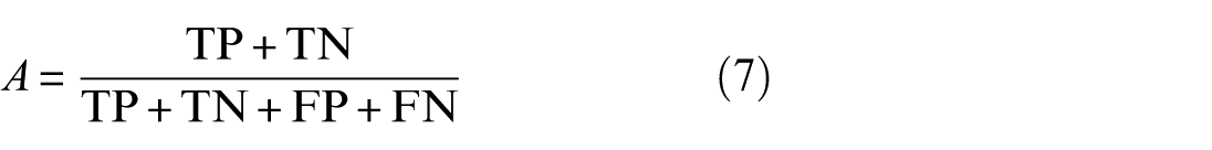
Figure 13(a) shows the F_e versus Δ curves associated with S5 and S6 specimens, where both mechanical LD and SD states and E2.2 EC attainment are depicted. SD achievement is clearly detectable on the curves as it is associated with a significant and relatively rapid stiffness reduction, whereas LD is less straightforward to identify, as was previously discussed. In particular, S5 and S6 were found to be affected by LD under P1L1 and P1L2, respectively, whereas ND was identified for earlier loading conditions. SD was detected corresponding to P1L2 and P1L3, respectively. S5 and S6 achievements are almost identical to the ones related to S1 and S2, which presented the same prestress level, and the only difference is associated with P1L1 achievement related to S1, which was more severe (SD) than the one detected for S5 (LD). It should be noted that SD achievement was achieved just below (above) F_e,1 for S1 (S2), as can be observed in Figure 6 (Figure 12), and therefore a slight variation in achievement force results in DS difference outcome.

Figure 13.

Applied force (F_e) versus deflection (Δ) curves related to S5 and S6, achievement of mechanical LD and SD states, and related EC attainment based on cumulative Kullback-Leibler entropy (E2.2 MS). EC2 and EC3 correspond to LD and SD, respectively. Ch 1, 2, and 3 correspond to VS75, VS150, and VS150 sensors, respectively.

The time evolution of the ΣH_KL curve is depicted in Figure 14 for some representative cases related to S5 and S6, together with time evolution of F_e, pointing out the EC2 and EC3 detection and the mechanical damage conditions related to LD and SD, respectively, discussed below. The differences in detection between Ch1 and Ch2 can be attributed primarily to the sensor characteristics, assuming symmetrical behavior of the beam. Sensor VS75 (Ch1) consistently detects both EC2 and EC3 earlier than VS150 (Ch2), indicating a higher sensitivity in terms of entropy measures (E2.2). A similar trend was observed for S2 when comparing the responses of the VS30 and VS150 sensors. Specifically, VS75 detects EC2 condition prior to the LD achievement, with the margin decreasing from EC2 to EC3, corresponding to the transition from LD to SD. VS150 sensors (Ch2 and Ch3) detect EC2 and EC3 closer to the occurrence of LD for S5, while the detection is less precise for S6, due to an early (or delayed) detection of LD (SD). Overall, in all cases, there is a satisfactory identification of both low and SD conditions, and the findings highlight that E2.2 entropy trend remains consistent and effective across the various setups despite the differences in sensor characteristics. As a matter of fact, similar results were found considering VS30 sensors, as previously mentioned. This confirms that the entropy-based approach, with regard to the developed criteria, provides a reliable method for damage detection, regardless of the sensor type and other variables, such as the level of prestress and the retrofitting interventions.

Figure 14.

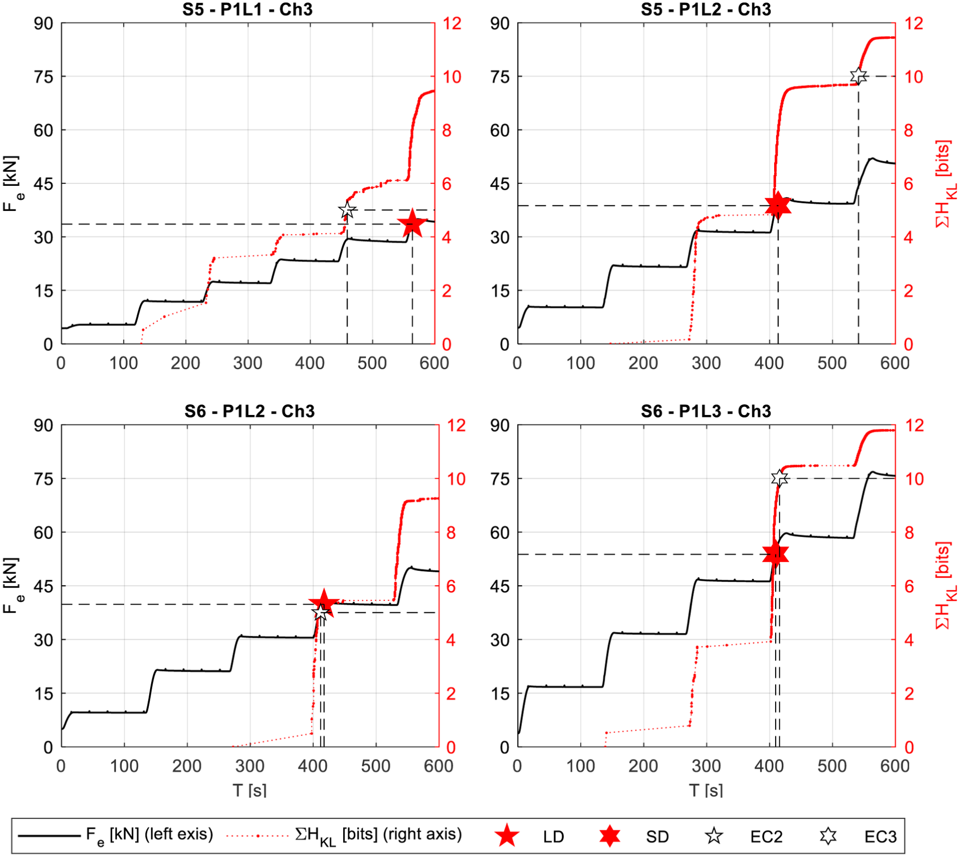
Applied force (F_e) versus time (T) curves (left axis) and cumulative Kullback–Leibler entropy (E2.2 MS) (ΣH_KL) versus time (T) associated with achievement of mechanical LD and SD) states, corresponding to P1L1 (P1L2) and P1L2 (P1L3) for S5 and S6, respectively. The curves are related to Ch3, corresponding to VS150 sensor.

K1 MS detected SD corresponding to P1L1 and P1L2, respectively, and ND was detected for preceding protocol. Similar trends similar to the S1 to S4 results were found considering the other MSs.

K1 almost provides the same estimations associated with E2.2, and the only difference is related to a more accurate but less conservative E2.2 identification of LD for S2 under P1L2. The slightly more conservative estimation of K1 aligns with proof-test objectives of the MS.

Experimental calibration and final corroboration

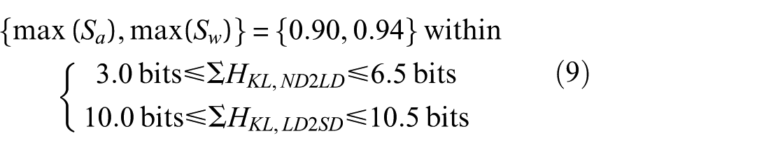
E2.2 was found to be the best MS over BPs, and, in this section, E2.2 EC (ΣH_KL) thresholds are experimentally calibrated considering the complete set of six specimens. In particular, S is computed are computed over the variation of both EC thresholds, that is, (1) ND to LD ΣH_KL limit, ΣH_KL,ND2LD, and (2) LD to SD ΣH_KL limit, ΣH_KL,LD2SD, blindly set equal to 5 and 10 bits, respectively; the former (latter) is varied from 2 to 8 (8–13) bits in the parametric analysis. The resulting S versus {ΣH_KL,ND2LD,ΣH_KL,LD2SD} surface is depicted in Figure 15. For both average and weighted S computations, maximum S is defined in the range reported in Equation (9) for average S (S_a) and weighted S (S_w).

\begin{matrix} {max (S_{a}), \max (S_{w})} = {0.90, 0.94} within \\ {\begin{matrix} 3.0 bits \leq Σ H_{KL, ND 2 LD} \leq 6.5 bits \\ 10.0 bits \leq Σ H_{KL, LD 2 SD} \leq 10.5 bits \end{matrix} \end{matrix}

(9)

Figure 15.

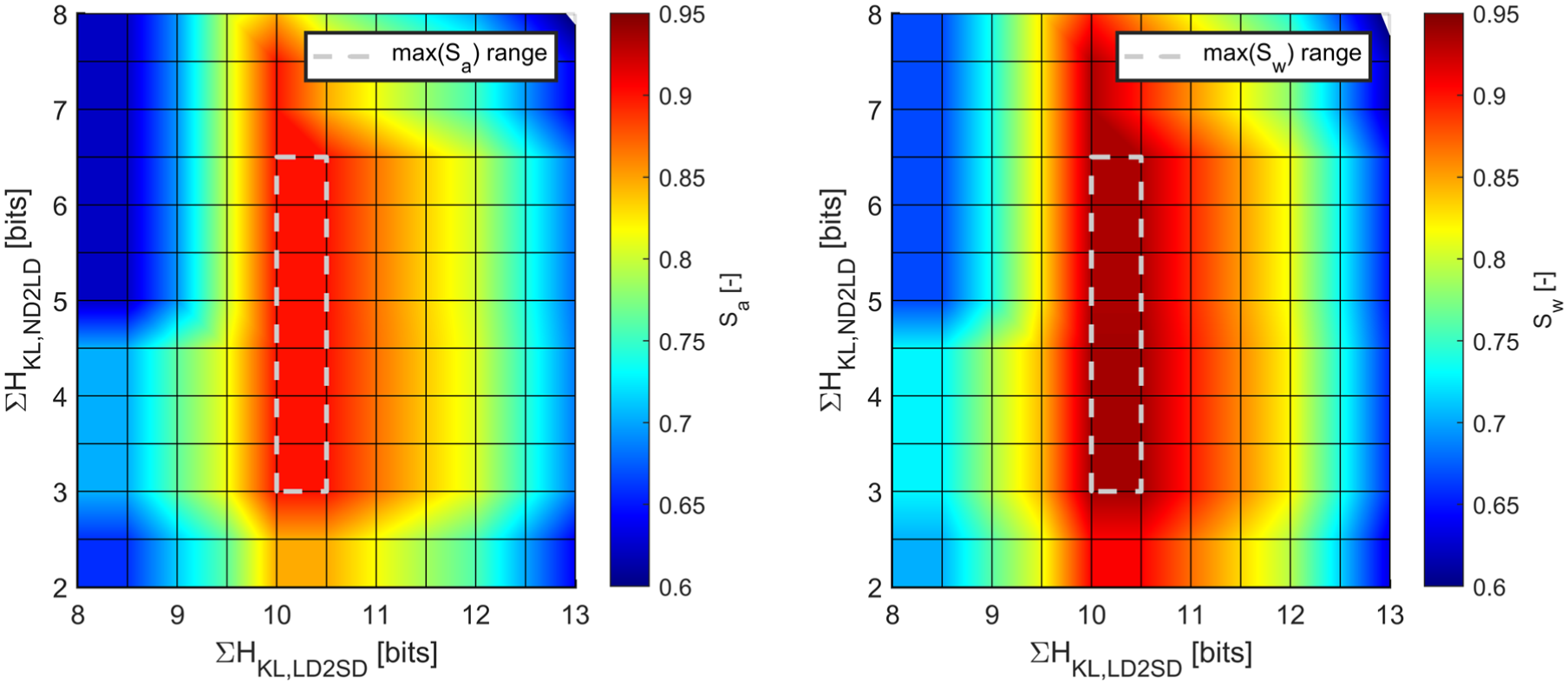
Average and weighted global scores (S_a and S_w) as a function of EC thresholds associated with cumulative Kullback–Leibler entropy ΣH_KL (E2.2), that is, ΣH_KL,ND2LD and ΣH_KL,LD2SD, considering S1 to S6 specimens and 24 tests.

It is interesting to note that optimum ΣH_KL,ND2LD range is associated with a relatively large range of entropy, showing that exceedance of a relatively low threshold, for example, 3.0 bits, is a sufficient condition for a major increase up to relatively large values and a necessary and sufficient condition for LD achievement, and this strengthens the robustness of the criterion. In other words, once the threshold is exceeded, the damage classification is not sensitive to the amount of the entropy increase.

Damage classification and assessment effectiveness is highly sensitive to ΣH_KL,LD2SD and the optimum entropy range is narrow. The first tentative EC threshold values determined in the context of BPs are included within the optimum range, but more conservative optimum EC criteria can be assumed as reported in Equations (10)–(12), recalling that these were calibrated considering six specimens under four loading protocol each, resulting in 24 tests.

{EC}_{1} : Σ H_{KL} < 3.0 bits

(10)

{EC}_{2} : 3 bits \leq Σ H_{KL} < 10.0 bits

(11)

{EC}_{3} : Σ H_{KL} \geq 10.0 bits

(12)

As a final corroboration, S was recomputed for all MSs using the complete dataset of six specimens. The results, presented in Figure 16 (specimens S1–S6) in terms of both average and weighted S values, show good consistency with those from Figure 11 (specimens S1–S4). In particular, the inclusion of the two additional specimens (S5 and S6) does not significantly alter the S scores. Overall, S tends to remain stable or to increase slightly when moving from four to six specimens (from 16 to 24 tests). Notably, E1.1, AFRA, and E1.2 estimations, already associated with similar satisfactory S values for specimens S1 to S4 (Figure 11), exhibit an upward trend and, following the E2.2 criterion, emerge as the most effective ones. K1 criterion remains satisfactory but yields a slightly lower S score than these top-performing MSs.

Figure 16.

Global score (S) grouped for all DSs considering average and weighted value (S_a and S_w) for investigated DC, considering S1 to S6 specimens.

The final assessment, based on 6 specimens and 24 tests, confirms and reinforces the validity of the proposed criteria, supporting their potential application in the development of SHM procedures.

Conclusions

Summary

The article develops and evaluates damage assessment criteria based on AE testing for the identification of low and moderate cracking damage conditions in prestressed RC girders. Six specimens were tested under four-point bending tests according to cyclic and monotonic procedures. AE data were detected, and multiple analysis methods and MSs were tested through a blind evaluation of DSs associated with each test. The effectiveness of the proposed criteria was quantitatively assessed against the experimental results, by means of a score (S) ranging from zero to one, leading to their validation and, for the best-performing MS, to a dedicated calibration effort.

Key results and discussion remarks

Key results and discussion remarks are summarized in the following.

Genuine AEs sourced by crack onset and propagation could be potentially detected by more than 1–1.5 m distances, even though with reduced entity, under the tested conditions and used equipment. The use of sensors resonant in the 75–150 kHz range is preferable, and acquisition parameters can be optimized following the indications of this study. It is recommended to deploy four sensors for each expected damage zone.

Kaiser effect and Felicity ratio analysis confirmed a solid alignment with mechanical response, especially with regard to K1 MS, which yielded an S value equal to about 0.75. The method overall was effective in identifying damage onset and accumulation through controlled loading tests. The study proposes potentially effective specifications for the conventional identification of significant AE thresholds.

AFRA analysis revealed that an increase in RA and decrease in AF reflects the evolution of damage, expanding the traditional scope of AFRA, which is typically focused on crack type identification. In particular, AFRA was associated with an S value equal to about 0.8. Furthermore, it should be noted that AFRA-based criterion relies on trend analysis rather than absolute values or specific criteria, and this strengthens its potential robustness for application under significant uncertainties (e.g., in situ monitoring).

b-value might be correlated with damage evolution but with less clarity and robustness of other investigated methods. The effectiveness of this latter method was found to be conditioned by the specific case and applications. Its performance appeared more case- and noise-dependent, and overall, it was deemed less effective, for example, the highest S over the investigated b-value MSs was equal to about 0.6. This underperformance may derive from the fact that b-value analysis primarily relies on amplitude and amplitude-based event frequency correlations, which are inherently more susceptible to noise. In contrast, other methods, such as entropy-based ones, are less affected by noise and disturbance as they indirectly incorporate filtering/cleansing mechanisms. In summary, b-value analysis could yield better results when effective noise-filtering procedures are implemented or when the signal environment is relatively clean, unlike other techniques that are intrinsically more robust to such disturbances.

AE entropy analysis was found to be potentially well correlated with damage initiation and evolution, showing a clear pattern related to the absolute and cumulative computations, especially with regard to E2.2 MS. Entropy parameters were reasonably stable, and their trends did not depend on the specific test, also highlighting a relatively low sensitivity in terms of value ranges to different testing arrangements and sensors. In particular, E2.2 yielded an S value equal to about 0.9, whereas the other ones, except E2.1, resulted in larger than 0.8. E2.1 provided an S value equal to about 0.4. Only E2.2 criterion was calibrated within this study, and the performance of the other (entropy-based) MSs could further improve with optimized calibration. Additionally, since the entropy criteria were implemented using a threshold-based approach, alternative methods, such as those based on gradient and gradient variation,³⁹ may provide better results, particularly for E2.1 that does not work well with thresholds.

The validation highlighted the role of sensor characteristics, with higher sensitivity to E2.2 as the sensor resonant frequencies decrease. Despite these variations, the entropy-based E2.2 criterion consistently identifies DSs across different setups, proving its robustness.

The significance of the developed MSs is strengthened by recalling that the focus was on minor damage conditions: (1) LD condition is not generally visible since the related cracks have relatively reduced widths (e.g., lower than 0.1 mm) and extension and (2) SD condition does not represent an actual structural damage condition, but represents the effective initiation of the postcracked response.

Implementation in structural health monitoring (SHM)

The following remarks support the implementation of the investigated MSs for SHM purposes.

The sensor characteristics, among the tested frequency ranges (i.e., from 30 to 150 kHz resonant sensors) and related filtering (Sections “Acoustic emission tests” and “Validation considering additional specimens”), influence the AE sensitivity to damage and noise, which decreases as resonant frequency increases. However, the comparisons among the different specimens demonstrate that the assessment based on most effective MSs is not affected by the variation of the sensors, and 75–150 kHz resonant sensors are recommended as they balance AE sensitivity to noise and clear detection of genuine events.

The AE acquisition parameters adopted in the study are explicitly reported, and additional implementation guidance can be provided by the corresponding author upon reasonable request.

The criteria were validated using commercial wideband AE sensors and standard acquisition systems, requiring only moderate sampling rates and a minimum of four sensors per damage-prone area, which can be adjusted based on monitoring needs.

Entropy-based and AFRA criteria appear well suited for passive monitoring of RC girders subjected to (a) increasing load or deformation conditions (e.g., as a stop criterion during proof-testing^43,44), and potentially (b) bridge service conditions. K1 criterion could be suitable in the context of proof-testing and load–unload testing protocols, where the applied load is explicitly known and controlled.

The proposed DC are computationally lightweight and based on simple statistical operations, making them suitable for real-time and time-continuous SHM applications. Several MSs (e.g., E2.2 and AFRA) have been successfully tested on commercial AE software supporting real-time evaluation, and their simplicity allows for future implementation on embedded or low-power computing platforms.

Limitations and potential developments of the study

The effectiveness of the developed criteria refers to the tests performed but might be extended to other similar or comparable cases, with due consideration. While the findings confirm the potential of the proposed methods for damage classification, the limited number of specimens (six girders under four loading protocol each, resulting in 24 tests) and associated statistical constraints must be acknowledged, especially regarding the potential implementation in situ.

The more challenging detection of LD is also attributable to the uncertainty of its mechanical classification, which is based on subtle, localized damage affecting only the beam local flexural behavior without altering the global response. Moreover, limited (LD) occurrence in the experimental tests and low-intensity AE signatures it generates made LD more difficult to identify. This often led to conservative misclassification as SD, especially when AE thresholds were not specifically calibrated. Therefore, further tests should focus more on damage initiation phenomena, addressing the issue from a microscopical point of view and also considering the material scale.

Finally, future work will focus on refining the processing logic for each MS, exploring more suitable calibration approaches, and integrating additional physical data to enhance the validation of prediction outcomes. A larger and more diverse experimental dataset, including tests in situ, will be considered to strengthen the statistical significance and general applicability for SHM purposes.

Footnotes

Acknowledgements

The contribution of Eng. Giuseppe Pollio and Eng. Dario Chiacchia for operative testing support and data management are appreciated. E.T.S. Sistemi Industriali Srl (Eng. Alberto Monici) (https://www.etssistemi.com/) and Vallen Systeme GmbH (/) are thanked for the technical and operative support.

Declaration of conflicting interests

The authors declared no potential conflicts of interest with respect to the research, authorship, and/or publication of this article.

Funding

The authors disclosed receipt of the following financial support for the research, authorship, and/or publication of this article: The study was supported by the following projects: (a) ROCK-RESILIENCE: ROCKing-based strategies for RESILIENCE of reinforced concrete structures: conception, structural design, nonstructural components, efficiency and sustainability – CUP: E53D2301704001 (European Union Next-Generation EU – Piano Nazionale di Ripresa e Resilienza (PNRR) – MISSIONE 4 COMPONENTE 2, INVESTIMENTO N. 1.1, BANDO PRIN 2022 PNRR D.D. 1409 del 14-09-2022), (b) Progetto di sviluppo del Dipartimento di Strutture per l’Ingegneria e l’Architettura “Dipartimento di Eccellenza” 2023-2027 (Italian Ministry of University and Research, MUR), (c) Progetto di rilevante interesse nazionale (PRIN) 2020YKY7W4 “ENRICH: ENhancing the Resilience of Italian healthCare and Hospital facilities” (Italian Ministry of University and Research, MUR), (d) Progetto di rilevante di interesse nazionale (PRIN) 2020P5572N “FIRMITAS: multi-hazard assessment, control and retroFIt of bridges for enhanced Robustness using sMart IndusTriAlized Solutions” (Italian Ministry of University and Research, MUR), and (e) Progetto “RESIST RobustnEss aSsessment and retrofItting of bridgeS to prevenT progressive collapse under multiple hazards” (University of Naples Federico II and Compagnia di San Paolo through STAR Plus Programme 2020).

Ethical considerations

There are no human participants in this article and informed consent is not required.

ORCID iDs

Danilo D’Angela

Gennaro Magliulo

Daniele Losanno

Fulvio Parisi

Data availability

The data that support the findings of this study are available from the corresponding author, (D.D.), upon reasonable request.

References

Losanno

Galano

Parisi

Influence of strand rupture on flexural behavior of reduced-scale prestressed concrete bridge girders with different prestressing levels. Eng Struct 2024; 301: 117358.

Kang

Z-Z

Wang

, et al. A dual-sensor AE localization method for damaged steel tendon in prestressed concrete girders using waveguide rods. Struct Health Monit 2025; 0(0): 14759217251336481.

Bazzucchi

Restuccia

Ferro

Considerations over the Italian road bridge infrastructure safety after the Polcevera viaduct collapse: past errors and future perspectives. Frat Ed Integrità Strutt 2018; 12: 400–421.

Colajanni

Recupero

Ricciardi

, et al. Failure by corrosion in PC bridges: a case history of a viaduct in Italy. Int J Struct Integr 2016; 7: 181–193.

Bornn

Farrar

Park

Damage detection in initially nonlinear systems. Int J Eng Sci 2010; 48: 909–920.

Grosse

Ohtsu

Aggelis

, et al. (eds.) Acoustic emission testing: basics for research—applications in engineering. Cham: Springer International Publishing, 2022.

Abdelrahman

ElBatanouny

Dixon

, et al. Remote monitoring and evaluation of damage at a decommissioned nuclear facility using acoustic emission. Appl Sci 2018; 8: 1663.

, et al. Self-adaptive real-time clustering analysis and damage pattern recognition for steel tube confined reinforced concrete structures through acoustic emission signals. Struct Control Health Monit 2022; 29(11): e3071.

Elbatanouny

Henderson

, et al. An automated load determination approach for concrete girder bridges through acoustic emission. Adv Struct Eng 2024; 28: 13694332241289163.

10.

Bull

Rogers

Wickramarachchi

, et al. Probabilistic active learning: an online framework for structural health monitoring. Mech Syst Signal Process 2019; 134: 106294.

11.

Dexing

Enyuan

Xiangguo

, et al. Damage precursor of construction rocks under uniaxial cyclic loading tests analyzed by acoustic emission. Constr Build Mater 2019; 206: 169–178.

12.

Ercolino

Farhidzadeh

Salamone

, et al. Detection of onset of failure in prestressed strands by cluster analysis of acoustic emissions. Struct Monit Maint 2015; 2: 339–355.

13.

Shetty

Livitsanos

Van Roy

, et al. Quantification of progressive structural integrity loss in masonry with Acoustic Emission-based damage classification. Constr Build Mater 2019; 194: 192–204.

14.

Zitto

Piotrkowski

Gallego

, et al. Damage assessed by wavelet scale bands and b-value in dynamical tests of a reinforced concrete slab monitored with acoustic emission. Mech Syst Signal Process 2015; 60–61: 75–89.

15.

Castellanos-Toro

Panesso

Marulanda

, et al. Evaluation of experimental techniques for performance estimation of post-tensioned concrete beams. Constr Build Mater 2023; 393: 132131.

16.

Abdelrahman

ElBatanouny

Ziehl

PH.

Acoustic emission based damage assessment method for prestressed concrete structures: modified index of damage. Eng Struct 2014; 60: 258–264.

17.

ElBatanouny

Ziehl

Larosche

, et al. Acoustic emission monitoring for assessment of prestressed concrete beams. Constr Build Mater 2014; 58: 46–53.

18.

Omondi

Aggelis

Sol

, et al. Improved crack monitoring in structural concrete by combined acoustic emission and digital image correlation techniques. Struct Health Monit 2016; 15: 359–378.

19.

Zeng

Hartell

Soliman

Damage evaluation of prestressed beams under cyclic loading based on acoustic emission monitoring. Constr Build Mater 2020; 255: 119235.

20.

Zhang

Zarate Garnica

Yang

, et al. Monitoring shear behavior of prestressed concrete bridge girders using acoustic emission and digital image correlation. Sensors 2020; 20: 5622.

21.

Prem

Verma

Ambily

PS.

Damage characterization of reinforced concrete beams under different failure modes using acoustic emission. Structures 2021; 30: 174–187.

22.

Elbatanouny

Henderson

, et al. Condition assessment of prestressed concrete channel bridge girders using acoustic emission and data-driven methods. Structures 2024; 67: 107008.

23.

Losanno

Galano

Parisi

, et al. Experimental investigation on nonlinear flexural behavior of post-tensioned concrete bridge girders with different grouting conditions and prestress levels. J Bridge Eng 2024; 29: 04023121.

24.

ACI Committee 437. 437.1R-07: Load tests of concrete structures: methods, magnitude, protocols, and acceptance criteria. Tech Doc, American Concrete Institute, MI.

25.

Kaiser

Untersuchungen über das Auftreten von Geräuschen beim Zugversuch. PhD Thesis, https://dds.crl.edu/crldelivery/23759 (1950).

26.

Fowler

TJ.

Acoustic emission testing of fiber reinforced plastics. In: Proceedings of ASCE fall convention and exhibit. American Society of Civil Engineers, San Francisco, CA, 1977, pp.1–16.

27.

Aggelis

DG.

Classification of cracking mode in concrete by acoustic emission parameters. Mech Res Commun 2011; 38: 153–157.

28.

Colombo

Main

Forde

MC.

Assessing damage of reinforced concrete beam using “b-value” analysis of acoustic emission signals. J Mater Civ Eng 2003; 15: 280–286.

29.

Kahirdeh

Khonsari

Acoustic entropy of the materials in the course of degradation. Entropy 2016; 18: 280.

30.

Sagar

Saha

Basu

, et al. Statistics of acoustic emission waveforms in characterizing the fracture process zone in fibre-reinforced cementitious materials under mode I fracture. Struct Health Monit 2024; 23: 2083–2101.

31.

Kullback

Leibler

RA.

On information and sufficiency. Ann Math Stat 1951; 22: 79–86.

32.

Shannon

CE.

A mathematical theory of communication. Bell Syst Tech J 1948; 27: 379–423.

33.

Soltangharaei

Anay

, et al. Implementation of information entropy, b-value, and regression analyses for temporal evaluation of acoustic emission data recorded during ASR cracking. Pract Period Struct Des Constr 2021; 26: 04020065.

34.

Hussain

Al Muhammadee Janjua

Naeem Malik

, et al. Health monitoring of CNC machining processes using machine learning and wavelet packet transform. Mech Syst Signal Process 2024; 212: 111326.

35.

Manning

Raghavan

Schütze

Introduction to information retrieval. Cambridge: Cambridge University Press, 2008.

36.

Powers

DMW

. Evaluation: from precision, recall and F-measure to ROC, informedness, markedness and correlation. Mach Learn Technol 2011; 2: 37–63.

37.

Soltangharaei

Ziehl

Evaluation of ASR in concrete using acoustic emission and deep learning. Nucl Eng Des 2021; 380: 111328.

38.

May

Alam

Nayan

, et al. Acoustic emission corrosion feature extraction and severity prediction using hybrid wavelet packet transform and linear support vector classifier. PLOS ONE 2021; 16: e0261040.

39.

D’Angela

Ercolino

Bellini

, et al. Failure criteria for real-time assessment of ductile cast irons subjected to various loading conditions. Smart Mater Struct 2021; 30: 017001.

40.

D’Angela

Ercolino

Bellini

, et al. Characterisation of the damaging micromechanisms in a pearlitic ductile cast iron and damage assessment by acoustic emission testing. Fatigue Fract Eng Mater Struct 2020; 43: 1038–1050.

41.

Hosseini

Azadi

Ghasemi-Ghalebahman

, et al. Fatigue crack initiation detection in ductile cast iron crankshaft under rotating bending fatigue test using the acoustic emission entropy method. Eng Fail Anal 2023; 144: 106981.

42.

Morteza Hosseini

Ghasemi-Ghalebahman

Azadi

, et al. Crack initiation detection in crankshaft ductile cast iron based on information entropy of acoustic emission signals under tensile loading. Eng Fail Anal 2021; 127: 105547.

43.

Christensen

Zhang

Garnica

, et al. Identification of stop criteria for large-scale laboratory slab tests using digital image correlation and acoustic emission. Infrastructures 2022; 7: 36.

44.

Zarate Garnica

Lantsoght

EOL

Yang

, et al. Shear stop criteria for reinforced concrete slab strips. In: Jensen

Frangopol

Schmidt

(eds) Bridge maintenance, safety, management, digitalization and sustainability. London: CRC Press, pp.341–349.