The use of reinforced learning to support multidisciplinary design in the AEC industry: Assessing the utilization of Markov Decision Process

Abstract

While the design practice in the architecture, engineering, and construction (AEC) industry continues to be a creative activity, approaching the design problem from a perspective of the decision-making science has remarkable potentials that manifest in the delivery of high-performing sustainable structures. These possible gains can be attributed to the myriad of decision-making tools and technologies that can be implemented to assist design efforts, such as artificial intelligence (AI) that combines computational power and data wisdom. Such combination comes to extreme importance amid the mounting pressure on the AEC industry players to deliver economic, environmentally friendly, and socially considerate structures. Despite the promising potentials, the utilization of AI, particularly reinforced learning (RL), to support multidisciplinary design endeavours in the AEC industry is still in its infancy. Thus, the present research discusses developing and applying a Markov Decision Process (MDP) model, an RL application, to assist the preliminary multidisciplinary design efforts in the AEC industry. The experimental work shows that MDP models can expedite identifying viable design alternatives within the solutions space in multidisciplinary design while maximizing the likelihood of finding the optimal design.

Keywords

Design evaluation multidisciplinary design reinforced learning Markov Decision Process social impact architecture,engineering,and construction industry

Introduction

Design development in the architecture, engineering, and construction (AEC) industry heavily depends on evaluating the merit of many alternatives against an ever-expanding list of criteria or performance metrics. AEC industry design teams’ ability to adequately evaluate possible alternatives is bound by the available resources, including time and budget. Constraining the evaluation of design due to resource limitations can lead to overlooking solutions that may be better suited for the problem. In this context, the design team’s experience can maximize resource utilization by reducing the number of viable alternatives through filtering infeasible or far-fetched design alternatives. Nevertheless, depending on the design team’s experience may result in overlooking better-performing design alternatives with which the design team has limited knowledge. Moreover, the rapid pace at which technology is changing the AEC industry renders the reliance on design teams experience less efficient and necessitates rethinking the design process.

Conventionally, the AEC industry’s design process is approached as a creative endeavour, where subjective factors, such as experience and the sense of beauty, play a significant role in the early phases of design. This approach delays the introduction of objective assessment mechanisms and limits their potential benefits. Rethinking the design problem as a decision-making problem, as Herbert Simon proposed in the 1960s,¹ allows design teams to build on the accumulated knowledge in decision-making theory to assess design alternatives objectively. Following this thinking paradigm (i.e. thinking of engineering design as a decision-making problem) entails approaching the engineering design problem as an iterative process that consists of a series of action points at which the design team is expected to make decisions.² Each decision comes with consequences, e.g. an increase in the building/manufacturing cost or a reduction in the product’s lifespan; some consequences are desirable while others are not. This process is repeated until the design team is satisfied with the aggregated consequences of all the decisions.

Many researchers have developed frameworks and tools that embrace the decision-making approach of engineering design. Examples can be seen in the several multi-criteria building systems design frameworks,^3–5 environmentally friendly concrete element design,^6,7 optimizing the environmental performance of buildings,⁸ and in the value-driven design of the aeronautics industry.^1,9–12 In these endeavours, the design deliverables’ features are linked with their potential impacts on selected performance metrics and assessed according to that impact. Indeed, the developed frameworks and tools facilitate the transition into the decision-making mentality among engineering designers. Nevertheless, the effort required to declare the links between the design deliverables’ components and the assessment criteria is far from simple and could hinder the sought transition. Artificial intelligence (AI) can aid in such processes by developing functions and algorithms that systematically link key design input parameters to identified outcome performance metrics¹³

Of the several available AI techniques, reinforced learning (RL) shows a striking resemblance to the engineering design’s decision-making approach.¹⁴ In RL, an agent progressing through a series of states (or decision points) is rewarded for making desirable decisions and penalized otherwise. The agent goes through the same process multiple times until it finds the sequence of decisions that maximizes its reward. There have been several attempts to implement RL represented in the Markov decision process (MDP) to support design efforts in several engineering disciplines, such as in ship design.^15–17 Markov decision process was also utilized to support design efforts in the AEC industry, such as the design of trusses,¹⁸ building structural frames,¹⁹ and windows.²⁰ However, RL remains underutilized in the AEC industry²¹ and with a scope limited to one discipline. Thus, the present research aspires to assess the practicality and the role of RL in supporting multidisciplinary design in the AEC industry.

In a previous endeavour,¹⁴ the authors explored the possible application of MDP to aid multidisciplinary design efforts in the AEC industry. The reported results indicated promising potentials for pairing MDP with design endeavours. The experiment, however, was primitive and lacked the required level of details to draw definite conclusions concerning the use of MDP to support design efforts. In the present research, we take the experiment further by:

• Incorporating all the components of the MDP model;

• Using real-life data to develop the MDP model of the problem; and

• Evaluating the impact of the model parameters on the identified performance outcomes.

The rest of the paper is organized as follows. The following section discusses the research methods and materials. The methods and materials section provides a brief mathematical background of the MDP model, a description of the design problem, and the design problem’s MDP model development. We then present the results of the experiment, a section that is followed by a discussion of the results, where we list the research limitations and the lessons learned from this experiment.

Methods and materials

Mathematical background- MDP model

An MDP model consists of a non-empty finite set of states (S) among which an agent moves. The channels among the states are called actions, and as in the states, there is a non-empty finite set (A) that contains all the possible actions in a model.²² In addition to S and A, an MDP model has a transitional probability function $δ : S \times A \to D (S)$ that governs the transition among states. The function δ gives the probability of selecting a state s_i+1 given a state $s_{i} \in S$ and an action $a_{i} \in A$ were chosen previously, i.e. $δ (s_{i}, a_{i}) (s_{i + 1}) = P r (s_{i + 1} | s_{i}, a_{i})$ . The definition of S, A, and δ allows us to create a new subset Dest(s,a) ⊂ S that contains all possible successors of a state s provided a.

As the agent moves between sequential states, the states it chooses form a sequence $s_{0}, s_{1}, s_{2}, \dots, s_{n}$ , which is called a play, and a policy (π) is a specific sequence of states.²³

Every time the model’s agent lands on a new state, it is either rewarded to convey the user’s satisfaction or penalized to indicate the user’s dissatisfaction with the agent’s selection. As such, for each state s and action a there is a reward (or a penalty) expressed by a reward function $r : S \times A \to ℝ$ , and the rewards are accumulated rewards as the agent progresses. It should be noted that given the MDP model’s stochastic nature, the accumulated reward at a state s of a policy π is not deterministic. Instead, we calculate the expected reward of choosing action a from a state s, provided the agent follows policy π (or Q^π(s, a)), as per equation (1).²⁴

Q^{π} (s, a) = r (s, a) + γ \sum_{s'} δ (s' | s, a) \sum_{a'} π (a^{'} | s^{'}) Q^{π} (s', a')

(1)

According to equation (1), the expected reward after choosing action a that leads to state s as part of policy π is the sum of the reward associated with a and s (or $r (s, a)$ ) with the sum of expected and discounted reward of all the states and actions that preceded a and s and belong to policy π. Discounting the reward at each step, using the discount factor γ, aims to balance maximizing the reward and length of the policy. By discounting every move’s reward, we encourage the agent to find the shortest path to optimality and prevent it from running in loops to increase the policy’s value.

Q^π(s, a) is usually referred to as the value function of policy π, and the goal of solving MDP is to find the policy with the maximum possible reward or Q^*(s, a), where²⁵:

Q^{*} (s, a) = \max_{π} Q^{π} (s, a)

(2)

The policy that leads to the maximum possible reward is the optimum policy or π* and shown in equation (3).²⁵

π^{*} = a r g \max_{π} Q^{π} (s, a)

(3)

For instance, consider the following play $s_{0}, s_{1}, s_{2}, s_{3}, s_{4}, s_{5}, s_{6}$ where each state is a function of previous states and the actions of the corresponding policy, based on equation (1), it is possible to write that the expected rewards at state 6 following action a or $Q^{π} (s_{6}, a)$ following policy π is the sum of the multiplication of the reward of each state by γ to the power of the state index as shown in equation (4).

Q^{π} (s_{6}, a) = E {r (s_{0}) + γ r (s_{1}) + γ^{2} r (s_{2}) + γ^{3} r (s_{3}) + γ^{4} r (s_{4}) + γ^{5} r (s_{5})}_{π}

(4)

When the states and actions are deterministic, the value function $(V^{π} (s))$ can be simplified to the sum of the reward at concerned state and the expected rewards of all proceeding states as shown in equation (5).²⁶

V^{π} (s) = r (s) + γ \sum_{s'} δ (s' | s, a) V^{π} (s')

(5)

In the case of |S| (note that |S| is the cardinality of set S and represent the number of elements in S) states, equation (5) is a set of |S| equations, one for each state, with |S| unknowns representing the expected reward of each state. As such, equation (5) can be presented as in equation (6).

V \leftarrow R + γ PV

(6)

Where R is the reward matrix and P is the transitional probability matrix. To find the maximum value, we begin with a guessed reward for each state and calculate an improved estimate.

Developing the MDP model for the design problem will elaborate on the formation and definition of the concepts explained in this section. Before that, we will introduce and define the design problem for which we are developing the MDP model.

The design problem

We will assess the potentials of using MDP models to support multidisciplinary engineering design endeavours in the AEC industry by finding design solutions for the case study, a multi-family condominium building, shown in Figure 1.

Figure 1.

A visualization of the case study building: (a) a 3D rendering of the building, (b) a floor plan for a typical floor.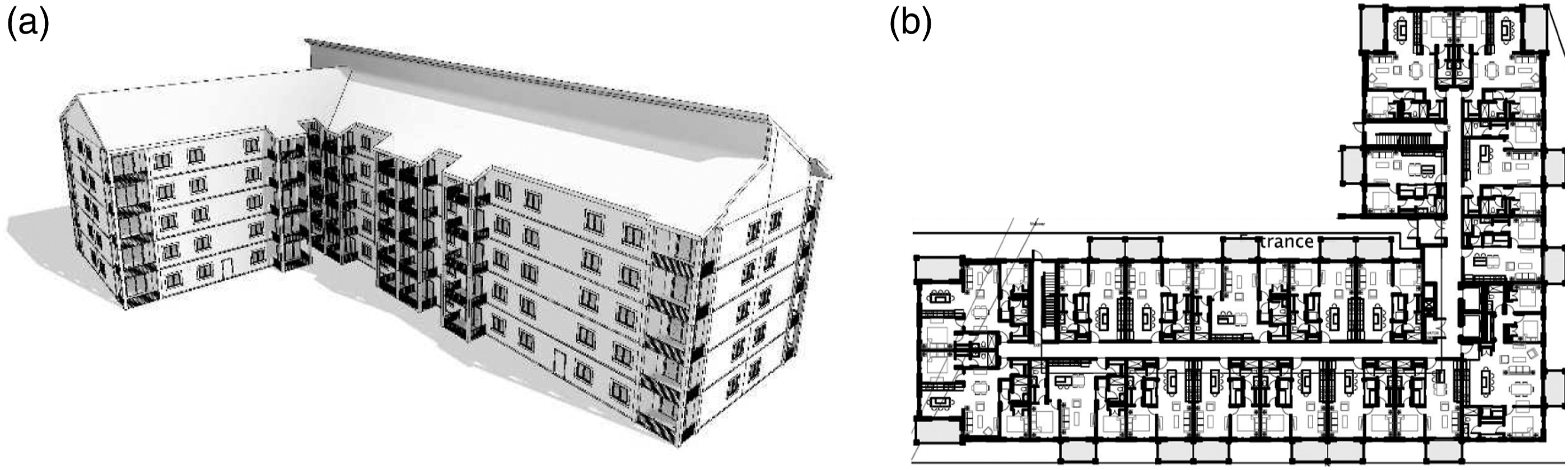

The building consists of five floors, a non-accessible attic, and an underground parkade with a total built area of 8535 m².

For the building in Figure 1, we will use an MDP model to select the best performing design alternatives for the following building systems components: heating source, heating type, construction type, roof type, flooring, exterior cladding (see Table 1). The merit of a combination of design alternatives is assessed based on the combination’s impact on the building’s construction cost, environmental impact (represented in fossil fuel consumption (FFC) measured in MJ, global warming potential (GWP) measured in CO₂-eq tonnes, and ozone depletion potential (ODP) measured in CFC-11 eq mg), and desirability.

Table 1.

The design alternatives for the building systems components of concern.

building systems component	Possible design alternatives
Heating source	natural_gas
Heating type	hot_water, forced_air, baseboard, baseboard_hot_water, heat_pump, ln_floor_heat_system, and fan_coil
Construction type	wood_frame and concrete
Roof type	asphalt_shingles, tar&gravel, epdm_membrane, and roll_roofing
Flooring	carpet__linoleum, carpet__laminate_flooring__linoleum, ceramic_tile__laminate_flooring, carpet__ceramic_tile, carpet__ceramic_tile__hardwood, laminate_flooring__linoleum, carpet__laminate_flooring, ceramic_tile__hardwood, laminate_flooring, linoleum__wall_to_wall_carpet, carpet_ceramic_tile__laminate_flooring, and carpet_ceramic_tile__linoleum
Exterior cladding	Stucco, brick__stucco, vinyl, stone__vinyl, brick__vinyl, stone__stucco, stucco__vinyl, brick, and concrete

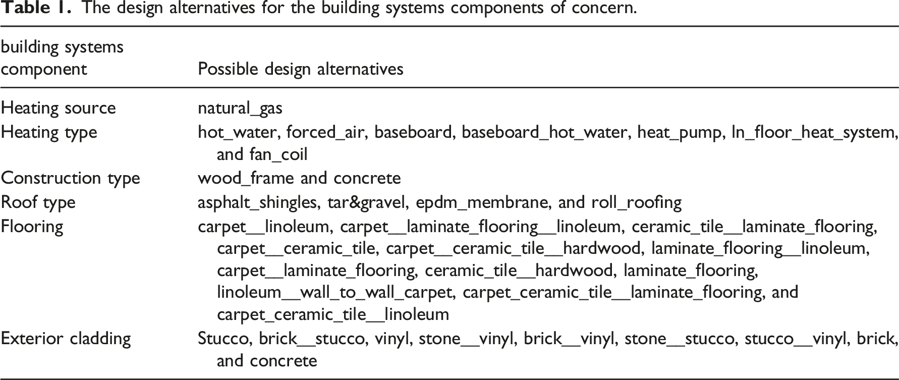
The possible design alternatives were identified by analyzing condos' features listed for sale in Edmonton, AB, Canada, between 2009 and 2019 and provided by the REALTOR® Association of Edmonton.

The combination’s impact on the mentioned performance metrics (i.e.) is evaluated considering the following assumptions:

• operational and demolishing impacts are beyond the scope of this study;

• all condos in the building have the same flooring arrangement; and,

• when an exterior cladding alternative consists of two materials, its impact is calculated considering that 75% of the building’s exterior is covered using the pair’s less impactful material. The remaining exterior is covered using the more impactful material.

RS Means® cost database and Athena environmental database are used to calculate the construction cost and the environmental impact of the design alternatives. However, it is essential to mention that due to the lack of information in the used environmental database concerning the flooring and heating system components' materials, the environmental impact during the construction phase of these components is ignored. The same applies to the heating systems’ construction cost due to the lack of cost information about heating systems assembles (there is cost data for parts but not assemblies). Finally, as a social value, the building’s desirability is measured by the predicted change imposed by a design option on the time a listed property may spend on the market when it is listed for sale, as sown in.²⁷ It should be noted that an alternative that leads to a lower time on market (TOM) for a listed property increases the building’s desirability and vice versa.

The design problem from a decision-making perspective

As the design goals and constraints are defined, it is beneficial to elaborate on the formulation of the presented design problem in the context of decision-making, before diving into the mathematical modelling realm. From the perspective of decision-making, there are six decision epochs, i.e. choosing a value for each of the following 6 features: heating source, heating type, construction type, roof type, flooring, exterior cladding. This makes a 6-dimensional solution space that contains all the possible values for each of the previously mentioned features. Nevertheless, the possible values for each feature are limited to those shown in Table 1, to balance realism and complexity in presenting the work. As a result, within the solution space, there are 6720 possible solutions, i.e. combinations of design alternatives for the features. The goal of the decision-making problem is to find the combination(s) that will concurrently minimize the construction cost, the FFC, the GWP, and the ODP, while maximizing the desirability of the building. The decision-making problem is, thus, a multi-objective optimization in a 6-dimensional space; a problem that will be explored using an MDP model.

Conventionally, design teams do not have the capacity to explore such large solution spaces due to resource limitations. Design teams, usually resort to familiar combinations widely used by developers or known to be cost effective. This, as argued before, reduces the likelihood of finding a solution that can meet several performance metrics concurrently. Consequently, not only does constructing the design problem into a decision-making allow the exploration of a large solution space, but also does allow the utilization of techniques, such as ML, that accumulate transferable knowledge and maximize the multi-aspect performance of the developed design.

It is worth mentioning that the long term objective of this work is the development of an AI-based design assistant. However, we believe that the complexity of this endeavour can only be tackled by taking small steps, which begins with using MDP in the context of optimization.

Developing the MDP model for the design problem

Given the wide use of Python in the scientific community and the availability of a Python package dedicated to solving MDP models, the development of the proposed MDP model in this research follows MDP Toolbox’s requirement for Python. By doing so, we aim to increase the present research’s reproducibility and allow the reader, using the research’s supplementary materials, to test the use of the MDP model to solve engineering design problems.

In the next sections, we will elaborate on each component of the model’s definition and development.

Define the model’s states

The design alternatives shown in Table 1 are all the possible states from which the model’s agent will choose; consequently,

S = {Natural_Gas, Hot_Water, Forced_Air, Baseboard, Baseboard_Hot_Water, Heat_Pump, ln_Floor_Heat_System, Fan_Coil, Wood_Frame, Concrete, Asphalt_Shingles, Tar&Gravel, EPDM_Membrane, Roll_Roofing, Carpet__Linoleum, Carpet__Laminate_Flooring__Linoleum, Ceramic_Tile__Laminate_Flooring, Carpet__Ceramic_Tile, Carpet__Ceramic_Tile__Hardwood, Laminate_Flooring__Linoleum, Carpet__Laminate_Flooring, Ceramic_Tile__Hardwood, Laminate_Flooring, Linoleum__Wall_to_Wall_Carpet, Carpet_Ceramic_Tile__Laminate_Flooring, Carpet_Ceramic_Tile__Linoleum, Stucco, Brick__Stucco, Vinyl, Stone__Vinyl, Brick__Vinyl, Stone__Stucco, Stucco__Vinyl, Brick, Concrete }.

Note that |S| =35.

S can be partitioned, according to the building systems components (i.e. heating source, heating type, construction type, roof type, flooring, exterior cladding), to the following subsets:

• hs = {natural_gas}

• ht = {hot_water, forced_air, baseboard, baseboard_hot_water, heat_pump, ln_floor_heat_system, fan_coil}

• ct = {wood_frame, concrete}

• rt = {asphalt_shingles, tar&gravel, epdm_membrane, roll_roofing}

• fl = {carpet_linoleum, carpet_laminate_flooring_linoleum, ceramic_tile_laminate_flooring, carpet_ceramic_tile, carpet_ceramic_tile_hardwood, laminate_flooring_linoleum, carpet_laminate_flooring, ceramic_tile_hardwood, laminate_flooring, linoleum_wall_to_wall_carpet, carpet_ceramic_tile_laminate_flooring, carpet_ceramic_tile__linoleum}

• ec = {stucco, brick_stucco, vinyl, stone_vinyl, brick_vinyl, stone_stucco, stucco_vinyl, brick, concrete}

In addition to facilitating the presentation of the next sections, these subsets assist in guiding the MDP agent’s choice at each state. This is important because the agent must select at least one design alternative for each building systems components. If the selection process is not guided (i.e. if S is not divided into subsets), the agent may opt to skip some building systems components’ design alternatives due to their low rewards compared to other alternatives. In other words, the subsets make it possible to direct the agent to choose an alternative for each building feature, as will be demonstrated in the next section.

Define the model’s actions

The present research aims to solve a design problem and build machine knowledge to be transferred for future applications. Building knowledge necessitates giving the MDP agent the freedom to roam the solution space and commit mistakes to acquire knowledge. Solving the design problem, on the other hand, requires directing the agent movement to ensure that it selects an alternative for each building system component. To balance between the agent’s freedom of choice and the requirement of the design problem, we establish the following rules for the agent’s movement:

1. the agent can hold its choice, change it to an alternative from the same subset, or choose an alternative that was chosen in a previous move; and,

2. a policy must contain at least one design alternative for each of the studied building systems components.

Following the first rule, the agent can take one of the following actions.

1. Move to a new state (denoted as F). The new state must not be previously selected or belong to the same subset as the current state. For instance, considering the agent’s starting state $s_{0} = w o o d_f r a m e \in c t$ then $D e s t (s_{0}, F) = S / c t$ . Acting F from a state s means that s is a play in the optimum policy.

2. Move to a state within the same subset (denoted as W). Acting W implies choosing an alternative for the next state that belongs to the same subset as the current state. Say that $s_{i} \in f t$ , then: $D e s t (s_{i}, W) = f t / {s_{i}}$ .

3. Move to a previously selected state (denoted as B); this action allows the agent to choose any of the states the agent has selected before its current state. Where p_selected is the set that contains all the selected states before i, then $D e s t (s_{i}, B) = p_s e l e c t e d$ . Whether the agent chooses to act W or B from a state s, it sends a message that s is not part of the optimum policy.

4. End the iteration (denoted as E). Like F, an action F from a state s indicates that s is part of the optimum policy.

Before discussing the compliance with the second rule, it is worth mentioning that there may be more than one design alternative for a given building systems component that leads to the maximum possible reward. Therefore, the second rule states to choose “at least one design alternative.” The discussion section provides further elaboration on this point. Now, to comply with the second rule, actions F and E will be restricted as follows.

1. Action F allows the agent to move in the following sequence: $h s \overset{F}{\to} h t \overset{F}{\to} c t \overset{F}{\to} r t \overset{F}{\to} f l \overset{F}{\to} e c$ .

2. Action E is allowed only when $s_{i} \in e c$ .

3. Action F is not permitted when $s_{i} \in e c$ .

Given the established action F sequence, there are two ways to approach action B; restricted and free B flows.

In the restricted flow approach, action B forces the agents to move in an inverted F sequence (i.e. $e c \overset{B}{\to} f l \overset{B}{\to} r t \overset{B}{\to} c t \overset{B}{\to} h t \overset{B}{\to} h s$ ). For instance, if the model’s agent decides to act B from $s_{i} = R o l l_{R o o f i n g} \in r t$ then $D e s t (s_{i}, B)$ is a set that contains all the states that have been selected before s_i AND belong to ct.

In the free B flow, the agent can select any previously selected state regardless of its subset. For mathematical modelling purposes, we identified five possible variations of B, based on the number of subsets the agent can jump backward. For instance, action B1 means the agent can choose from the subset that immediately precedes the subset of the current state in the B sequence (i.e.

e c \overset{B}{\to} f l \overset{B}{\to} r t \overset{B}{\to} c t \overset{B}{\to} h t \overset{B}{\to} h s

), action B2 allows the agent to skip one subset and jump directly to one before, action B3 enables the agents to jump two subsets. Table 2 shows the proposed range of actions for the free B movement.

Table 2.

The B actions and their possible moves when the agent has free B movements.

Action	Possible moves
B1	$e c \overset{B 1}{\to} f l \overset{B 1}{\to} r t \overset{B 1}{\to} c t \overset{B 1}{\to} h t \overset{B 1}{\to} h s$
B2	$r t \overset{B 2}{\leftarrow} e c$
	$c t \overset{B 2}{\leftarrow} f l$
	$h t \overset{B 2}{\leftarrow} r t$
	$h s \overset{B 2}{\leftarrow} c t$
B3	$c t \overset{B 3}{\leftarrow} e c$
	$h t \overset{B 3}{\leftarrow} f l$
	$h s \overset{B 3}{\leftarrow} r t$
B4	$h t \overset{B 4}{\leftarrow} e c$
B4	$h s \overset{B 4}{\leftarrow} f l$
B5	$h s \overset{B 5}{\leftarrow} e c$

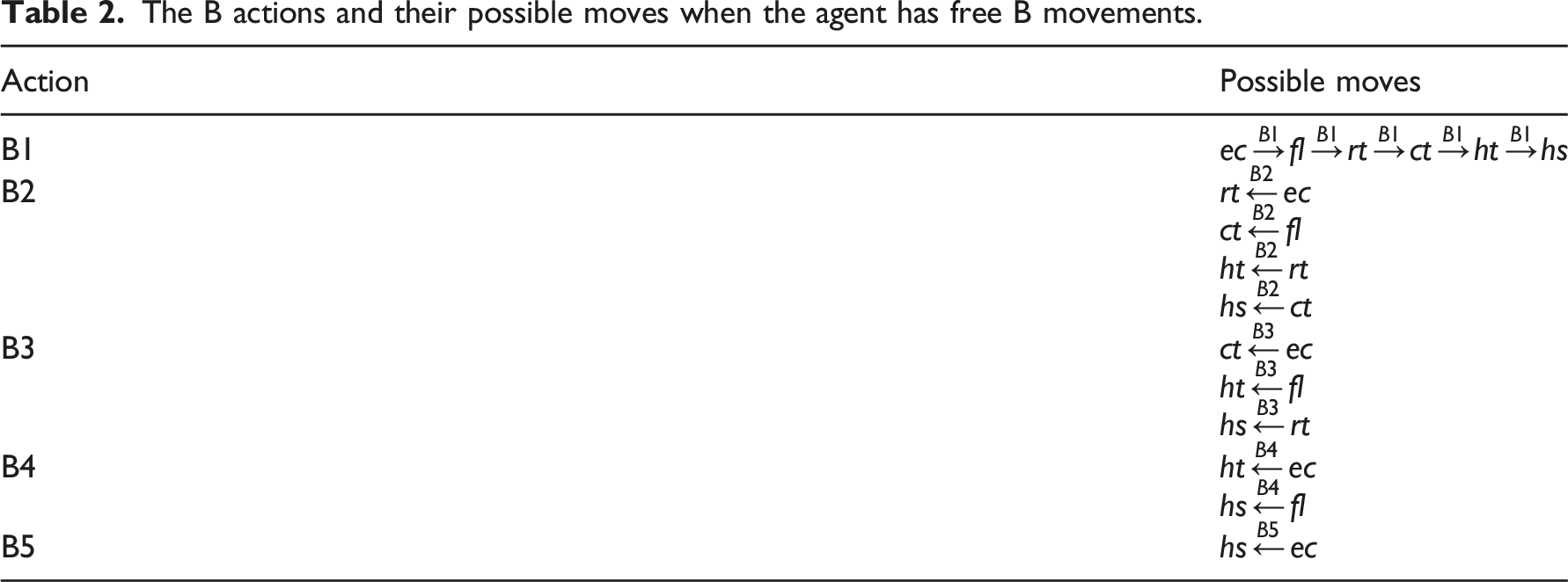
Considering the two identified approaches for B, it possible to define two MDP models; the M1 model, where the agent has restricted B movement, and the M2 model, where the agents have free B movement. Figure 2 is a graphical comparison between the two models.

Figure 2.

The possible actions between the elements of the subsets: (a) M1’s all possible actions and (b) M2’s B actions.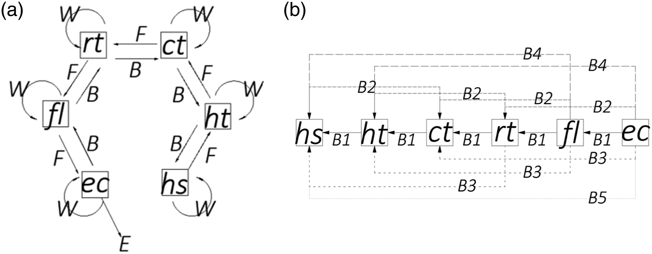

Note that actions F, W, and E of M1 and M2 are identical and, therefore, are not shown in Figure 2(b) to enhance readability.

Developing the transition probability matrix

The transition probability matrix (or P) that appears in equation (6) is an |S|×|S| matrix, where S is the set of all states with |S| =35 (as described earlier), in which $P (i, j) = P r (s_{j} | s_{i})$ . However, in MDP, s_j is dependent on both s_i and a. Consequently, we define the transitional probability matrix P (|S|×|S| matrix) for an action a as follows.

P^{a} (i, j) = δ [(s_{i}, a), (s_{j})] = P r (s_{j} | s_{i}, a)

(7)

The transitional probability matrix for the entire model (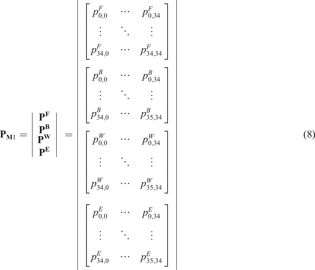P) is, then defined as an |S|×|S|×|A| (i.e. P consists of |A| matrices of |S|×|S|, where A is the set that contains all the actions in the model and |A| is the number of actions in the model). In the case of the present research, there are two models; M1 and M2. In M1, there are four actions, i.e. F, B, W, and E, and, therefore, P_M1, the transitional probability matrix for model M1, is a set of four matrices of 35 × 35 as depicted in equation (8). Likewise, model M2 has eight actions, i.e. F, B1, B2, B3, B4, B5, W, and E, so its transitional probability matrix (P_M2) is a set of eight matrices of 35 × 35 as in equation (9). In these matrices, an element $p_{i j}^{a}$ indicates the probability of choosing state j given state i and action a.

P_{M 1} = | \begin{matrix} P^{F} \\ P^{B} \\ \begin{matrix} P^{W} \\ P^{E} \end{matrix} \end{matrix} | = | \begin{matrix} [\begin{matrix} p_{0,0}^{F} & \dots & p_{0,34}^{F} \\ ⋮ & ⋱ & ⋮ \\ p_{34,0}^{F} & \dots & p_{34,34}^{F} \end{matrix}] \\ [\begin{matrix} p_{0,0}^{B} & \dots & p_{0,34}^{B} \\ ⋮ & ⋱ & ⋮ \\ p_{34,0}^{B} & \dots & p_{35,34}^{B} \end{matrix}] \\ \begin{matrix} [\begin{matrix} p_{0,0}^{W} & \dots & p_{0,34}^{W} \\ ⋮ & ⋱ & ⋮ \\ p_{34,0}^{W} & \dots & p_{35,34}^{W} \end{matrix}] \\ [\begin{matrix} p_{0,0}^{E} & \dots & p_{0,34}^{E} \\ ⋮ & ⋱ & ⋮ \\ p_{34,0}^{E} & \dots & p_{35,34}^{E} \end{matrix}] \end{matrix} \end{matrix} |

(8)

P_{M 2} = | \begin{matrix} P^{F} \\ \begin{matrix} P^{B 1} \\ P^{B 2} \\ \begin{matrix} P^{B 3} \\ \begin{matrix} P^{B 4} \\ P^{B 5} \end{matrix} \end{matrix} \end{matrix} \\ \begin{matrix} P^{W} \\ P^{E} \end{matrix} \end{matrix} |

(9)

Note that matrices P^F, P^W, and P^E are the same for P_M1 and P_M2.

Calculating the values of $p_{i j}^{a}$ follows the process in Figure 3.

Figure 3.

The process of calculating the transitional probabilities of the model.

The development of P_M1 and P_M2 in the present work depends on the statistical co-occurrence of building features. The co-occurrence of building features is studied using the association analysis on a dataset containing 63,694 condos, with their features listed for sale in Edmonton (the capital city of the Canadian province of Alberta) between 2009 and 2019. The association analysis yields the most frequent combinations of the studied features. In the current research, the association analysis led to 395 different combinations of the alternatives listed in Table 1 and their frequencies, i.e. the number records in which a given combination was observed. Based on its frequency ( $f r e q u e n c y_{c_{i}}$ , the number of times the combination is detected in dataset) and dataset size (n), it is possible to calculate the probability of a combination c_i or $\Pr (c_{i})$ as per equation (10).

\Pr (c_{i}) = \frac{f r e q u e n c y_{c_{i}}}{n}; n = 63694

(10)

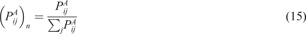
Nevertheless, the association analysis does not capture all possible combinations of features, as there is a minimum frequency for detection (the lowest detected frequency was 1180 records) below which the combination is considered insignificant. The limited ability of the association analysis to detect all possible combinations leaves combinations with a frequency lower than 1180 records without a corresponding frequency. Consequently, it restricts the use of equation (10) to predict the probability of all possible combinations. To overcome the association analysis’s prescribed deficiency, we developed a regression model based on the combinations identified by the association analysis. Then the pairwise probabilities for each pair of states in S were calculated using the developed regression model. The calculated pairwise probabilities were populated into a 35 × 35 matrix denoted as $P^{'}$ , in which each element $P_{i j}^{'} = P r (j | i)$ and $P_{i j}^{'} = P_{j i}^{'}$ .

$P^{'}$ does not have the shape of P depicted in equations (8) and (9). In this context, it is necessary to emphasize that the identified actions are means for communication with the MDP agent based on the rationale used to develop the model. These actions do not have a real-life manifestation. For that reason, the analysis of existing data co-occurrence will not yield a probability matrix similar to those in equations (8) and (9). Instead, further operations are required to develop a transition probability matrix for each of the actions, i.e. F, B, W, and E, as described in the following subsections.

Forming P^F

The elements of P^F are calculated as per equation (11).

P_{ij}^{F} = {\begin{matrix} 0 i f (i, j b e l o n g t o t h e s a m e s u b s e t) O R (j i s n o t i n D e s t (i, F)) \\ P_{ij}^{'} o t h e r w i s e \end{matrix}

(11)

Forming P^B and P^B1

Considering the moving logic of B and B1, it is possible to write:

P^{B} = P^{B 1} = P^{F t}

(12)

Forming P^B2, P^B3, P^B4, and P^B5

The elements of P^B2, P^B3, P^B4, and P^B5 adhere to equation (13).

P_{ij}^{Bk} = {\begin{matrix} 0 i f (P_{ij}^{F} \neq 0) O R (i, j b e l o n g t o t h e s a m e s u b s e t) O R (j i s n o t i n D e s t (i, B k)) \\ P_{ij}^{'} o t h e r w i s e \end{matrix}

(13)

where

k ϵ {2, 3, 4, 5}

Forming P^W

Based on the design problem’s definition, it is not logical to have two alternatives from the same subset. Consequently, we cannot use the developed pairwise probabilities to calculate the probabilities of P^W’s elements. Thus, we use conditional probabilities as follows.

P_{ij}^{F} = {\begin{matrix} 0 i f (i, j b e l o n g t o d i f f e r e n t s u b s e t s) O R (j = i) \\ P_{ij}^{W} = \Pr (j | i) = o c c_{i} \times o c c_{j} o t h e r w i s e \end{matrix}

(14)

Where occ_i is the probability of choosing alternative i and given in Table 3, and

P_{ji}^{W} = P_{ij}^{W}

Table 3.

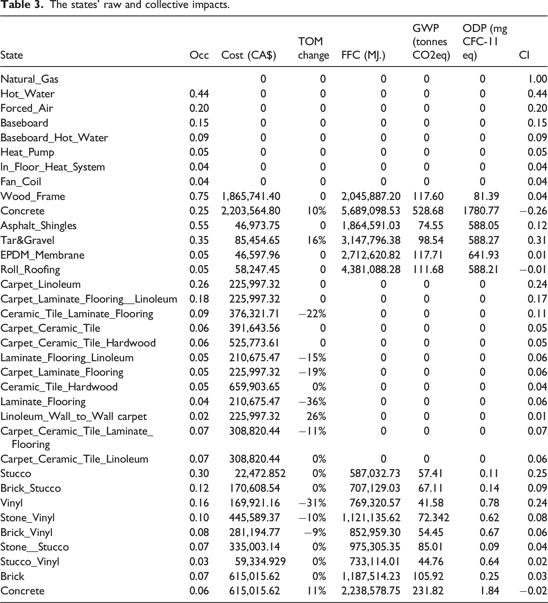
The states' raw and collective impacts.

State	Occ	Cost (CA$)	TOM change	FFC (MJ.)	GWP (tonnes CO2eq)	ODP (mg CFC-11 eq)	CI
Natural_Gas		0	0	0	0	0	1.00
Hot_Water	0.44	0	0	0	0	0	0.44
Forced_Air	0.20	0	0	0	0	0	0.20
Baseboard	0.15	0	0	0	0	0	0.15
Baseboard_Hot_Water	0.09	0	0	0	0	0	0.09
Heat_Pump	0.05	0	0	0	0	0	0.05
ln_Floor_Heat_System	0.04	0	0	0	0	0	0.04
Fan_Coil	0.04	0	0	0	0	0	0.04
Wood_Frame	0.75	1,865,741.40	0	2,045,887.20	117.60	81.39	0.04
Concrete	0.25	2,203,564.80	10%	5,689,098.53	528.68	1780.77	−0.26
Asphalt_Shingles	0.55	46,973.75	0	1,864,591.03	74.55	588.05	0.12
Tar&Gravel	0.35	85,454.65	16%	3,147,796.38	98.54	588.27	0.31
EPDM_Membrane	0.05	46,597.96	0	2,712,620.82	117.71	641.93	0.01
Roll_Roofing	0.05	58,247.45	0	4,381,088.28	111.68	588.21	−0.01
Carpet_Linoleum	0.26	225,997.32	0	0	0	0	0.24
Carpet_Laminate_Flooring__Linoleum	0.18	225,997.32	0	0	0	0	0.17
Ceramic_Tile_Laminate_Flooring	0.09	376,321.71	−22%	0	0	0	0.11
Carpet_Ceramic_Tile	0.06	391,643.56	0	0	0	0	0.05
Carpet_Ceramic_Tile_Hardwood	0.06	525,773.61	0	0	0	0	0.05
Laminate_Flooring_Linoleum	0.05	210,675.47	−15%	0	0	0	0.06
Carpet_Laminate_Flooring	0.05	225,997.32	−19%	0	0	0	0.06
Ceramic_Tile_Hardwood	0.05	659,903.65	0%	0	0	0	0.04
Laminate_Flooring	0.04	210,675.47	−36%	0	0	0	0.06
Linoleum_Wall_to_Wall carpet	0.02	225,997.32	26%	0	0	0	0.01
Carpet_Ceramic_Tile_Laminate_Flooring	0.07	308,820.44	−11%	0	0	0	0.07
Carpet_Ceramic_Tile_Linoleum	0.07	308,820.44	0%	0	0	0	0.06
Stucco	0.30	22,472.852	0%	587,032.73	57.41	0.11	0.25
Brick_Stucco	0.12	170,608.54	0%	707,129.03	67.11	0.14	0.09
Vinyl	0.16	169,921.16	−31%	769,320.57	41.58	0.78	0.24
Stone_Vinyl	0.10	445,589.37	−10%	1,121,135.62	72.342	0.62	0.08
Brick_Vinyl	0.08	281,194.77	−9%	852,959.30	54.45	0.67	0.06
Stone__Stucco	0.07	335,003.14	0%	975,305.35	85.01	0.09	0.04
Stucco_Vinyl	0.03	59,334.929	0%	733,114.01	44.76	0.64	0.02
Brick	0.07	615,015.62	0%	1,187,514.23	105.92	0.25	0.03
Concrete	0.06	615,015.62	11%	2,238,578.75	231.82	1.84	−0.02

Forming P^E

Action F is exclusive for the alternatives of ec, where $P_{ii}^{E} = 1$ if i in ec and $P_{ij}^{E} = 0$ otherwise.

The developed matrices are checked to ensure they are logical. In this context, we check for compliance with the actions' defined sequence and the mathematical logic, i.e. all values of a single row add up to 1. When checking for the mathematical logic, we may encounter one of the following cases:

• The sum of all probabilities on the same raw $(\sum_{j} P_{i j}^{A})$ is between 0 and 1, or $0 < \sum_{j} P_{i j}^{A} < 1$ , in such case, $P_{i j}^{A}$ is assigned a new value ${(P_{i j}^{A})}_{n}$ calculated which is its normalized value using the sum of all probabilities on the same raw, as shown in equation (15).

{(P_{i j}^{A})}_{n} = \frac{P_{i j}^{A}}{\sum_{j} P_{i j}^{A}}

(15)

• The sum of all probabilities on the same raw $(\sum_{j} P_{i j}^{A})$ equal 0, or $\sum_{j} P_{i j}^{A} = 0$ , in which, $P_{i i}^{A}$ is assigned a value of 1.

Once this process is complete, P_M1 and P_M2 are formed as per equations (8) and (9).

Figure 4 shows part of PF’s final form, where the reader can see how the moving forward logic is delivered to the agent.

Figure 4.

Partial depiction of P^F.

Figure 4 shows the first 10 states of S, where the numbers used to name the columns and rows are encoded as 0: Natural_Gas; 1:Hot_Water, 2:Forced_Air, 3:Baseboard, 4:Baseboard_Hot_Water, 5:Heat_Pump, 6:ln_Floor_Heat_System, 7:Fan_Coil, 8:Wood_Frame, 9:Concrete. In Figure 4, the reader can notice that, for example, since the agent cannot move from s₁= Natural_Gas to s₂ = Wood_Frame nor s₂ = Concrete, $P_{0,8}^{F} = P_{0,9}^{F} = 0$ . Action F will not lead to a value in the same subset. Thus, $P_{1,2}^{F} = \dots = P_{1,7}^{F} = 0$ .

It is worth noting that P’s development is based on the statistical occurrence observed in real-life data. By doing so, we are assuming the engineering and construction logics and their constraints are implicitly met.

Developing the reward matrix

We begin developing the reward matrix (R) by calculating each design alternative’s contribution to each performance metric or design alternatives' raw impacts. RS Means® database, Athena environmental database, and Tables A2 and A3 in²⁷ are used to calculate the raw impacts of the alternatives on construction cost, environmental metrics (FFC, GWP, and ODP), and TOM, respectively.

The collective impact of an alternative on the selected performance metrics is the agglomeration of its raw impacts. In this context, we can notice the following points.

• Each performance metric has its unit of measure, and, thus, we cannot add the raw impacts of a design alternative to find the corresponding reward.

• The desirable impact of the TOM has a different sign than the desirable impact on other performance metrics.

• The simple summation of the impact does not account for the effect of the industry’s familiarity with that alternative. To better understand this point, let us assume that alternative a is cheaper than other alternatives with the same category and is less harmful to the environment. However, local contractors do not have the required experience to dealing with a, which may lead to quality issues that reduce the gains from using alternative a.

To respond to these points, we define an alternative’s collective impact, as shown in equation (16).

C I_{i} = o c c_{i} \times (\frac{T O M_{i}}{\sum_{i} T O M_{i}} + 1 - \sum_{j} \frac{I_{i j}}{\sum_{i} I_{i j}})

(16)

where,

• $o c c_{i}$ is the occurrence of alternative i as per the association analysis;

• $T O M_{i}$ the change in the potential TOM of the building due to alternative i;

• I_ij is the impact of the design alternative i on performance metric j, where; and,

• ∑_i is performed on the alternatives that belong to the same subset.

Note that in equation (16), (i) the raw impacts of the design alternatives are normalized to create unitless numbers, (ii) the total reward was scaled up by adding 1 to all values before multiplying by the corresponding occurrence, which leads to more relatable values in the interval of ]−1, +1 [, and (iii) the familiarity of the industry with a given alternative was factored in by multiplying the sum of the normalized raw impacts by the alternative occurrence.

Table 3 shows the states’ raw and collective impacts where numbers are rounded up to two digits.

Note that the zero values in Table 3 are the results of the lack of information in the corresponding databases about some design alternatives, as discussed before.

R in the present work takes an identical shape as P, i.e. A×(S × S), and as in P, we distinguish between R_M1 as in equation (17) and R_M2 as in equation (18).

R_{M 1} = | \begin{matrix} R^{F} \\ R^{B} \\ \begin{matrix} R^{W} \\ R^{E} \end{matrix} \end{matrix} |

(17)

R_{M 1} = | \begin{matrix} R^{F} \\ \begin{matrix} R^{B 1} \\ R^{B 2} \\ \begin{matrix} R^{B 3} \\ R^{B 4} \\ R^{B 5} \end{matrix} \end{matrix} \\ \begin{matrix} R^{W} \\ R^{E} \end{matrix} \end{matrix} |

(18)

Populating R_M1 and R_M2 follows equations (19) to (23).

R_{ij}^{F} = {\begin{matrix} C I_{j} i f r_{i j}^{F} > 0 \\ - 1 o t h e r w i s e \end{matrix}

(19)

R_{ij}^{B} = R_{ij}^{B 1} = {\begin{matrix} - C I_{j} i f r_{i j}^{B} > 0 \\ - 1 o t h e r w i s e \end{matrix}

(20)

R_{ij}^{Bk} = {\begin{matrix} - C I_{i} - a v e r a g e r e w a r d o f e a c h s u b s e t b e t w e e n i a n d j s u b s e t s i f r_{i j}^{B k} > 0 \\ - 1 o t h e r w i s e \end{matrix}

(21)

R_{ij}^{W} = {\begin{matrix} C I_{j} - C I_{i} i f r_{i j}^{w} > 0 a n d i, j b e l o n g t o t h e s a m e s u b s e t \\ - 1 o t h e r w i s e \end{matrix}

(22)

R_{ij}^{E} = {\begin{matrix} C I_{i} i f i = j a n d i ϵ e c \\ - 1 o t h e r w i s e \end{matrix}

(23)

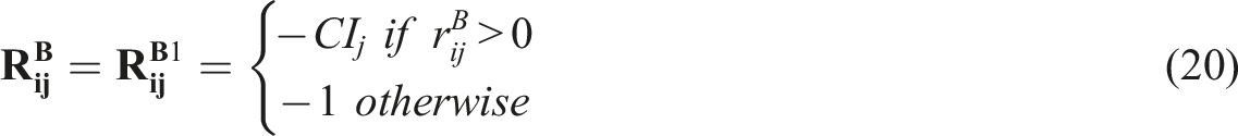
Figure 5 shows part of R^F matrix.

Figure 5.

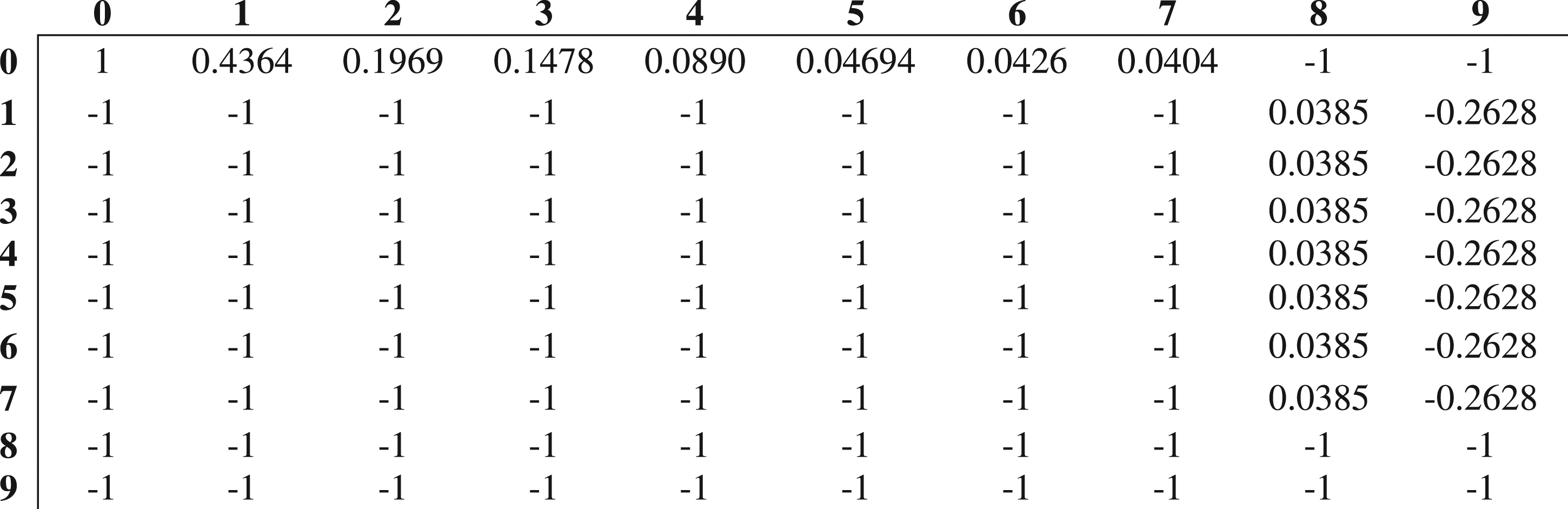
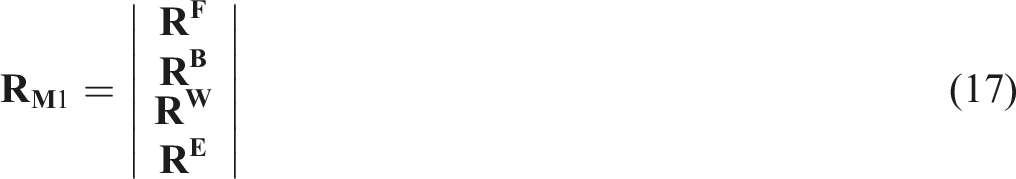
Partial depiction of R^F.

With the development of R_M1 and R_M2 is concluded, the next step is to run the developed models.

Results

Python’s MDP Toolbox was used to find the policy that maximizes the value shown in equation (6). Given that the primary motivation of this experiment is to further our understanding regarding best practices of RL implementation into the engineering design, we solved the identified models M1 and M2 using the subsequent algorithms:

• Finite-horizon backward induction (FHBI), in which the backward induction iterative procedure is used on a finite solution space with known states, as in the case of this research. The backward induction procedure begins at a terminal state and compute the values of previous states. The process is repeated until an optimal policy is found.²⁸

• Value iteration (VI); which consecutively approximates the value vector until it converges into the optimal value that corresponds to the optimal policy.²⁸

• Policy-iteration (PI), where a sequence of policies is formed, in which the value of a succeeding policy is greater than its immediate predecessor, until an optimal policy is found.²⁸

• Modified policy-iteration (MPI), which combines the procedure of VI and PI to find an optimal solution.²⁸

• Q-learning, which considers the optimal policy at each decision point is the maximum possible function value at that point.

• Relative value iteration (RVI), which is similar to the VI algorithm in terms of process, but the value after each interaction is normalized according to a reference state, which create the “relative” iteration.²⁹

• Gauss-Seidel value iteration (GSVI), which is a variation of VI, in which the value of the calculated state is used in immediate succeeding step.³⁰

We explored different parameters during the runs, including changing the discount factor (the experimental runs are explained in the next section). Table 4 shows each state’s optimal action as suggested by each algorithm per the model and a discount factor of 0.4.

Table 4.

The results of solving the developed models.

Subset	State	FHBI		PI		MPI		Q-learning		RVI		VI		GSVI
Subset	State	M1	M2	M1	M2	M1	M2	M1	M2	M1	M2	M1	M2	M1	M2
hs	Natural_Gas	F	F	F	F	F	F	F	F	F	F	F	F	F	F
ht	Hot_Water	F	F	F	F	F	F	F	F	F	F	F	F	F	F
	Forced_Air	W	W	F	F	F	F	B	F	F	F	F	F	F	F
	Baseboard	W	W	W	W	W	W	F	W	F	F	W	W	W	W
	Baseboard_Hot_Water	W	W	W	W	W	W	W	W	F	F	W	W	W	W
	Heat_Pump	W	W	W	W	W	W	F	W	F	F	W	W	W	W
	ln_Floor_Heat_System	W	W	W	W	W	W	W	W	F	F	W	W	W	W
	Fan_Coil	W	W	W	W	W	W	W	W	F	F	W	W	W	W
ct	Wood_Frame	F	F	F	F	F	F	F	F	F	F	F	F	F	F
ct	Concrete	W	W	W	W	W	W	F	B1	F	F	W	W	W	W
rt	Asphalt_Shingles	F	F	F	F	F	F	F	F	F	F	F	F	F	F
	Tar&Gravel	F	F	F	F	F	F	F	F	F	F	F	F	F	F
	EPDM_Membrane	W	W	W	W	W	W	F	F	F	F	W	W	W	W
	Roll_Roofing	W	W	W	W	W	W	W	F	F	F	W	W	W	W
fl	Carpet_Linoleum	F	F	F	F	F	F	F	F	F	F	F	F	F	F
	Carpet_Laminate_Flooring_Linoleum	F	F	F	F	F	F	F	F	F	F	F	F	F	F
	Ceramic_Tile_Laminate_Flooring	F	F	F	F	F	F	F	F	F	F	F	F	F	F
	Carpet_Ceramic_Tile	F	F	F	F	F	F	F	F	F	F	F	F	F	F
	Carpet_Ceramic_Tile_Hardwood	F	F	F	F	F	F	W	F	F	F	F	F	F	F
	Laminate_Flooring_Linoleum	F	F	F	F	F	F	F	F	F	F	F	F	F	F
	Carpet_Laminate_Flooring	F	F	F	F	F	F	F	F	F	F	F	F	F	F
	Ceramic_Tile_Hardwood	F	F	F	F	F	F	F	F	F	F	F	F	F	F
	Laminate_Flooring	F	F	F	F	F	F	F	F	F	F	F	F	F	F
	Linoleum_Wall_to_Wall carpet	F	F	F	F	F	F	F	F	F	F	F	F	F	F
	Carpet_Ceramic_Tile_Laminate_Flooring	F	F	F	F	F	F	F	F	F	F	F	F	F	F
	Carpet_Ceramic_Tile_Linoleum	F	F	F	F	F	F	F	F	F	F	F	F	F	F
ec	Stucco	E	E	E	E	E	E	E	E	E	E	E	E	E	E
	Brick_Stucco	E	E	E	E	E	E	E	E	W	W	E	E	E	E
	Vinyl	E	E	E	E	E	E	E	E	W	W	E	E	E	E
	Stone_Vinyl	E	E	E	E	E	E	E	E	W	W	E	E	E	E
	Brick_Vinyl	E	E	E	E	E	E	W	E	W	W	E	E	E	E
	Stone_Stucco	E	E	W	W	W	W	W	E	W	W	W	W	W	W
	Stucco_Vinyl	W	W	W	W	W	W	W	W	W	W	W	W	W	W
	Brick	E	E	W	W	W	W	W	W	W	W	W	W	W	W
	Concrete	W	W	W	W	W	W	B	B1	W	W	W	W	W	W

In Table 4, each algorithm assigned an action to each design alternative based on the used model. For instance, the Q-learning algorithm assigned concrete, as a construction type, F when using M1 to solve the design problem and B1 when using M2. The policies shown in Table 4 guide the agent to navigate its way through the states. As mentioned earlier, A state associated with action F is a state in the optimum policy. The same goes for a state in ec that is associated with action E. When the agent encounters a state associated with action W, it seeks to change its choice to another design alternative that belongs to the current state’s subset. When the action associated with a state is B (or B1), it is more rewarding that the agent goes back to select a state from the subset that immediately preceded the current state.

As for designers, their choice of alternatives is from those marked with actions F and E as those combined maximize the desirable influence on the selection criteria, i.e. cost, TOM, FFC, GWP, and ODP. For instance, based on Table 4, using natural_gas as a heating source, hot_water as heating type, wood_frame as a construction type, asphalt_shingles as a roof type, carpet_linoleum as a flooring material, and stucco as an exterior cladding maximizes the desired influence on the considered criteria. Note that natural_gas, hot_water, wood_frame, asphalt_shingles, and carpet_linoleum have an action F associated with them, and stucco has an action E associated with it, regardless of the used solving algorithm.

It is worth mentioning that the suggested policies are also detectable in the dataset. For instance, the previously mentioned policy, i.e. <natural_gas, hot_water, wood_frame, asphalt_shingles, carpet_linoleum, stucco>, appears 1251 times in the dataset, which indicates that the model provides realistic suggestions that match what is seen in real life.

Discussion

Results discussion

Solving both models, i.e. M1 and M2, shows very comparable results with a few exceptions, indicating that restricting the agent’s movement did not lead to a drastic change in the outcomes. Using the Q-learning algorithm resulted in considerable differences between the outcomes of the two models, M1 and M2, while the rest of the algorithms show no difference.

Furthermore, design alternatives that belong to fl seem to have less influence on the overall reward given that all the states of this subset are assigned action F regardless of the solving algorithm. A reason for that may be ignoring their environmental impact, which renders them less influential.

As for the used algorithms, RVI seems to be the least sensitive to this experiment’s input. As the reader can see in Table 4, RVI assigned action F to almost all the states in both models, which is unrealistic in this experiment as the states cannot be equally influential.

To further understand the influence of the model’s components, we sought answers to the following questions:

• How sensitive are the outcomes to the discount factor?

• How can the reward assignment change the outcomes?

We ran the models while changing the discount factor between 0.1 and 0.9 with 0.1 increments to pursue the first question. The rate of change at a discount factor i is the number of states that witnessed a change in the assigned action, when changing the discount factor from i+1 to i, divided by 35 (the total number of states). The rate of change is shown in Figure 6 for M1 and in Figure 7 for M2. Finite-horizon backward induction and RVI outcomes do not change regardless of the discount factor value. Conversely, Q-learning shows the most considerable sensitivity to the discount factor’s changes, followed by the MPI algorithm. PI, GSVI, and VI show similar sensitivity to the discount factor but less than Q-learning and MPI.

Figure 6.

The sensitivity of M1 optimum policy to the changes in the discount factor.

Figure 7.

The sensitivity of M2 optimum policy to the changes in the discount factor.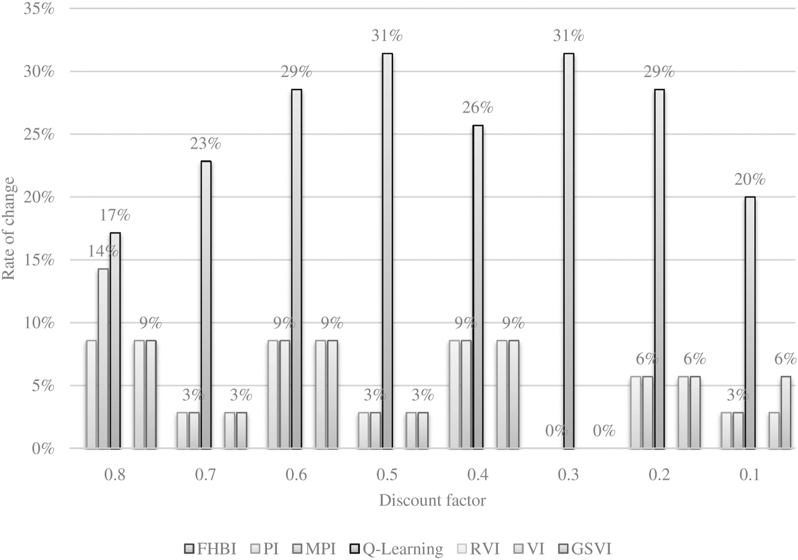

As for the second question, let us begin by clarifying what we mean by reward assignment. In equations (19) to (23), there are two types of values; a calculated value and a single value assigned to matrices elements other than those of calculated values, i.e. −1. The reward assignment question is concerned with the latter. In this context, we noticed that it is crucial to assign a maximum penalty (a negative reward) more significant in the absolute value than any calculated penalty to discourage specific actions from certain states. Given such actions, a neutral value, i.e. a value of (0), allows the agent to be lax with its selections. The same goes for rewarding terminal, i.e. ec, and starting, i.e. hs, states with maximum reward. As long as it is more significant than all calculated penalties in absolute terms, the penalty value has virtually no influence on the outcomes.

On the other hand, the maximum reward can significantly affect the outcomes. A large terminal or starting reward led to indifference in the state selection in between. We found that a value of (1) is suitable for the problem in the present research as all calculated rewards (and penalties) are in the interval of [−1, 1]. Building on this observation, the terminal and starting states, i.e. ec and hs elements, are best to be assigned a value proportional to the calculated values, just marginally larger than the largest calculated reward.

Reflection on the results

The results reported in this paper provide several insights that help better understand the role of machines in engineering design in the AEC industry.

The use of RL represented in MDP shows that it requires considerably fewer iterations (convergence occurred within the first 200 iterations) compared to the conventional approach, i.e. using brute computation force. This comes to importance in larger design problems where the number of design decisions is thousands. BuHamdan et al. ³¹ noted the importance of developing a generative system that supports several building systems’ design. However, as the number of building systems considered for design increases, the computation effort needed to conduct an analysis, like what is described in this work, increases. To maintain the developed system’s efficiency, we need to reduce the space of feasible solutions without compromising optimality. Here comes the use of MDP handy. It provides the opportunity to quickly assess all possible alternatives and transfer the high-ranked ones to the generative system to perform the detailed analysis and generate the optimum design accordingly.

Another essential advantage of using RL is the possibility of knowledge transfer. Once the model is trained, the knowledge acquired can be used to solve similar problems, provided the context remains the same in terms of possible states and their corresponding probabilities and rewards. This reduces the model development and training time and increases engineering design efficiency. Additionally, as the reader can observe, the model itself is transparent and permits designers to convey as much input as they see necessary. The designer can convey any engineering or construction requirement to model and monitor its execution, unlike other AI techniques in which a blackbox controls the model behaviour.

It is also important to address the validity of the suggested policies, i.e. design values. The logical soundness of the solution that results from using MDP modelling to support design endeavors comes down to setting the movement of the agents between states. Design logic and users and clients' preferences are communicated to MDP agents through a combination of actions, rewards, and probabilities. When it is illogical to move from State A to State B, then there would be no action that connects them, or the move is assigned a transitional probability of zero (0). Both approaches will deter the agent from making a move, and, consequently, preventing it from suggesting illogical solutions.

Research limitations

While the results presented in this paper show that RL can efficiently aid engineering design endeavours in the AEC industry, it is essential to acknowledge that these findings should be approached with the following limitations in mind.

• Despite that the data used to populate the present research model are real-life data, they come from a single market, Edmonton. Therefore, it reflects the preferences of Edmontonians and the design practices in that region. While the structure can support the design of condominiums in other places, the exact model, the transition and reward matrices, cannot.

• Even though the starting size of the used dataset (some 64,000 records) is relatively large, the data used to develop the regression model that is later used to assess the states' pairwise probabilities is relatively small. Nevertheless, as the reader notices in the paper, the pairwise probabilities are used as a primary assessment tool. They are later normalized and adjusted to meet the transition matrix requirements.

• The dependence on the statistical co-occurrence to develop the transitional probabilities within the MDP model might shift the selection process toward existing and commonly used combinations, consequently, limiting the agent from suggesting novel solutions. However, we see the bias resulting from the co-occurrence analysis is balanced by reward assignments, which is partially independent of the dataset bias. Given the nature of selection in MDP, which depends on two aspects, the probability and the possible reward, the potential reward is the counterbalance for the bias that may exist in the transitional probabilities. In other words, if a design feature is commonly used in the existing dataset, the agent more likely to select that feature. Nevertheless, if that feature has a negative impact on the desired performance metrics, then the proposed MDP model will penalize that selection. The authors also see the statistical co-occurrence a practical mean to transfer the general wisdom of designers into the system and convey the construction logic and building codes.

Conclusion

While design in the AEC continues to be a creative activity, approaching the design problem from a perspective of decision-making science has remarkable potentials that manifest in the delivery of appealing and sustainable structures. The decision-making approach brings many opportunities, including AI techniques, to help generate and optimize the design process’s deliverables. Indeed, AI offers computational power accompanied by the knowledge acquired from real-life data to help designers evaluate many design alternatives and choose those that maximize the gain. Such combination, i.e. data knowledge and computation power, comes to extreme importance amid the mounting pressure on the AEC industry players to deliver economic, environmentally friendly, and socially considerate structures.

This paper’s experimental research presents a strong case for implementing AI, particularly RL, to support the AEC industry’s design endeavors. It demonstrates the developed models' effectiveness and efficiency to find combinations that lower cost and environmental impact while maintaining a high desirability. The RL models’ transparency increases the credibility of the outcomes and removes the hurdles of full human-machine integration in design practices. However, the present research’s findings and observations must be approached with its limitation in mind, primarily, the assumptions concerning the rewards assessment and the sample size used to develop the regression model. While these issues may limit the wide use of the model, they can be easily overcome by changing the databases used to develop those components.

Although the present research uses a defined design problem for testing, the outlined process can be replicated and applied to other design problems, where data permits; after all, RL remains a technique that acquires knowledge through data.

Footnotes

Acknowledgements

The authors would like to thank the REALTOR® Association of Edmonton for providing the data to conduct the present research.

Declaration of conflicting interests

The author(s) declared no potential conflicts of interest with respect to the research, authorship, and/or publication of this article.

Funding

The author(s) received no financial support for the research, authorship, and/or publication of this article.

Data availability

Some or all data, models, or code used during the study were provided by a third party. Direct requests for these materials may be made to the provider as indicated in the Acknowledgements.

ORCID iD

Samer BuHamdan

References

Cheung

Scanlan

Wong

, et al. Application of value-driven design to commercial aeroEngine systems. J Aircr 2012; 49: 688–702.

Miller

Yukish

Simpson

. Design as a sequential decision process. Struct Multidiscip Optim 2018; 57: 305–324.

BuHamdan

Alwisy

Barkokebas

, et al. A multi-criteria lifecycle assessment framework for evaluating building systems design. J Build Eng 2019; 23: 388–402. DOI: 10.1016/j.jobe.2019.02.010.

BuHamdan

. A Framework for multi-criteria lifecycle assessment of building systems in the construction industry. Edmonton, Alberta, Canada: University of Alberta, 2018.

BuHamdan

Alwisy

Bouferguene

, et al. The application of multi-attribute utility theory for a market share-based design evaluation. Int J Hous Mark Anal 2019; 12: 985–1003.

Park

Kwon

Shin

, et al. Cost and CO2 emission optimization of steel reinforced concrete columns in high-rise buildings. Energies 2013; 6: 5609–5624.

Yepes

Martí

García-Segura

. Cost and CO2 emission optimization of precast–prestressed concrete U-beam road bridges by a hybrid glowworm swarm algorithm. Autom Constr 2015; 49: 123–134.

Russell-Smith

Lepech

Fruchter

, et al. Sustainable target value design: integrating life cycle assessment and target value design to improve building energy and environmental performance. J Clean Prod 2015; 88: 43–51.

Curran

, 2010 Value-driven design and operational value. Encyclopedia Aerospace Eng. Epub ahead of print 15 December 2010. DOI: doi:10.1002/9780470686652.eae553.

10.

Schümmer

Haake

Stark

. Beyond rational design patterns. In: 19th European Conference on Pattern Languages of Programs, EuroPLoP 2014. Faculty of Mathematics and Computer Science, Fern Universität in Hagen, Universitätsstr. 1, Hagen, 58084, Germany, 2014. Association for Computing Machinery. Epub ahead of print 2014. DOI: 10.1145/2721956.2721984.

11.

Collopy

Hollingsworth

. Value-driven design. J Aircr 2011; 48: 749–759.

12.

Collopy

. A research agenda for the coming renaissance in systems engineering. In: 50th AIAA Aerospace Sciences Meeting Including the New Horizons Forum and Aerospace Exposition, Nashville, Tennessee, 09–12 January 2012, 2012, p. 799.

13.

Alwisy

Barkokebas

Hamdan

, et al. Energy-based target cost modelling for construction projects. J Build Eng 2018; 20: 387–399.

14.

BuHamdan

Alwisy

Bouferguene

. Explore the application of reinforced learning to support decision making during the design phase in the construction industry. Proced Manuf 2020; 42: 181–187.

15.

Niese

Kana

Singer

. Ship design evaluation subject to carbon emission policymaking using a Markov decision process framework. Ocean Eng 2015; 106: 371–385.

16.

Niese

ND.

Life Cycle Evaluation under Uncertain Environmental Policies Using a Ship-Centric Markov Decision Process Framework. Ann Arbor, Michigan, United States: University of Michigan, 2012, http://deepblue.lib.umich.edu/handle/2027.42/96130 (accessed 27 January 2021).

17.

Mckenney

TA.

An early-stage set-based design reduction decision support framework utilizing design space mapping and a graph theoretic Markov decision process formulation. Ann Arbor, Michigan, United States: University of Michigan, 2013, http://deepblue.lib.umich.edu/handle/2027.42/102464 (accessed 27 January 2021).

18.

Ororbia

Warn

. Structural design synthesis through a sequential decision process. In: Volume 9: 40th Computers and Information in Engineering Conference (CIE), St.Louis, Missoury, United States, 17–19 August 2020, American Society of Mechanical Engineers, 2020. Epub ahead of print 17 August 2020. DOI: 10.1115/DETC2020-22647.

19.

Chhabra

JPS

Warn

. A method for model selection using reinforcement learning when viewing design as a sequential decision process. Struct Multidiscip Optim 2019; 59: 1521–1542.

20.

Karan

Asadi

. Intelligent designer: a computational approach to automating design of windows in buildings. Autom Constr 2019; 102: 160–169.

21.

Shabestari

Herzog

Bender

. A survey on the applications of machine learning in the early phases of product development. Proc Des Soc Int Conf Eng Des 2019; 1: 2437–2446.

22.

Chatterjee

Majumdar

Henzinger

. Markov decision processes with multiple objectives. In: Lecture Notes in Computer Science (including subseries Lecture Notes in Artificial Intelligence and Lecture Notes in Bioinformatics). Berlin, Heidelberg: Springer, pp. 325–336.

23.

Sutton

Barto

. Reinforcement learning: an introduction. Cambridge, Massachusetts; London, England: The MIT Press, 2018, http://incompleteideas.net/book/first/ebook/the-book.html (accessed 21 December 2020).

24.

Littman

. Value-function reinforcement learning in Markov games. Cogn Syst Res 2001; 2: 55–66.

25.

Wiering

De Jong

. Computing optimal stationary policies for multi-objective markov decision processes. In: 2007 IEEE International Symposium on Approximate Dynamic Programming and Reinforcement Learning, Honolulu, HI, USA, 1–5 April 2007. IEEE, 2007, pp. 158–165.

26.

Fard

Pineau

. Non-deterministic policies in Markovian decision processes, 2011.

27.

BuHamdan

Alwisy

Bouferguene

. Drivers of housing purchasing decisions: a data-driven analysis. Int J Hous Mark Anal 2021; 14: 97–123. DOI: 10.1108/IJHMA-02-2020-0018.

28.

Kallenberg

Markov decision processes. Lecture Notes. Leiden, Netherlands: University of Leiden, 2011, https://www.math.leidenuniv.nl/∼kallenberg/Lecture-notes-MDP.pdf.

29.

Gupta

Jain

Glynn

. An empirical algorithm for relative value iteration for average-cost mdps. In: 2015 54th IEEE Conference on Decision and Control (CDC), Osaka, Japan, 15–18 December 2015, IEEE, 2015, pp. 5079–5084.

30.

Blackledget

. Iterative methods of solution. In: Digital signal processing. Burlington: Elsevier; 2006, pp. 237–254.

31.

BuHamdan

Alwisy

Bouferguene

. Generative systems in the architecture, engineering and construction industry: a systematic review and analysis. Int J Architectural Comput 2021; 19: 226–249. DOI: 10.1177/1478077120934126.

The use of reinforced learning to support multidisciplinary design in the AEC industry: Assessing the utilization of Markov Decision Process

Abstract

Keywords

Introduction

Methods and materials

Mathematical background- MDP model

The design problem

The design problem from a decision-making perspective

Developing the MDP model for the design problem

Define the model’s states

Define the model’s actions

Developing the transition probability matrix

Forming P F

Forming P B and P B1

Forming P B2 , P B3 , P B4 , and P B5

Forming P W

Forming P E

Developing the reward matrix

Results

Discussion

Results discussion

Reflection on the results

Research limitations

Conclusion

Footnotes

Acknowledgements

Declaration of conflicting interests

Funding

Data availability

ORCID iD

References

Forming P^F

Forming P^B and P^B1

Forming P^B2, P^B3, P^B4, and P^B5

Forming P^W

Forming P^E