Solving planning problems with evolutionary computation

Abstract

Evolutionary design (ED) is a strategy that makes use of computational power to couple generative techniques with evaluation methods, to put forward designs that are better with each iteration. In this research, we present a representation scheme for solving spatial layout problems that is simple to implement as well as extend. The mechanisms for evaluation and mutation are defined and also shown to be extendable. Ultimately, the topic explored here is the ways in which ED and computation can enhance our design thinking and how computers can provide the background to new design processes and workflows.

Keywords

evolutionary design evolutionary thinking genetic algorithms spatial planning problem solving

Introduction

Evolutionary computation (EC) is a field based on the idea that the process of biological evolution can be abstracted as a useful tool to solve artificial problems.

Many other forms of generative design methods have gained popularity in recent times including topological optimisation, artificial neural networks and parametric modelling. Wu et al.¹ give a summary of the advances in the broader category of generative design This research is focussed on evolutionary methods and highlights the features that make it appealing in the design space (as opposed to only the space of optimisation suited for many engineering problems).

Biological evolution has led to an incredible variety of life forms all adapted to the local conditions they face. Using evolution as the overarching metaphor makes the algorithm and associated heuristics and representations more intuitively understood than most other algorithms. As a form of stochastic optimisation, random sampling is key to traversing large solution spaces, for which exhaustive searching is not an option. Biological evolution makes use of both random mutations as well as genetic inheritance, the combination direct the process towards optimal outcomes – organisms better adapted for a given environment. Evolutionary design (ED) makes use of EC for the purposes of solving design problems. Design problems include the generation of form, space planning and optimisation. The advantages that ED brings to the table include the following:

1. An intuitive was of describing the workflow, or process, which sees the solution as something generated – contrast this with an algorithm that is only about optimisation.

2. The solution does not have to be described, only the evaluation rules, so a population of solutions are present at every iterative step (even though they might not contain the globally best solution). This does mean that no matter when the process is terminated, there is always a result given, which allows for interaction throughout the process or changing parameters and initial assumptions.

3. It presents a system that allows for an arbitrary number of heuristics to be used and these can interplay in different ways, for example, one set of heuristics can have a greater influence on a particular lineage of solutions which emphasise some characteristics. For example, one set of heuristics might emphasise symmetry and aesthetics, while another might have a greater emphasis on functionality or reducing waste. It is straightforward to code niches can be defined, to allow a variety of solutions to be generated and evolved.

4. The process is scalable as the most computational expensive parts (evaluating fitness) can be run in parallel. The problem solving can therefore be spread over multiple computational processors.

5. Unexpected results occur quite frequently (as random mutations generate novel results) and this in turn can stimulate the creative process.

What is equally interesting to the practical application of ED, is the way in which taking this lens can direct ‘design thinking’. Evolutionary thinking brings with it a rich nomenclature for concepts that are abstract and emerge at different scales. Delanda² believes that the use of genetic algorithms brings to design knowledge philosophical thinking which include the following:

1. Populational thinking – working with populations of solutions and understanding the trade-offs that take place when evaluating fitness. For example, it can be seen when running an EC simulation how even small advantages lead to Pareto distributions in the fitness of a population.

2. Topological thinking – articulating the way in which elements are connected, in biology the concept is that of a body-plan which corresponds to lineage, that is, primates, a category of mammal which shares an ancestry with reptiles all share the inherited body plan of a vertebral column (or spine). Life forms that are further on the phylogenetic tree have less resemblance that those that are closer.

The last of Delanda’s ‘thinking’ that of ‘intensive thinking’ (working with materially distributed quantities such as temperature or pressure) is of less relevance to this research. Researchers of note, working in the field of ED include Bentley³ with the text An Introduction to ED by Computer which gave a survey of both the techniques and strategies of EC and several applications of ED in industrial design. Janssen⁴ demonstrates the generation and evolution of housing through evolutionary algorithms in an implemented software application. In the field of generating artificial life and Sims⁵ pioneered some of the earliest work evolving generated ‘life’ based on their ability to move in a virtual world as creatures would in the physical world.

In applying ED to spatial planning, Homayouni⁶ and Verma and Thakur⁷ each give different representations for floor plan evolution, the former taking a two-step approach, first in generating rooms and then arranging them, and the latter by limiting the solution space by the type of room and the constraint that they fill a rectangular boundary. Matthews et al.⁸ apply genetic algorithms to land-use planning, Hu and Wang (2002) use GAs for facilities layout planning. Many examples of genetic algorithms for engineering optimisation exist and enumerating them would require a dedicated review. One example of particular note, came from Keane and Brown⁹ who used GAs in the design of a satellite boom, the case-study is widely cited, for the unusual design that emerged from the algorithm, too complex to be human-designed as the particularly pronounced increase in efficiency of the solution when compared to the initial design.

In designing an implementation of an evolutionary system, key elements which need to be decided upon include the design of the representation used for the solution space; the evaluation mechanism for determining fitness; the way in which the user will interact with the system; the genetic operations which may include crossover and mutation; and the mapping from genotype to phenotype. To make it clear as to how all these elements work together to form an ED system, the canonical genetic algorithm will be summarised in the next section.

Genetic algorithms

The ‘Genetic Algorithm’ is the most well known of the canonical approaches to EC. While Alan Turing had described in 1950 the idea of evolutionary machines in his famous article ‘Computing machinery and intelligence’, it was Holland’s text ‘Adaptation in Natural and Artificial Systems’, which formalised and standardised the algorithm to the form in which it is used today. The steps of a genetic algorithm summarised from Sivandandam and Deepa (2008):

1. Initialise a population (either in a single list or in a set of niches).

2. Evaluate each member of the population against the fitness criteria.

3. Select a part of the population to live on while deleting the remainder.

4. Recombine to fill the population back to its maximum size.

5. Return to step two and repeat unless some termination criteria are met.

Figure 1 shows this as s flowchart diagram.

Figure 1.

The genetic algorithm.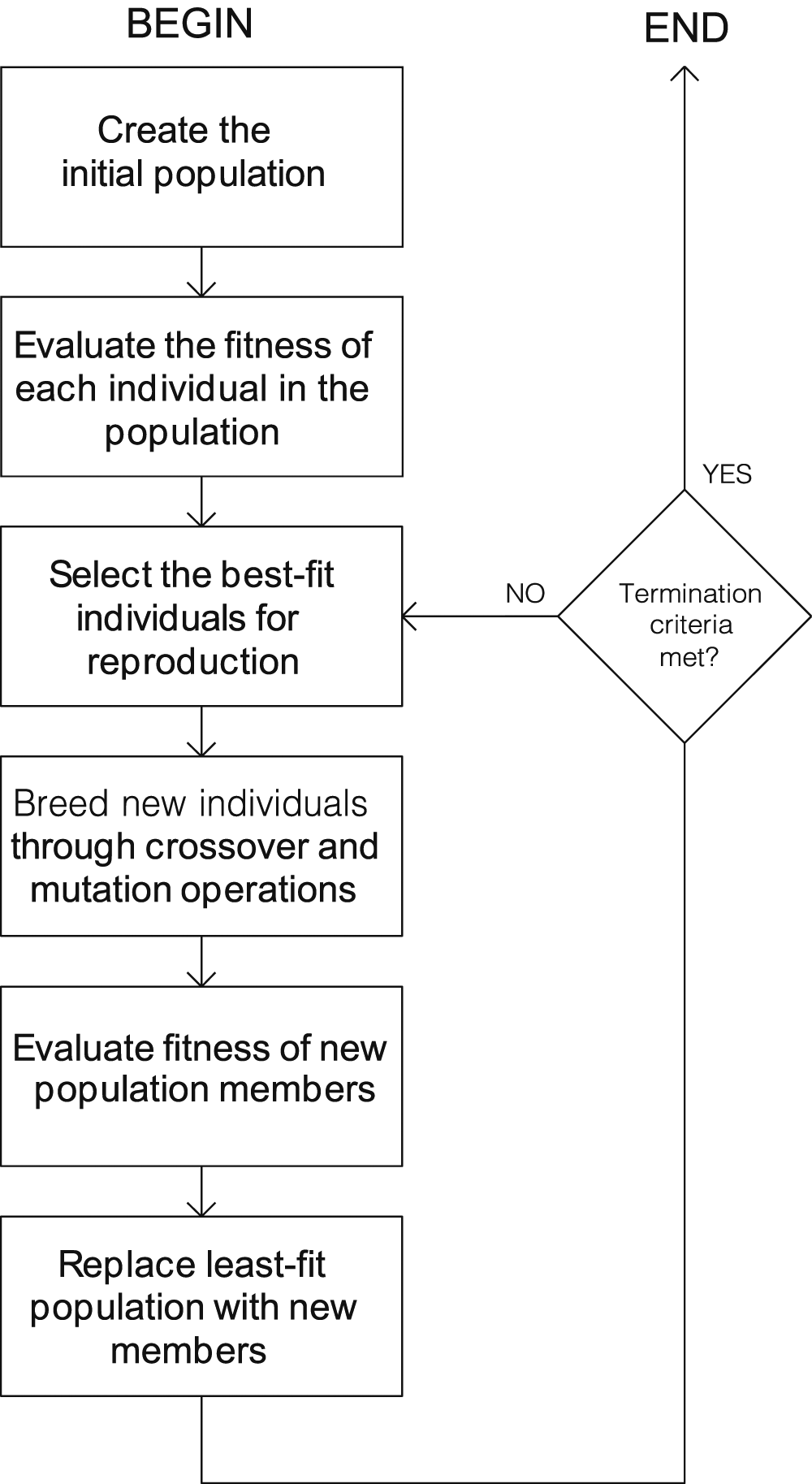

The initialisation of the population is typically performed randomly, though as with all search problems, the more that the problem is constrained, the smaller the search space becomes and less computationally expensive the process becomes. If there are any heuristics that tell us where optimal solutions may lie, these can have more population members added. This is also the stage for establishing niches and determining how many and what their maximum population allowed is. Niches help to keep variety in the system as members only compete with though within the same niche.

Evaluation requires an objective function, which itself might be composed of multiple subroutines that evaluate different criteria and are summed. It is quite common optimising one objective necessarily reduces performance in a different objective. For example, in the case of a house, imagine that two objectives that were being evolved were lighting performance and heating costs. Larger windows would lead to more light but would simultaneously be an area for heat loss or gain, reducing the efficiency of thermal performance. Therefore, part of using multi-objective criteria is also the weighting of different functions so that a solution that reaches acceptable levels across all criteria can be found.

Several techniques for selecting the fittest members of the population at each iteration. Sivandandam and Deepa (2008) describe six methods: roulette wheel selection, random selection, rank selection, tournament selection, Boltzmann selection and stochastic universal sampling. As a brief summary, the various selection processes perform better depending on factors such as the variance of fitness. If, for example, there is a great difference early on, a particular genetic line might converge and dominate the population as the chances for other members (that potentially would be stronger if they were allowed to continue to evolve) is so low that they are eliminated before given a chance. Using niches does have some mitigation on this effect.

Recombination is the way in new members of the population are created using the genetic encoding of the survivors of the last iteration. In biology, the two modes of reproduction are sexual and asexual with various subcategories. The most common representation for genetic algorithms is with bit string encoding where the genotype of the solution is described as a sequence of 1 s and 0 s. In such systems the most common means of creating new solutions is with crossover where part of one sequence are joined with another and mutation occurs as the random flipping of a bit from 0 to 1 or to 0. These representations tend to favours converging optimisation problems and for the implementation of this research a different approach was used as will be presented in the next section

The genetic algorithm approach is not without its critics, Skiena (2010) points out that GAs are not efficient for non-trivial problems and the genetic operators themselves, especially when abstracted to bit strings does not follow logical design. While these criticisms are targeted at EC, ED has different goals, as the aim is to find diverging solutions (as well as unexpected results) as opposed to optimisation. For optimisation problems, other approaches such as simulated annealing¹⁰ would be more efficient.

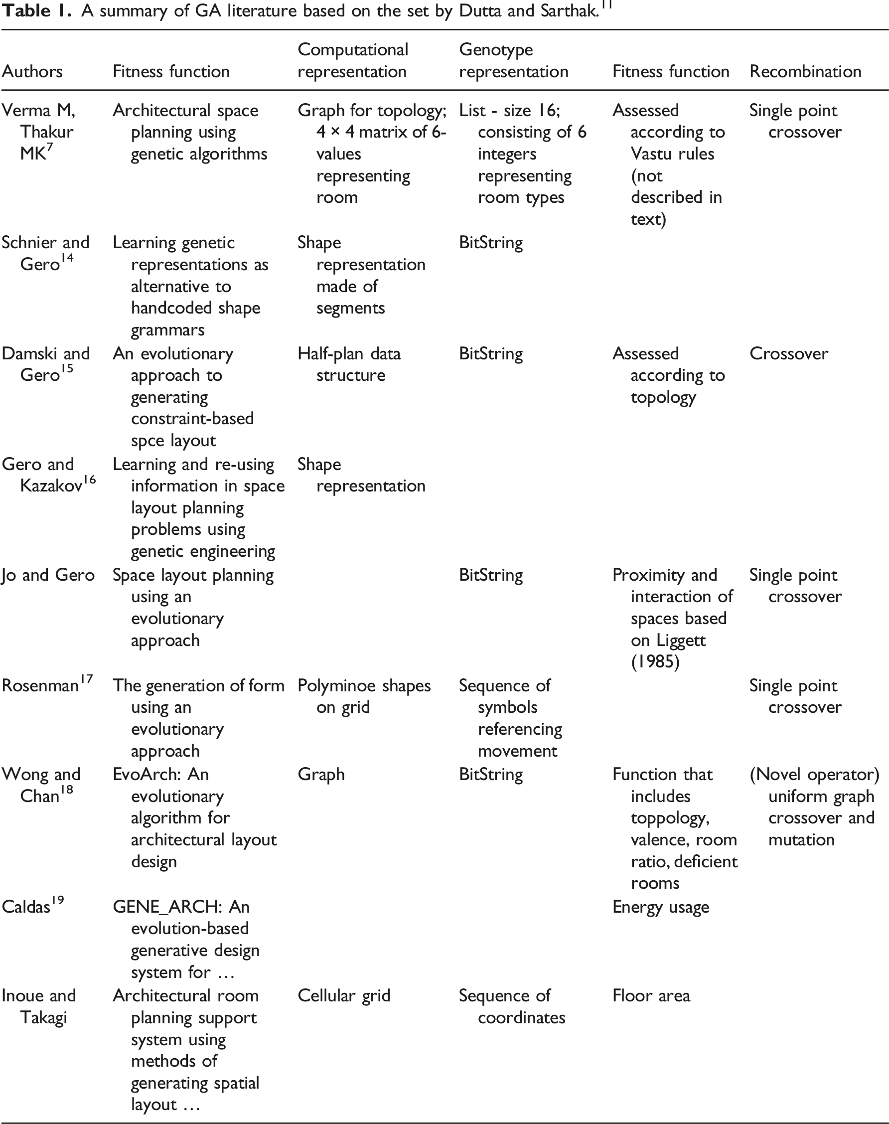
A review of spatial planning with evolutionary computation

Dutta and Sarthak¹¹ give a review of literature related to EC used for architectural space planning. The papers are classified by the following:

• The type of algorithm they use (the traditional Genetic Algorithm, Interactive Genetic Algorithm, Multi-Objective GA or other approaches such as Fuzzy Logic or Neural Networks).

• The input, output and constraints (topology shape grammars; cellular automaton seed; adjacency matrix; proximity matrix; relationship matrix; first order logic, etc.).

• Other notes such as whether energy is considered and what sample type was in use.

All of the literature from this review that were using genetic algorithms have been summarised in Table 1, but the criteria used instead are about the inner workings of the algorithm – the genotype representation, the computational representation, the fitness function and recombination operators. Figure 2

Table 1.

A summary of GA literature based on the set by Dutta and Sarthak.¹¹

Authors	Fitness function	Computational representation	Genotype representation	Fitness function	Recombination
Verma M, Thakur MK⁷	Architectural space planning using genetic algorithms	Graph for topology; 4 × 4 matrix of 6-values representing room	List - size 16; consisting of 6 integers representing room types	Assessed according to Vastu rules (not described in text)	Single point crossover
Schnier and Gero¹⁴	Learning genetic representations as alternative to handcoded shape grammars	Shape representation made of segments	BitString
Damski and Gero¹⁵	An evolutionary approach to generating constraint-based spce layout	Half-plan data structure	BitString	Assessed according to topology	Crossover
Gero and Kazakov¹⁶	Learning and re-using information in space layout planning problems using genetic engineering	Shape representation
Jo and Gero	Space layout planning using an evolutionary approach		BitString	Proximity and interaction of spaces based on Liggett (1985)	Single point crossover
Rosenman¹⁷	The generation of form using an evolutionary approach	Polyminoe shapes on grid	Sequence of symbols referencing movement		Single point crossover
Wong and Chan¹⁸	EvoArch: An evolutionary algorithm for architectural layout design	Graph	BitString	Function that includes toppology, valence, room ratio, deficient rooms	(Novel operator) uniform graph crossover and mutation
Caldas¹⁹	GENE_ARCH: An evolution-based generative design system for …			Energy usage
Inoue and Takagi	Architectural room planning support system using methods of generating spatial layout …	Cellular grid	Sequence of coordinates	Floor area

Figure 2.

Example of GP-systems and their genome.

Areas for development

As can be seen in the literature, most work uses single point crossover as a recombination operator – the merger of two bit-strings by splitting each one at a random point and taking a segment from each parent. While this has use in optimisation problems, the operation only converges towards a fitter solution if the parents are close enough in geno- and phenotype that the split brings about a similar offspring (else the recombination can be very different). While randomness is at the heart of EC, this is tempered by small amounts of mutation happening frequently and large jumps happening infrequently (see Jong¹² for the importance for a Gaussian distribution of the amount of mutation in an evolutionary run. Most representations do not allow for control of the amount of mutation, that is, small mutations mean small changes in phenotype and large mutations mean large mutations in phenotype). Without this, it is possible that generative systems ‘stumble’ across a solution simply by virtue of generating a large number of solutions rather than evolving towards a solution. Therefore, a description of the fitness ‘space’ (see Figure 3) is also essential to show why the operation improves with change. This research therefore proceeds with two goals:

1. To present the algorithmic aspects of the process in their entirety so that the results can be replicated by other researchers in this area.

2. To present recombination operators, fitness functions and genotype representations that are extendable (not tied to a single typology) but also presenting the fitness space and describing why the solutions converge.

Figure 3.

The fitness landscape of the previous case.

Limitations

The way in which a designer would use an evolutionary system is a complex topic, based in the discipline of human-computer interaction. The design of a front-end system for an evolutionary engine is worthy of its own research as the user would not only be working with one design like a traditional CAD package, but working with a population and niching – which itself requires the conceptual grouping of ‘similarity’. It is also time-based, as the evolutionary process unfolds across a duration of time. In this research, we only describe the back-end and algorithms for the evolutionary system, with our focus being the delivery of a system that can easily be replicated and tested by others and does not require any special libraries or proprietary code.

Grid-planning systems

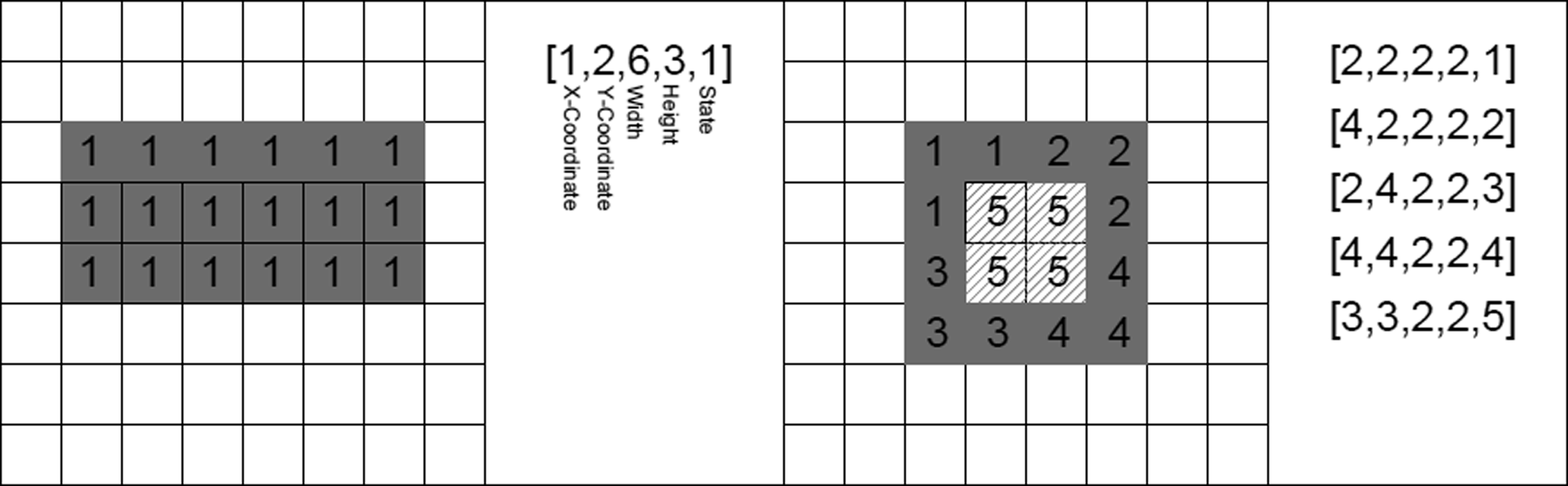
We now extend the GP-Systems first described by the author (2014). In this text, we describe the extension of mutators and evaluators and the performance of these new functions. The aim of the GP-System representation is to create a simple and easily re-creatable system for evolving floor plans discretised on a grid. As the system is designed for ED exploration, the evaluation and recombination stages (described in the previous section) are made extensible so that the users can add their own functions. A GP-System is composed of the following:

1. A 2D cellular array that holds a set of integer values. This can be seen as ‘space’ where the population member exists. All are initialised to have a state of ‘0’.

2. A genome which consists of a list of 5-tuples. When parsed into the cellular array, the five numbers are read as {1. X-coordinate, 2. Y-coordinate, 3. Width, 4 Height, 5. State}. So, reading the gene {1,4,6,7,3} would mean ‘go to the coordinate [1,4] and create a rectangle that is 6-cells wide, 7-cells high with a state of [3]'. The state can be coloured to make them easier to visualise. In the 2014 text, the genome was translated into a bit string, but in this work, it is kept as a set of integers to make designing the code for evaluators and mutators more interactive.

3. We will call a list of coordinates that represent a cluster (or connected) cells with the same state (or colour) as an ‘island’. While the simplest case is for a gene (t-tuple) to represent a single rectangle, two genes together with the same state can represent an ‘L’ or ‘T’ shape and a gene with a state of ‘0’ can represent a void by making a shape that is the same colour as the background.

The following table shows a two simple ‘floor plans’ and the corresponding genome, though there are multiple genomes that could have the same appearance.

A few algorithms are used to process the genotype (the 5-tuple list) into a phenotype (the cellular array and island set). These include the following:

1. A tracing algorithm that groups cells of similar state that are connected into ‘islands’.

2. The overall evolutionary algorithm which calls the subroutines to initialise, process, evaluate, select and rebuild the population.

3. In this implementation, using object-oriented programming, classes were used to encapsulate the ‘solution’, a niche, a GP-system, and Island and a Cell.

4. The mutators and evaluators are stored in lists within the solution class and each implements an abstract interface which describes how the algorithm will manipulate and read data off the functions.

5. Most of the visualisation is platform specific and uses proprietary frameworks. This research will only cover the algorithmic aspects of the implementation.

The algorithm begins with a description of the solution which consists of a set of room sizes and a list of connections as shown in the implementation written in the C# language.

public class GPSolution {

public List<IGPEvaluator> evaluators = new List<IGPEvaluator>();

public List<IGPMutator> mutators = new List<IGPMutator>();

private Dictionary<int, int > roomSizes = new Dictionary<int, int>();

private Dictionary<int, List<int>> roomConnections =

new Dictionary<int, List<int>>();

}

Below is an implementation for the recursive tracing algorithm:

public static void traceCell(int r, int c, int state, GPSystem gp,

Island island, int[,] statematrix)

{

if (gp.getMatrixValue(r,c) = = state)

{

statematrix[r, c] = 1;

island.addCoordinate(gp.getCell(r,c));

if (c + 1 < gp.numCol && statematrix[r, c + 1] ! = 1)

{

traceCell(r, c + 1, state, gp, island, statematrix);

}

if (r + 1 < gp.numRow && statematrix[r + 1, c] ! = 1)

{

traceCell(r + 1, c, state, gp, island, statematrix);

}

if (c - 1 > −1 && statematrix[r, c - 1] ! = 1)

{

traceCell(r, c - 1, state, gp, island, statematrix);

}

if (r - 1 > −1 && statematrix[r - 1, c] ! = 1)

{

traceCell(r - 1, c, state, gp, island, statematrix);

}

}}

Evaluators

The algorithm can take an arbitrary number of ‘evaluators’ each which implements the interface shown below. The only needed function is an evaluate function that takes in the GP-System and the solution description and outputs a floating-point number.

public interface IGPEvaluator

{

float evaluate(GPSystem gp, GPSolution gps);

}

Two of the most important criterions for a good plan are the correct room sizes and correct adjacencies. The algorithm for room sizes is quite straightforward – as each island is made unique, simply find the difference between the ideal island size and the actual size, so the perfect solution would have a fitness of 0 in this particular evaluator.

Evaluating adjacency

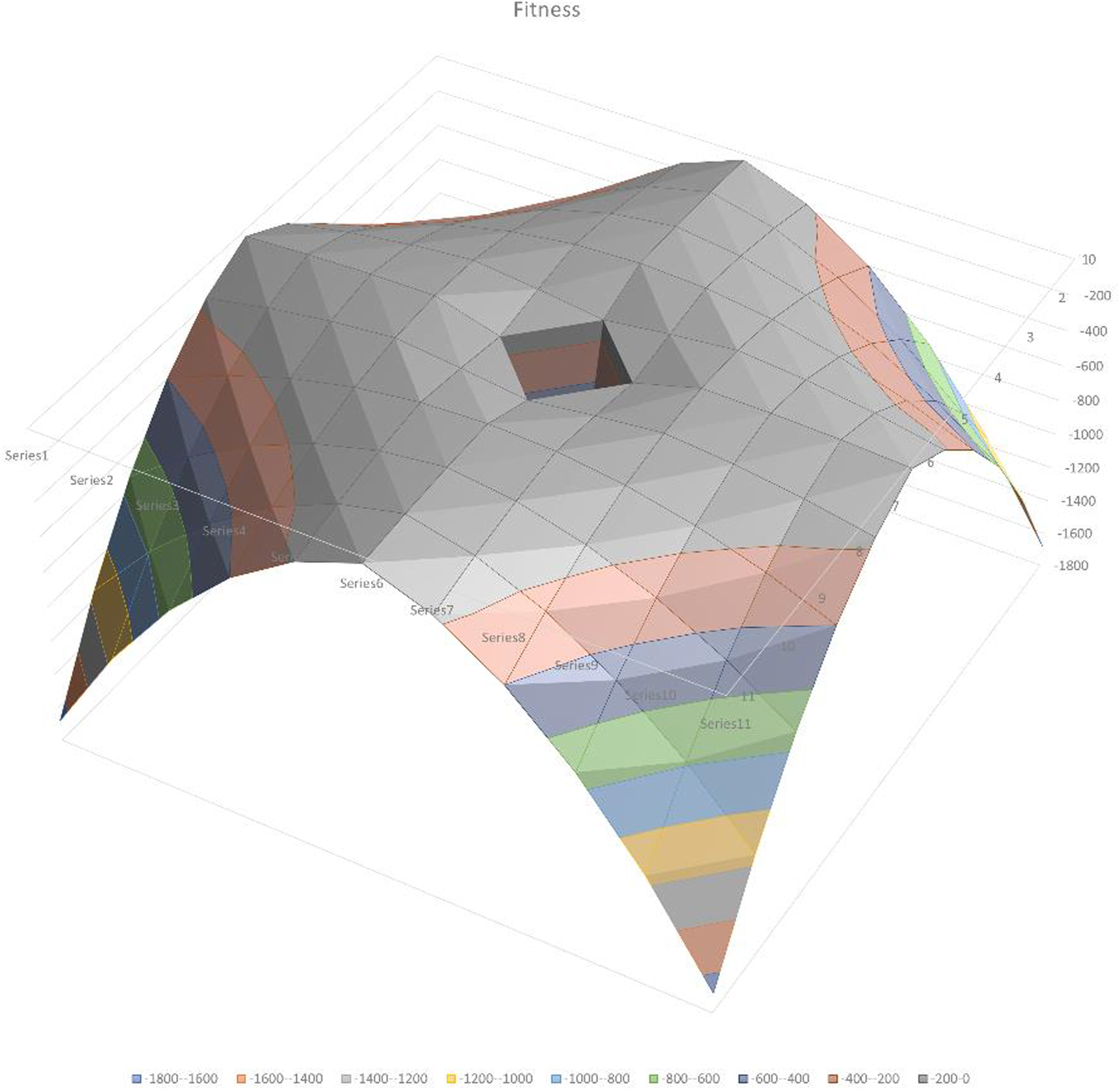
The most important factor to consider when designing evaluators for EC is to give as smooth as possible a gradient for the evolution to follow. The adjacency evaluator is a good example of how a problem that is binary (either the two islands are adjacent, or they are not) can be thought of in a way that works for evolution. The algorithm begins with finding the top-left most cell of the two islands and the bottom-right most cell. The rectangle bounds that bounds these two islands gives a total area, from which we subtract the areas of the two islands. Multiplying this by negative one gives the fitness. This way, the shorter the distance between the two, that is, the smaller the bounding rectangle, the higher the fitness.

However, this function cannot run in isolation as the two islands layered on top of each other gives an even better solution. A separate evaluator gives a big penalty for missing islands, so this scenario is avoided. Figure 4 shows the fitness landscape where Island ‘1’ is fixed and the x-coordinate and y-coordinate of Island ‘2’, are represented in the x- and y-axis of the space. In this example, the fitness was squared to smoothen out the fitness space. Note how they are four solutions, corresponding to Island ‘2’ being directly North, East, South and West of Island ‘1’.

Figure 4.

The calculations between the ‘adjacency evaluator’.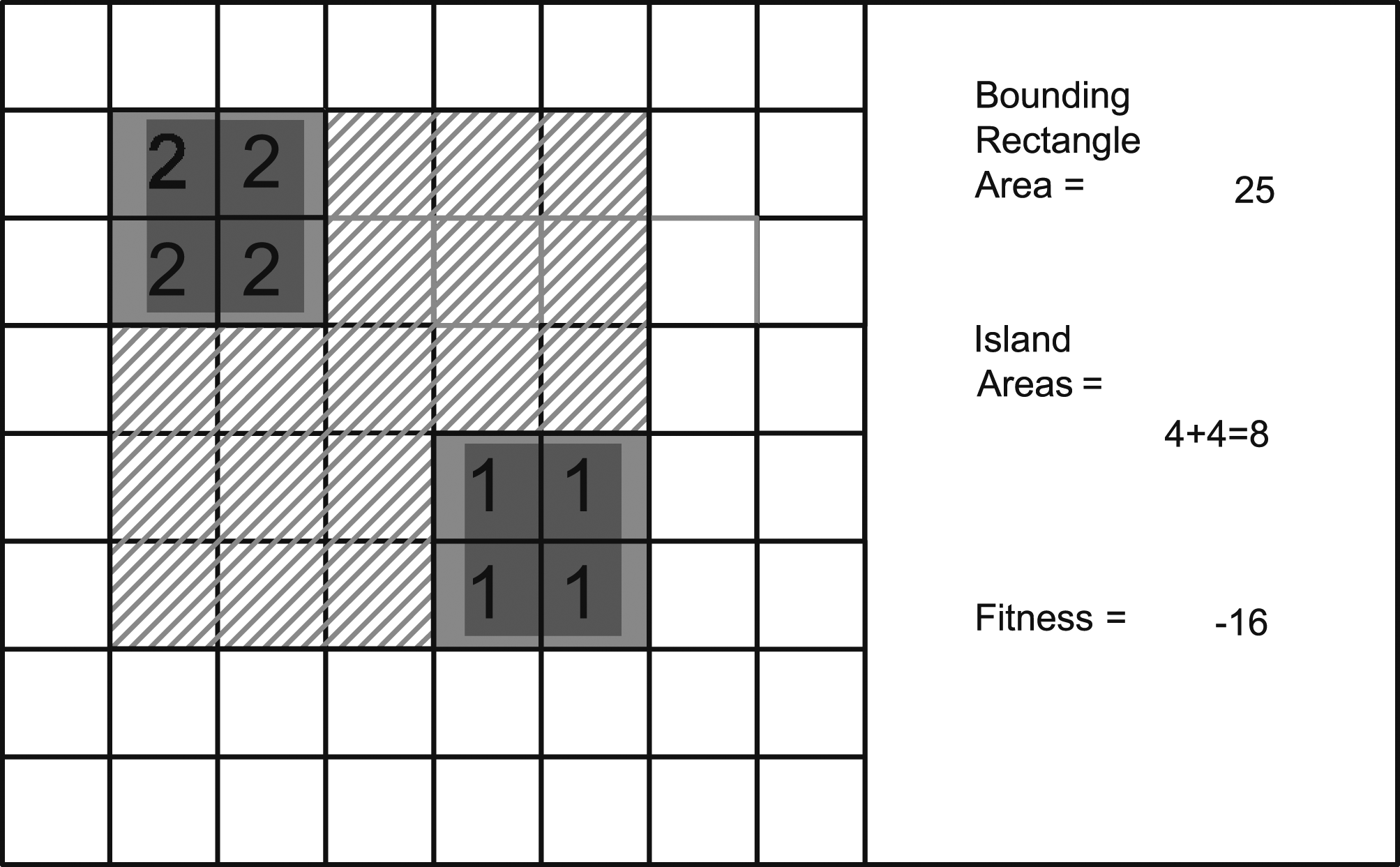

The dip in the middle occurs when the two Islands are in the same spot and the penalty for missing a room kicks in. The two room case is quite simple and converges very fast as would a hill-climbing approach or methods based on the gradient. The advantage of genetic algorithms is that with multiple rooms and instances where the evolution has to move to a lower fitness temporarily in order to have chance at the global maximum, the random mutations provide a mechanism by which this can happen.

public int evaluateAdjacency(Island A, Island B)

{

int ret = 0;

int minX = Math.Min(A.ULx, B.ULx);

int minY = Math.Min(A.ULy, B.ULy);

int maxX = Math.Max(A.LRx, B.LRx) + 1;

int maxY = Math.Max(A.LRy, B.LRy) + 1;

int totalAreal = (maxX - minX) * (maxY - minY);

int totalWidth = maxX - minX;

int totalHeight = maxY - minY;

if ((A.width + B.width = = totalWidth) &&

(A.height = = totalHeight ||B.height = = totalHeight))

{

return 0;

}

else if ((A.height + B.height = = totalHeight) &&

(A.width = = totalWidth ||B.width = = totalWidth))

{ return 0; }

return Math.Abs(totalAreal - (A.cells.Count + B.cells.Count));

}

The remailing core evaluators are described in Table 2.

Table 2.

Evaluators.

Evaluate edge cells	Gives a penalty for any Islands being outside of the grid. This reduces the number of plans considered as a line of mutation could lead to islands that are outside the grid, taking up processing time
EvaluateBoundaryCells	Try to reduce the perimeter of the floor plan by looking at the number of ‘0’ cells that are next to a coloured cell
EvaluateMissingRooms	A heavy penalty for missing rooms
EvaluateExcessRooms	A penalty is given for excess rooms, otherwise, the mutations that add more rooms would keep accumulating more rooms (even ones with zero area) without end
EvaluateRoomsSizes	Evaluate how close to the ideal room size each island is
EvaluateRoomsShapes	Give points for rooms that are not thin and narrow
EvaluateRoomConnections	Evaluate which rooms are connected to each other
EvaluateEfficiency	Give more points for an island being made of less genes, else an island that is made up multiple genes suffers from breaks where the fitness jumps very suddenly, for example, when they are no longer connected

Table 3.

Mutator list.

MutateDoNothing	Makes no changes – otherwise every solution is forced to mutate even after reaching an optimal state
MutateMoveLeft	Move the rectangle to the left
MutateMoveRight	Move the rectangle to the right
MutateMoveUp	Move the rectangle up
MutateMoveDown	Move the rectangle down
MutateMoveUpLeft	Move the rectangle diagonally to the upper-left
MutateMoveUpRight	Move the rectangle diagonally to the upper-right
MutateMoveDownLeft	Move the rectangle diagonally to the lower-left
MutateMoveDownRight	Move the rectangle diagonally to the lower-right
MutateGrowLeft	Grow the rectangle to the left
MutateGrowRight	Grow the rectangle to the right
MutateGrowUp	Grow the rectangle upwards
MutateGrowDown	Shrink the rectangle downwards
MutateShrinkLeft	Shrink the rectangle to the left
MutateShrinkRight	Shrink the rectangle to the right
MutateShrinkUp	Shrink the rectangle upwards
MutateShrinkDown	Shrink the rectangle downwards
MutateGrowLeftShortAndWide	Decrease the height and increase the width towards the left
MutateGrowRightShortAndWide	Decrease the height and increase the width towards the right
MutateGrowUpTallAndThin	Decrease the width and increase the height towards the top
MutateGrowDownTallAndThin	Decrease the width and increase the height to the bottom
MutateSwap	Swap the ‘state’ of two rectangles
MutateResize	Resize the rectangle to one of equal area if possible
MutateFlip	Flip the width and height
MutatePlaceLeft	Place the rectangle to the left of another randomly picked
MutatePlaceRight	Place the rectangle to the right of another randomly picked
MutatePlaceUp	Place the rectangle above another, randomly picked
MutatePlaceDown	Place the rectangle below another, randomly picked
MutateNewGene	Create a new gene with the next available state value

Table 4.

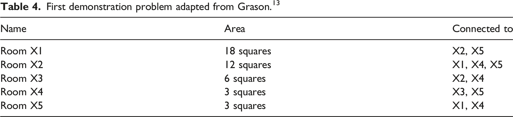
First demonstration problem adapted from Grason.¹³

Name	Area	Connected to
Room X1	18 squares	X2, X5
Room X2	12 squares	X1, X4, X5
Room X3	6 squares	X2, X4
Room X4	3 squares	X3, X5
Room X5	3 squares	X1, X4

Table 5.

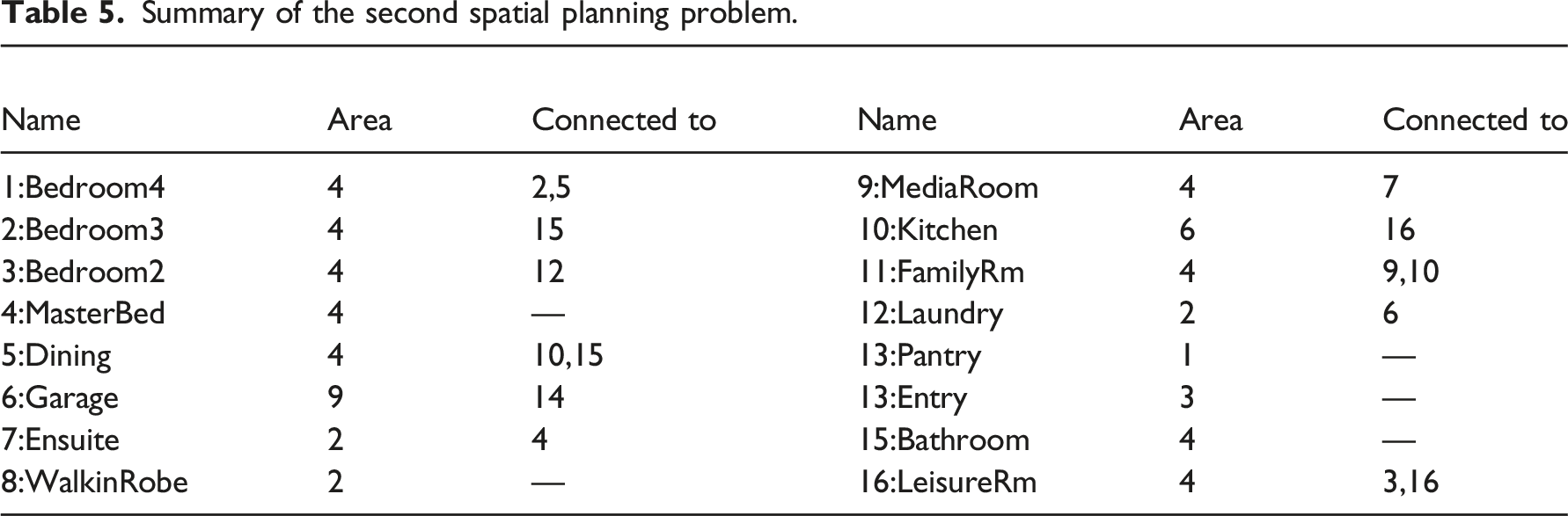
Summary of the second spatial planning problem.

Name	Area	Connected to	Name	Area	Connected to
1:Bedroom4	4	2,5	9:MediaRoom	4	7
2:Bedroom3	4	15	10:Kitchen	6	16
3:Bedroom2	4	12	11:FamilyRm	4	9,10
4:MasterBed	4	—	12:Laundry	2	6
5:Dining	4	10,15	13:Pantry	1	—
6:Garage	9	14	13:Entry	3	—
7:Ensuite	2	4	15:Bathroom	4	—
8:WalkinRobe	2	—	16:LeisureRm	4	3,16

Mutators

The Mutator class is structured in a similar manner to the Evaluator. The Mutator will implement a single function that alters the genes of a given GPSystem. A second argument determines the strength of the mutation (though many mutators do not make use of that) so that larger mutations occur less frequently, and smaller ones occur with higher frequency (Table 3).

public interface IGPMutator

{

void mutateGene(GPSystem gp, int index, int amount);

}

One possible way of designing the system was to operate directly on the genome, adding in a number to a random position on the array that represents each rectangle in the system. This would be similar to the bit-string crossover that is common in genetic algorithm literature. The problem here, is that some movements would be favoured over other, for example, having a rectangle grow to the left, would require two mutations – one to make the rectangle larger, and one to move its x-coordinate. On the other hand, growing to the right would only require one mutation (that of the width). So, to make sure that all four scenarios (growing up, down, left, right) occur with the same probability, it is better to design the mutation as a set of actions. This also allows for more complex mutations, for example, moving a rectangle, so that it is adjacent to another one, or moving an entire island.

A small tweak to improve the longevity of a line (trading off against a reduction in creating new forms), is to give a sixth value to each gene which represents ‘stability’. In other words, the algorithm can use this as a threshold before it allows that gene to be mutated. As an example, if the stability is set to three, and a random number between 1 and 10 is sought before the mutation is put forward, then there is a seven in 10 chance that the mutation will take place. If the value is nine, then there is only a one in 10 chance that it will change and with 10, the gene will continue to persist. This works in conjunction with a mutator that increases or decreases the stability of a gene. The danger of systems like this, is that it is much easier to get stuck circling around a local peak and having the niche filled with almost identical solutions. It becomes necessary to observe the meta-data of the niche and to have it clear out if it has been stagnating (while other niches have fitter solutions) without reaching the global maximum. Note that we rarely know what the global maximum is, with regard to all of the evaluators, only that we reached it with regard to the two core evaluators (the room sizes and connectivity) in which case both giving a fitness of ‘0’ means that those two core conditions have been met.

Demonstration

For the first example, the case given by Grason (Table 4)¹³ is used. Grason’s approach was to use graph theory, representing the connectivity as an embedded graph and then calculating the graph dual to get a rectangular floor plan. The research was noteworthy for the competition with which the entire algorithm was described as well as the achievement of having an implementation this early in the history of computer-aided design. The problem was described at the source in slightly different terms; room sizes (width and length) were set before hand, and the graph was complete, that is, every connection was named. By contrast, in the implementation described here, only the number of cells is given (a room of 12 squares could end up as 2 × 6, 3 × 4 or 12 × 1). Furthermore, a partial description of room adjacencies is allowed.

Table 5 summarises the spatial layout problem:

Running the problem for 200 generations without any heuristics specific to this problem or optimisations lead to an ideal solution relatively quickly. Though many more partial solutions (as shown on the right). (Figures 5 and 6)

Figure 5.

Running the problem through an evolutionary problem solver.

Figure 6.

Solutions to the second test problem.

As with many other problems, one of the most effective ways to reduce the size of the solution space is to fix one of the rooms so that it remains the same under initiation or mutation. For the second, problem, a modern residential floor plan was chosen arbitrarily, and its room sizes recorded (scaled so that the smallest space was one cell) as well as the connections particular to that plan. This is summarised in the table:

The problem took a lot longer to improve and was run for 2000 generations, although it was clearly visible that very little was changing in the upper echelon of solutions, because local high points had been reached and small changes were not helping. The most useful heuristic found in this case, was to increase the penalty in the boundary evaluator (shown on the right), which helped promote tighter plans in the early stages of the evolution.

A good strategy is to use a mix of algorithms, where a close solution is produced by the evolutionary system and in the last stage, a hill-climbing procedure is used. This saves on computation as with the larger problems the algorithm is more likely to find itself oscillating around a suboptimal peak.

Conclusion

In this research, a simple evolutionary scheme was demonstrated that can solve basic spatial planning problems. The advantages of evolutionary problem solving include the following:

1. Being able to take in an arbitrary number of heuristics.

2. Always proving a solution (even if it not the global optimum).

3. Providing an accessible was of utilising computational design (with the target audience in the fields of computer-aided design instead of computer science).

4. Not limiting the shapes of the floor plans design as opposed to many of the other approaches like graph duals or room placement.

Of greater importance to the field, is the use of evolutionary thinking, which such systems provide a path forward. The concepts introduced in evolutionary thinking include populational thinking, breaking down problems in terms of schema (looking for solutions are related, or part of the same lineage), as well as abstracting problems and their descriptions. It is clearly of benefit to the field that the performance aspect of design be formalised and the corresponding concept of fitness, forces users to think in these terms. The trade-offs in fitness are also an interesting aspect of any evolution and ED puts this as an important factor to consider by those designing the system.

In the experiments shown, most simply problems (less than six spaces) can be solved quick enough that they can be considered ‘real-time’ from a user-interactions. Larger problems are more interesting, as user interaction to guide the evolution leads to much more interesting results than letting the algorithm work autonomously. The experience thus far has been that ED can put forward solutions that are very close to optimised and that small nudge towards optimal final solution can be put forward by the human designer.

Indeed, user interaction is an aspect of ED that still needs more research and is worth pursuing as it is an interesting synthesis of human intuition with the brute force of computational calculation.

Footnotes

Declaration of conflicting interests

The author(s) declared no potential conflicts of interest with respect to the research, authorship, and/or publication of this article.

Funding

The author(s) received no financial support for the research, authorship, and/or publication of this article.

ORCID ID

Ruwan Fernando

References

Qian

Wang

. Advances in generative design. Comput Aided Des 2019; 116: 102733. DOI: 10.1016/j.cad.2019.102733

Delanda

. Deleuze and the use of the genetic algorithm in architecture. Archit Des 2002; 71(7): 9–12.

Bentley

. Evolutionary Design by Computers, San Fransisco, CA: Morgan Kaufmann, 1999.

Janssen

. Design Method and Computational Architecture for Generating and Evolving Building Designs. PhD Thesis. Hong Kong, China: Hong Kong Polytechnic University. 2004.

Sims

. Artificial evolution for computer graphics. In ACM SIGGRAPH’91 Proceedings. July 1991. San Diego, CA, USA. pp. 319–328.

Homayoumi

. A Survey of Computational Approaches to Space Layout Planning. 2006, https://citeseerx.ist.psu.edu/viewdoc/summary?doi=10.1.1.107.4372

Verma

Thakur

. Architectural space planning using genetic algorithms. In Proceedings of the 2010 The 2nd International Conference on Computer and Automation Engineering (ICCAE). February 2010. Singapore. pp 268–275.

Matthews

Craw

Elder

, et al. Applying genetic algorithms to multi-objective land use planning. In Proceedings of the 2000 Genetic and evolutionary computation conference (GECCO 2000): Joint Meeting of the 9th International Conference on Genetic Algorithms (ICGA-2000), and the 5th Annual Genetic Programming Conference (GP-2000). Morgan Kaufmann. pp. 613–620.

Keane

Brown

. The design of a satellite boom with enhanced vibration performance using genetic algorithm techniques. J Acoust Soc Am 1996; 99(4): 2599–2603.

10.

Van Laarhoven

Aarts

. Simulated annealing. In Simulated Annealing: Theory and Applications. 1987. Dordrecht, Netherland: Springer. pp. 7–15.

11.

Dutta

Sarthak

. Architectural space planning using evolutionary computing approaches: a review. Artif Intell Rev 2011; 36: 311–321. DOI: 10.1007/s10462-011-9217-y

12.

Jong

. Evolutionary computation. Wiley Interdiscip Rev Comput 2009; 1(1): 52–56.

13.

Grason

. An approach to computerized space planning using graph theory. In Proceedings of the 8th Design Automation Workshop. June 1971. Atlantic City, NJ, USA. pp. 170–178.

14.

Schnier

Gero

. Learning genetic representations as alternative to hand-coded shape grammars. In: Gero

Sudweeks

(eds) Artificial Intelligence in Design. Dordrecht, Netherland: Kluwer, 1996. pp 39–57.

15.

Damski

Gero

. An evolutionary approach to generating constraint based space-layout topologies. In: Junge

(ed) CAAD Futures. Dordrecht, Netherland: Kluwer Academic Publishing, 1997. pp 855–874.

16.

Gero

Kazakov

. Learning and re-using information in space layout planning problems using genetic engineering. Artif Intell Eng 1997; 11(3): 329–334.

17.

Rosenman

. The generation of form using an evolutionary approach. In: Dasgupta

(ed) Evolutionary Algorithms in Engineering Applications. Berlin, Germany: Springer, 1997. pp 69–86.

18.

Wong

SSY

Chan

KCC

. EvoArch: an evolutionary algorithm for architectural layout design. Comput Aided Des 2009; 41(9): 649–667.

19.

Caldas

. GENE_ARCH: an evolution-based generative design system for sustainable architecture. In: Smith

IFC

. (ed) Lecture notes in Artificial Intelligence. Berlin, Germany: Springer, 2006. pp 109–118.