Estimating the received solar irradiances by traditional vaulted roofs using optimized neural networks and transfer learning

Abstract

Traditional vaulted roof-forms have long been utilized in hot-desert climate for better indoor environmental quality. Unprecedently, this research investigates the possible contribution of machine learning to estimate the received solar irradiances by those roofs, based on simulation-derived training and testing datasets, where two algorithms were used to reduce their higher-dimensionality. Then, four models of ordinary least-squares and artificial neural networks were developed. Their ability to accurately estimate solar irradiances was confirmed, with R² of 95.599–98.794% and RMSE of 12.437–23.909 Wh/m². Transfer Learning was also applied to pass the stored knowledge of the best-performing model into another one for estimating the performance of new roof-forms. The results demonstrated that transferred models could provide better estimations with R² of 87.416–97.889% and RMSE of 79.300–13.971 Wh/m², compared to un-transferred models. Machine learning shall redefine the practice of building performance, providing architects with flexibility to rapidly make informed decisions during the early design stages.

Keywords

Solar irradiance prediction simulation machine learning transfer learning

Introduction

Traditional practices in architecture that integrate passive techniques presents itself as a sustainable and cost-effective solution for a better indoor environmental quality, especially in hot-desert climate.¹ Unlike active cooling systems, passive techniques, such as solar shading, passive cooling, and natural ventilation,² do not depend on mechanical acclimatizations. They seek controlling heat transfer through buildings to improve indoor environmental quality, and ultimately, reduce energy demand. Curved roof forms (CRFs), such as domes and vaults, are essential features of traditional architecture within hot climates of the Middle Eastern and North African region.³ Compared to flat roofs,^4–6 CRFs are attributed to many features on how they interact with the received solar irradiance, including partially exposed surface areas, thermal lag,⁷ and stack or chimney ventilation.^8,9

Research trendlines to estimate the performance of curved roofs

The landscape of scholarly literature that focused on studying the solar and thermal behavior of CRFs can be categorized into three lines of research that vary in the used technique and degree of sophistication. The first line entails early attempts^9–12 that present simple descriptions and guidelines for architects to consider, illustrating the capacity of CRFs to obtain lower indoor air temperature, due to less absorbed solar irradiance. Despite their significance, those attempts strongly call for further quantification studies, owing to the lack of supporting factual and empirical data.

Newly emerged techniques framed the second line of research that expanded previous abstracts into numerical and analytical methods. Among them is the early work of Pearlmutter,¹³ who quantitatively compared solar exposure and thermal behavior of vaulted roof forms (VRFs) against flat roofs, obtained from mathematical and physical models. Few papers followed this attempt to study the performance of CRFs. Elseragy¹⁴ established the theoretical idea of “self-shading,” based on mathematical models that determine the received solar irradiance on CRFs of various configurations to validate their thermal benefits. Gómez-Muñoz et al.¹⁵ studied the performance of VRFs by numerical methods, portraying the notion of “auto shading” as a valuable property of such forms. This attribute were also endorsed by Hadavand and Yaghoubi¹⁶ and Hadavand et al.¹⁷ who used several energy and solar irradiance mathematical models to compare heat transfer patterns of CRFs against flat roofs, in terms of solar irradiances and wind-flows. Tang, et al.¹⁸ examined the absorbed solar irradiance by CRFs, compared to flat roofs. In follow-up studies,^7,19 they proposed a finite element model to analyze the thermal performance of CRFs, based on heat transfer equations, verifying the capability of CRFs to provide less indoor temperatures, compared to flat roofs. Faghih and Bahadori^20,21 also utilized numerical methods to estimate the solar irradiance and thermal performance of domed roof forms (DRFs), under various weather conditions. While useful, these studies did not bring much attention to architects, who lack the required skills to perform such numerical methods. This is evident in the scarcity of published studies of that domain.

Supported by the progress of multicore computer processors^22,23 that drove the emergence of many simulation tools,²⁴ the third line of research, known as white-box, entails new approach that integrates simulation²⁵ with parametric investigations to generate and test plentiful design scenarios. Ayoub and Elseragy⁴ employed the parametric ability of Grasshopper²⁶ to generate 248 DRFs. The received solar irradiances by such roofs were compared to flat roofs by Autodesk Ecotect. They showed that DRFs could reduce both the intensity of the received solar irradiance and the required cooling energy in hot-desert climates. Elnokaly et al.⁵ presented the first attempt to study the performance of VRFs via machine learning algorithms (MLAs). 2310 VRFs were generated, where Diva-for-Grasshopper²⁷ was used to simulate their solar and thermal behavior. With 11 variables, Principal Component Analysis (PCA) was used to extract hidden information. This revealed interesting correlations among variables, realizing solar and energy performance of VRFs geometries. Recently, Ayoub²⁸ compared single- and ensemble-models to estimate the solar irradiances and energy consumption for VRFs with various configurations.

This accurate engineering approach is only half the story, while the accompanying challenges building design community is facing the other half; and they are arguably as important as the estimations themselves. Solar irradiance simulations require complex input data, including weather file,^29–31 sky model,^32,33 space geometry, and nearby contexts.³⁴ Even with today’s computers, these simulations are inherently time-consuming and require expensive computations³⁵ to investigate the performance of multiple design scenarios. Although previous efforts have put the focus to integrate simulation techniques into design process,³⁵ many of the existing tools exhibit a degree of impracticality that might disrupt the flow of design process,²⁴ especially during the early conceptual stages.³⁶

Machine learning approach

The field of building performance estimations has been witnessing incremental advances in predictive models that build on MLAs, known as black-box. They entail learning from relevant data to discover hidden patterns, based on mathematically fit models, without being directed to perform such tasks.³⁷ Machine learning algorithms can achieve accuracies that are close to training simulation data, yet with less computations. The literature includes several attempts that employed MLAs to predict daylighting,^38–41 sky models,^42–46 weather elements,^47–50 artificial lighting,^51,52 and solar radiation.^53–55 However, using MLAs to predict the performance of VRFs is still underexplored. Apart from Ref. 28, to the author’s best knowledge, hardly any research could be found in literature that sought to predict the received solar irradiance on CRFs via MLAs. Such scarcity can be attributed to the relatively novel, yet promising, field of application.

Research aim

This research is a continuation of an ongoing study that explores the reciprocal relationship between the received solar energy by curved roofs and their different geometrical configurations, building upon the simulation results of a previously conducted study by the author.⁵ This research tackles previous limitations by replacing the sophisticated simulations with MLAs to predict the performance of VRFs of various configurations. It unprecedently seeks to assess the potential contribution of regression MLAs to acquire preliminary approximations on the received solar irradiance of VRFs. It is worth mentioning that this research addresses a distinct aspect of solar irradiance estimation, specifically filling the gap in existing literature on estimating the performance of traditional vaulted roofs, which is a novel aspect not extensively explored in the existing literature. While prior attempts have addressed solar irradiance prediction using machine learning,^56,57 they mostly concentrated on general solar exposure estimation. This research is structured as following: The Methodology section highlights the proposed methodology, the Results and Discussion section summarizes and discussions the solar simulation and MLAs results, followed by the Conclusion section that presents overall conclusions of the research.

Methodology

The methodological procedure is realized through a 3-phase process (Figure 1). The received average hourly direct normal irradiance (AHR_Direct) and diffuse horizontal irradiance (AHR_Diffuse) (Wh/m²) on VRFs are calculated via (i) Solar Irradiance Simulations, providing training and testing datasets for regression models. A parametric algorithm in Grasshopper is developed to derive the modeling and simulation of VRFs, consistent with (i-i) Geographical Location and Temporal Settings, (i-ii) Internal and External Variables, and (i-iii) Simulation Tool and Parameters. Different scales and magnitudes of independent variables of simulation datasets are brought into common scale before conducting further analysis in (ii) Dimensionality Reduction via (ii-i) Data Re-Structure. (ii-ii) Horizontal and (ii-iii) Vertical Reduction of data are then utilized to improve the prediction accuracy of regression models by keeping important variables, while removing less significant ones. The reduced datasets can then be used to conduct (iii) Regression Analysis via (iii-i) Ordinary Least-Squares Regression (OLS) and (iii-ii) Artificial Neural Networks (ANNs). The hyperparameters of ANNs are optimized in (iii-iii) Hyperparameters Optimization, where the resulting models are compared against their prediction accuracy in (iii-iv) Performance Evaluation. Lastly, the stored knowledge in these models is passed into new ones using (iii-v) Transfer Learning (TL) to predict the performance of additional roof forms.

Figure 1.

Research methodological procedure, showing the used applications and MLAs and the sequence of data processing.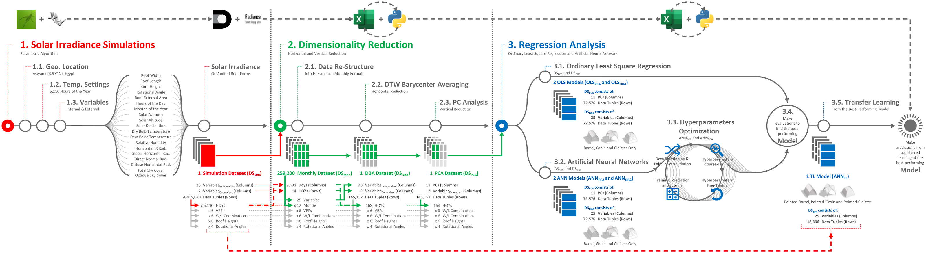

Solar irradiance simulations

Study geographical location and temporal settings

Aswan (23.97° N), Egypt, is selected as the study location, situated in Hot-Desert climate zone.^58–60 Its EnergyPlus Weather (EPW) file is representative of weather dataset from the Egyptian Typical Meteorological Year.⁶¹ The annual trends of Direct Normal Radiation (DNR) and Diffuse Horizontal Radiation (DHR) extracted from EPW file are explored. They are converted into Monthly Average Hourly Direct Normal (DNR_Monthly) and Diffuse Horizontal Radiation (DHR_Monthly), respectively. Both address all observations of the first hour of each day in a given month to calculate the monthly average hourly solar irradiance. Then, they take all observations of the second hour of each day in the same month to calculate their average, repeating this procedure for all months. (Figure 2) plots DNR_Monthly and DHR_Monthly on y-axis against hours of the day on x-axis. It shows higher values of direct component, compared to diffuse component, due to the prevailing clear sky. The simulations are conducted on annual basis, considering a fixed range diurnal hours (5:00–18:00) to avoid unnecessary calculations, where the impact of solar radiation is undetected.⁶² This yields 5110 (14 Hours × 365 Days) Hours of the Year (HOYs) for that specific location.

Figure 2.

Average hourly values of direct normal (left) and diffuse horizontal (right) radiations (Wh/m²) for Aswan.

Internal and external variables

Architecturally, VRFs come in variety of geometries (Figure 3),⁵ ranging from Barrel Vaults that resemble continuous semicircular arch, to Groin Vaults that consist of two intersecting barrel vaults crossing each other, to Cloister Vaults that contain four concave arched surfaces, meeting at a center. In addition, the investigations will consider pointed variations to those roof forms.

Figure 3.

Examples of the investigated vaulted roof forms.⁵

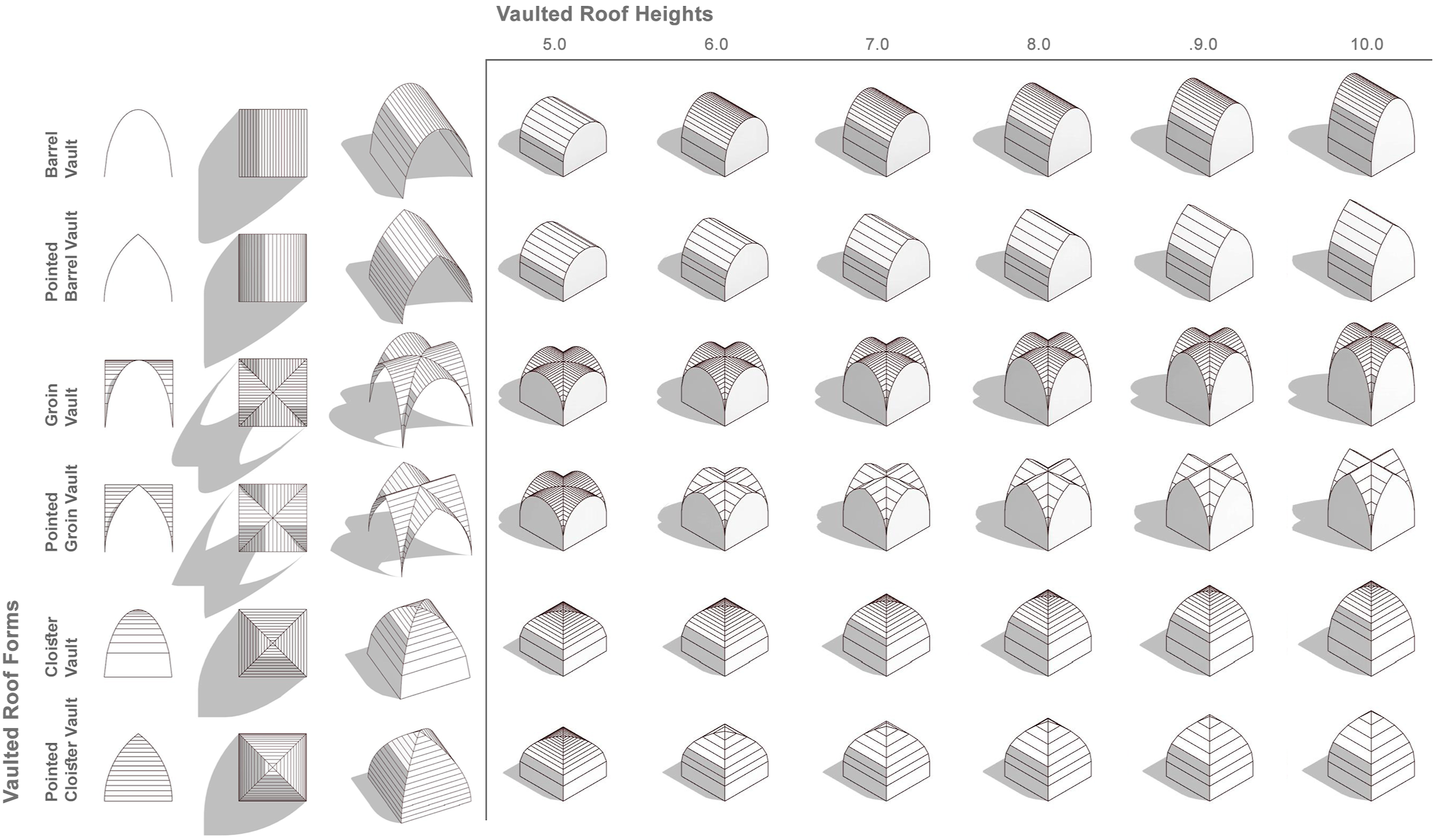
Previous studies have demonstrated that the solar performance of VRFs is affected by several internal variables, including geometries and orientations,^5,63,64 in addition to other external variables related to weather elements.^35,65 The internal variables are represented by different ranges of geometrical configurations (Figure 3), including width, length, height, and rotational angle. Both width and length have three incremental steps (5.00, 7.50 and 10.00), yielding 6 width/length combinations (10.0 × 7.5, 10.0 × 5.0, 7.5 × 5.0, 7.5 × 10.0, 5.0 × 10.0 and 5.0 × 7.5), whereas the height has six incremental steps (from 5.00 to 10.00). Rotational angle has only four incremental steps (0.00°, 45.00°, 90.00°, and 135.00°), as VRF at 0° is identical to 180°. This yields 864 VRFs (6 roof types × 6 width/length combinations x six roof heights × four rotational angles).

The Majority of external variables are obtained from EPW file.^66,67 Some weather elements do not either exhibit variability or contribute to the received solar irradiances, which include atmospheric pressure, external illuminance, wind direction and speed, visibility, ceiling height, and precipitation Thus, they are not considered in the analysis. Other set of external variables has been examined in previous studies to predict the received solar irradiance,^68,69 such as temporal data, Solar Azimuth (SAzi), Solar Altitude (SAlt), and Solar Declination (SD) (Figure 1). Temporal variables are represented by Hours and Months, as a series of 5110 timesteps. SAzi and SAlt are obtained by inputting the weather data file into Sun Path, a Diva-for-Grasshopper²⁷ component. SD is calculated from equation (1),⁷⁰ which is adjusted for hourly resolution

{S D}_{H o u r l y} = 23.45 \times \sin (360 ° \frac{(284 + ((H O Y + 1) / 24))}{365} \times \frac{π}{180})

(1)

Simulation tool and parameters

Grasshopper 3D is used to develop a parametric algorithm to derive the modeling of VRFs, building upon geometrical transformations. The variables of VRFs are first input, where the algorithm generates various VRFs geometrical configurations. Those models are sent to Diva-for-Grasshopper to perform solar irradiance simulations. As a plug-in that operates under Grasshopper, Diva-for-Grasshopper interfaces the validated Radiance engine²⁵ for daylight and solar analysis. The input simulation parameters are accuracy: 0.10, bounce: 4, division: 1024, resolution: 256, and sampling: 256. Each model is discretized into smaller parts with grid spacing of 0.45 m.

Dimensionality reduction

Data re-structure

Standardization is used to bring the entire data to a common scale, preventing variables of larger values from dominating the learning. Randomization is also utilized to randomly shuffle all data rows to prevent their order from affecting the learning. Still, models constructed from pre-processed data may introduce some limitations related to the increased number of variables and datapoints. While depending on many variables can improve accuracy, this comes at the expense of interpretability. Inversely, fewer variables can ensure interpretability, but can increase the risk of overfitting.³⁵ Thus, the high-dimensionality of data are vertically reduced to find essential variables for developing models. Again, reduced variables with plenty datapoints require memory-intensive calculations that take extended periods of time, making the process less efficient. The embedded temporal dimensions are exploited to horizontally reduce the data, converting them into sets of continuous time-series, each includes a sequence of datapoints.

Horizontal reduction: Dynamic time warping using barycenter averaging

This step entails acquiring averaged representative time-series that maintain the temporal attributes and reflect similarities of the original data with less datapoints. First, important frequencies are extracted using periodogram analysis,⁷¹ explaining the embedded periodic pattern. Representative time-series can be obtained via K-means or Agglomerative Hierarchical Clustering that average a set of sequences according to point-to-point Euclidean distance measure among datapoints.⁷² Dynamic Time Warping (DTW)⁷³ (Figure 4) replaces point-to-point distance with many-to-point alignment.⁷⁴ For two time-series of lengths (n) and (m), respectively, DTW creates a matrix that consists of (n × m) elements. Each element (e_i,j) represents possible squared distances (d_i,j) between (t_j) and (s_i), plus the minimum of three surrounding neighbors at positions: (i − 1, j − 1), (i − 1, j), and (i, j − 1). The optimal warping path can then be built by tracking the minimum of three surrounding neighbors across the entire matrix.

Figure 4.

The obtained warping path of two paired time-series, showing the difference between the distance alignments of (a) Euclidean point-to-point and (b) DTW many-to-point.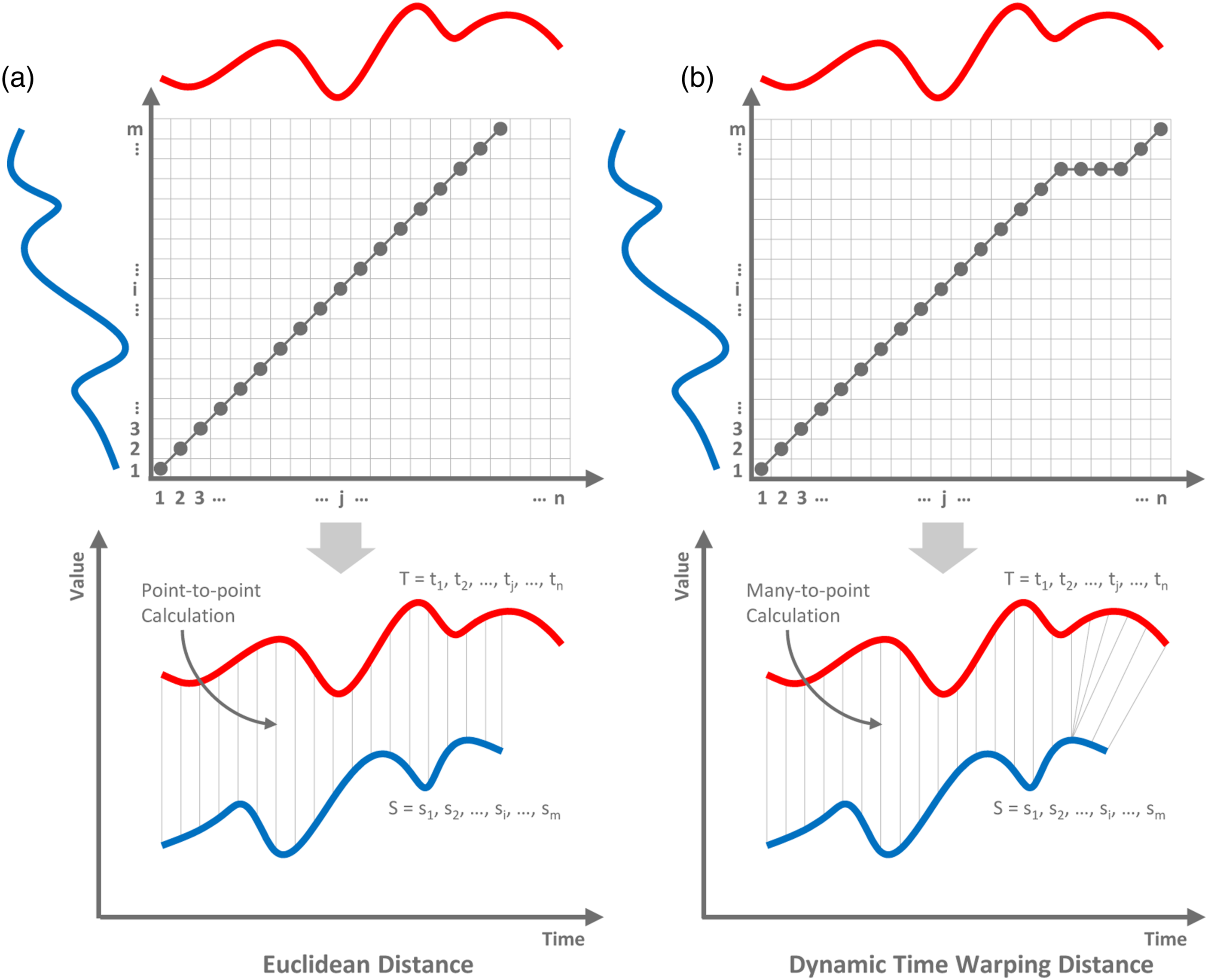

While DTW can only be used to average two time-series, Petitjean et al.⁷⁵ introduced DTW Barycenter Averaging (DBA) to find averaged time-series from several sequences. DTW Barycenter Averaging randomly selects an averaged time-series, where a set of DTWs is calculated between the temporary time-series and every original time-series to find initial associations between their datapoints. Each datapoint in the temporary time-series is reassigned as the barycenter of datapoints associated to it. New DTWs are recalculated between the updated averaged time-series and every original time-series, updating the associations between their datapoints. This process continuous iteratively until the averaged time-series is obtained. DBA is conducted in Python using a modified code from DBA.py.⁷⁶

Vertical reduction: Principal component analysis

The second step aims at reducing high-dimensional data vertically via PCA.⁷⁷ Principal component analysis merges the original data into a set of uncorrelated Principal Components (PCs), defined as pairs of “eigenvectors” that imply the spread directions of the new feature space, and “eigenvalues” that denote the magnitudes of that spread.⁷⁸ Dimensionality reduction is achieved by considering significant PCs that hold the highest variance of the original data. Applying PCA on time-series should reflect the original temporal order of datapoints.⁷⁹ Eigenvalues and cumulative variances of all PCs are arranged to find the first few that explain over 95% of the original variance^78,80,81 without losing critical information,⁸² while disregarding less important PCs. Principal components that have eigenvalues above 1.00 are deemed significant, and will be exploited in regression analysis. Factor loadings can reveal the correlation between the original variables and respective PCs. Variables of larger factor loadings are well represented by their PCs, and vice versa.

Regression analysis

Ordinary least-squares regression

Ordinary least-squares regression is a method of performing numerical predictions⁸³ via a linear equation that fits the dataset, where a dependent variable ( $y_{i})$ varies according to the input independent variables ( $x_{i}$ ). OLS seeks to minimize the sum of squared errors (SSE) between the observations and predictions. Since there is no hyperparameters for OLS, the hyperparameters optimization will only consider optimizing ANN.

Artificial neural networks

ANN is a non-linear algorithm that performs numerical predictions via supervised learning techniques. It consists of an input layer, one or more hidden layers, and an output layer that produces predictions. Neurons within each layer are connected to those in the next layer with assigned weights.⁸⁴ During training, inputs are multiplied by their respective weights and modified by bias,^85,86 then passed through an activation function to determine whether the data is transmitted to the next layer. This process is repeated across the network until reaching the output layer, which produces the final prediction. The weights are tuned during training to minimize prediction errors, using a backpropagation procedure that iteratively updates the weights until a termination criterion is met.⁸⁷ Artificial neural networks were chosen in this research due to their ability to handle complex relationships and capture non-linear patterns in the solar irradiance prediction task. While transfer learning, as will be clarified in the Transfer Learning section, can typically be applied in pre-trained ANN models, is not directly applicable to other MLAs, such as Support Vector Regression (SVR). The training, calculation, evaluation, and optimization of all MLAs are carried out in Python using scikit-learn library.⁸⁸

Hyperparameters optimization

The pre-processed data is split into two parts, the largest is used for training, while the smallest is held back for testing the performance against predictions made by the model. To avoid statistically unbalanced training and testing data in Artificial Neural Networks (ANNs), K-Fold cross-validation is used. The pre-processed data is split into a training set and a smaller testing set. K-Fold cross-validation splits the training set into K smaller folds, with (K-1/K) of the data used for training and (1/K) used for validation. The model is trained iteratively on (K − 1) folds for K times, while the remaining (K^th) fold is used for validation. This approach helps to improve the reliability and generalization performance of the model, while avoiding overfitting. To optimize the performance of ANNs, various techniques have been developed to identify the optimal combinations of hyperparameters.^89–91 Yet, such approaches can be impractical in actual applications,⁹² thus, coarse- and fine-tuning methods are used instead. Grid search is used in coarse-tuning to test wider bounds of hyperparameters and identify high-bias areas that indicate underfitting training data, while high-variance areas signify overfitting but fail to accurately predict validation data. Fine-tuning relies on Bayesian Optimization (BO)⁹³ to uncover the optimal combinations of hyperparameters with less iterations. It involves Bayesian surrogate model to estimate the objective function, and acquisition function to optimize the selection of hyperparameters at each iteration.^94,95 BO iteratively estimates the behavior of the objective function and selects candidate hyperparameters until the maximum number of iterations is reached. Scikit-optimize⁹⁶ is used to perform BO, as it is well-integrated with scikit-learn library. The developed ANN model with fine-tuned hyperparameters is instructed to stop training if the errors remain unchanged for a given number of iterations to prevent overfitting.

Evaluation metrics

Root Mean Square Error (RMSE) (2) is used in this research, as it converts the squared errors into their original units, making them easier to interpret. While there is no correct value range for RMSE, its significance lies in differentiating the accuracy of regression models. R² (3) is also employed to report the ratio between the total explained variance by a model and the total variance of observed data

R M S E = \sqrt{\frac{1}{n} \sum_{i = 1}^{n} {({\hat{y}}_{i} - y_{i})}^{2}}

(2)

R^{2} = 1 - \frac{\sum_{i = 1}^{n} {({\hat{y}}_{i} - y_{i})}^{2}}{\sum_{i = 1}^{n} {(y_{i} - {\bar{y}}_{i})}^{2}}

(3)

where

({\hat{y}}_{i}

) is the predicted value at timestep (

i)

, (

y_{i})

is the observed/simulated value at timestep

(i)

, (

{\bar{y}}_{i})

is the average value, and (

n

is the number of datapoints that are used for evaluation.

Transfer learning

After training and validation, ANN model is utilized to predict new VRFs. Since it is not trained to predict such new problems, it is expected to yield inaccurate results. Obtaining new training data via simulations to build a new model would require further computations. Thus, TL⁹⁷ is utilized to transfer the stored knowledge from a pre-trained model into a new model. This requires far less training data than to train a new model, significantly improving the computational efficiency. TL begins by extracting the developed ANN model, where the hidden layer that was trained previously is frozen and becomes untrainable. The output layer is replaced with a new one to present new predictions. With this new model, only the last layer is trained, with the same hyperparameters, using a fraction of the original training data. Currently, scikit-learn does not natively support TL. Thus, another model is created by keras⁹⁸ on which TL is performed that is equivalent to the best-performing model, obtained from scikit-learn.

Results and discussion

Solar irradiance simulations

The annual simulations of solar irradiance were performed on VRFs, yielding 864 datasets (6 VRFs x 6 width/length combinations x six roof heights x four rotational angles), each consisted of 21 columns (19 independent +2 dependent variables) and 5110 rows (HOYs). 4 additional columns were added to that data, acting as numerical identifiers of six VRFs categories using One-hot encoding.⁹⁹ The first three columns signify the categorical VRFs variables of Barrel, Groin, and Cloister, while the last column represents Curved/Pointed VRFs. Each column has inputs of 0 for all categories, except for a specific category that has an input of 1. This way, the combined Simulation Dataset (DS_Sim) includes 25 columns (4 identifying variables + 19 independent + 2 dependent variables) and 4,415,040 rows (864 datasets × 5110 HOYs).

For illustrative purposes, AHR_Direct and AHR_Diffuse of only Barrel VRF results from DS_Sim are plotted in (Figure 5) due to space limitations. It grouped the results into two horizontal sections: the first showed curved Barrel, while the other was for pointed variation. Each section was divided into six vertical parts, signifying one of the pre-defined 6 width/length combinations. Each horizontal section included eight horizontal parts, representing four rotational angles with only two roof heights. Following the idea explained in the Study Geographical Location and Temporal Settings section, solar irradiance results of AHR_Direct and AHR_Diffuse were encapsulated into Monthly Average Hourly Direct Normal Irradiance (MAHR_Direct) and Monthly Average Hourly Diffuse Horizontal Irradiance (MAHR_Diffuse). (Figure 5) shows MAHR_Direct on primary y-axis and MAHR_Diffuse on secondary y-axis, against diurnal hours of the day (5:00–18:00) on x-axis.

Figure 5.

Examples of (a) Barrel and (b) Pointed Barrel VRFs, showing their MAHR_Direct and MAHR_Diffuse from DS_Sim.

Dimensionality reduction

Data re-structure

Preliminary inspections of the resulting DS_Sim revealed an insignificant amount of missing AHR_Direct and AHR_Diffuse values, constituting less than 1.6% of total datapoints. To keep DS_Sim consistent, missing datapoints were replaced by mean values from their immediate neighboring values. This way, DS_Sim was ready to be represented as sequences of continuous time-series of varying periods and amplitudes. In Microsoft Excel, the original data domain was transformed into frequency domain using Fourier analysis,¹⁰⁰ where periodogram analysis was then conducted. Data frequencies were plotted on x-axis against their amplitudes on y-axis (Figure 6). This revealed large amplitude of frequencies at 0.041768 Hz, equivalent to 23.942 ≈ 24 h, and 0.083393 Hz, corresponding to 11.991≈12 h. The first frequency was selected as dominant behavior, because it agrees with the overall trend of MAHR_Direct and MAHR_Diffuse, confirmed by repeating curves on daily basis, as shown in (Figure 5).

Figure 6.

Periodogram analysis of randomly selected 24 examples from DS_Sim.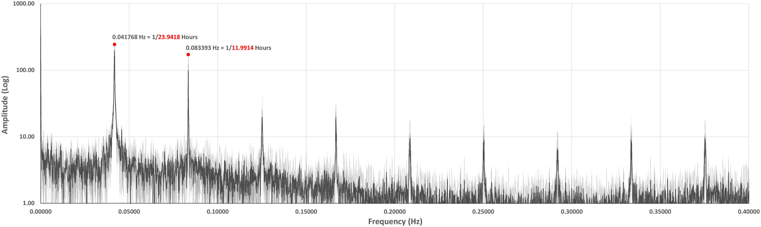

To convert the structure of DS_Sim into suitable format for DBA. py, it was hierarchically re-structured into smaller sets of time-series, following the established dominant behavior. Each represented a single variable (column) with 5110 rows (HOYs). Every column was then partitioned chronologically into 12 datasets, resembling months of the year, each consisted of 434 datapoints for January (14 h × 31 days), 392 datapoints for February (14 h × 28 days), etc. The resulting 259,200 Monthly Datasets (DS_Mon) (6 VRFs × 6 width/length combinations × six roof heights × four rotational angles × 25 variables × 12 months) were re-arranged into tabular format, each consisted of 28–31 columns (according to the number of days of months) and 14 rows (diurnal hours). This way, the first row of every DS_Mon included datapoints of the first diurnal hour of each day in a given month, whereas the second row represented datapoints of the second diurnal hour of each day in that month, and so on.

Horizontal reduction: Dynamic time warping using barycenter averaging

The re-structured 259,200 DS_Mon acted as sets of time-series that were fed one-by-one into DBA.py to be horizontally reduced. The averaged set of time-series were created by aligning each individual time-series with a temporary average one. The optimal alignment could be obtained by DTW that iteratively compute and update the temporary barycenter until the average of each time-series was acquired. The results were combined into DBA Datasets (DS_DBA), which included 25 columns (4 identifying variables + 19 independent variables + 2 dependent variables) and 145,152 rows (864 datasets x 14 diurnal hours × 12 months). This way, the original DS_Sim could horizontally be reduced from 4,415,040 to 145,152 rows. To clarify, AHR_Direct and AHR_Diffuse from DS_DBA, with their relative ranges from DS_Mon data, were plotted only for Barrel VRF (Figure 7). The figure grouped the results into two horizontal sections: the first showed curved Barrel, while the other was for pointed variation. Both sections were divided into six vertical parts, each representing one of the pre-defined 6 width/length combinations for March and September. Each horizontal section included eight horizontal parts, signifying four rotational angles with two roof heights. The charts plotted AHR_Direct on the primary y-axis and AHR_Diffuse on the secondary y-axis against diurnal hours of the day on x-axis.

Figure 7.

DBA outputs from DS_DBA and ranges of their equivalent results from DS_Mon of (a) Barrel and (b) Pointed Barrel VRFs, showing their AHR_Direct and AHR_Diffuse for March and September.

Vertical reduction: Principal component analysis

The input data from DS_DBA, including 23 columns and 145,152 rows, without dependent variables, was vertically reduced by PCA. This analysis does not require randomization, though the used dataset was standardized before dimensionality reduction. In scikit-learn, data standardization was conducted via Standard Scaler, which scales and centers the transformed data such that its mean becomes 0.00, which is essential for PCA. (Figure 8(a)) shows the developed eigenvalues and cumulative variances of the resulting 23 PCs in a descending order of magnitude. The first 13 PCs represented 97.12% of the cumulative variance of DS_DBA. This representation decreased drastically in latter PCs, where the remaining 10 PCs explained only 2.88% of DS_DBA. Again, (Figure 8(a)) confirms that, of all the developed 13 PCs, the first 11 PCs are having eigenvalues more than 1.00, explaining 92.28% of DS_DBA. Thus, they were considered significant, and shall be exploited in the following regression. Inversely, the other 12 PCs explained only 7.73% of the original DS_DBA. Thus, they were deemed less significant, and could be disregarded, without affecting the quality of data. This way, the independent variables of the original DS_DBA could be vertically reduced from 23 to only 11 dimensions. PCA yielded vertically reduced PCA Dataset (DS_PCA), which included 13 columns (11 PCs as independent variables + 2 dependent variables) and 145,152 rows.

Figure 8.

Summary of PCA analysis for all VRFs, showing (a) eigenvalues and cumulative variances of the developed PCs, in addition to (b) factor loadings between the original variables and the developed PCs.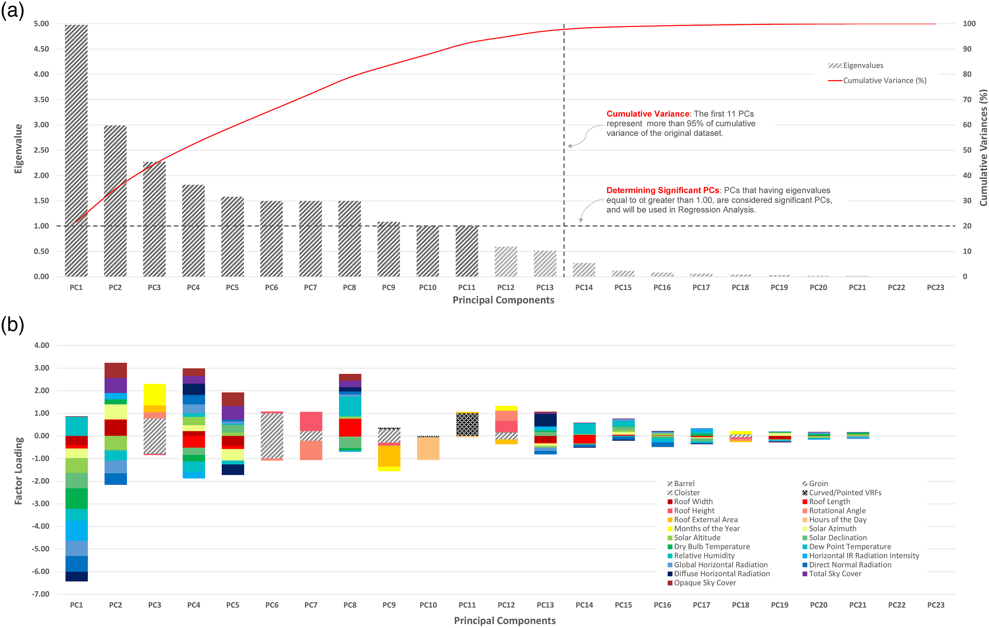

The impact of significant PCs on the whole data can be realized by plotting their factor loadings, which define the correlations between the original variables and their corresponding PCs (Figure 8(b)). Such correlations can be interpreted not only from a statistical perspective, but also from an architectural point of view. The figure revealed that PC1 is strongly correlated with SAzi, SAlt, SD, DBT, DPT, RH, HIrR, GHR, DNR, and DHR (representing Solar Radiation). PC2 is strongly correlated with SAzi, SAlt, GHR, DNR, TSC, and OSC (representing Diurnal Daily Motion). Collectively, PC4, PC7, PC8, and PC9 are highly correlated with Roof width, Roof Length, Roof Height, Rotational Angle, and Roof External Area, making them representatives of Roof Configurations. PC5 is highly correlated with SAzi, TSC, and OSC (representing Sky Cloudiness). PC3 and PC6 are highly correlated with Barrel, Groin, and Cloister categories, making them representatives of VRF Types. PC10 is strongly correlated with Hours of the Day (representing Temporal Settings). Lastly, PC11 is highly correlated with Curved/Pointed VRFs (representing Roof Curvature. It can be concluded that Solar Radiation–related variables, especially GHR, DNR, and HIrR were well represented by the first 2 PCs. Other related variables, such as SAzi, SAlt, SD, DBT, DPT, and RH were also tolerably represented by such PCs. These variables are imperative to characterize the received solar irradiances by VRFs. The contribution of internal variables by the first 2 PCs, including Roof width, Roof Length, Roof Height, Roof External Area, and Months of the Year, were relatively less significant, but were represented dispersedly by other PCs. This is expected, since their variations in DS_DBA do not change on regular basis, compared to Solar Radiation–related variables that fluctuate rapidly on daily and monthly basis.

Regression analysis

Ordinary least-squares regression

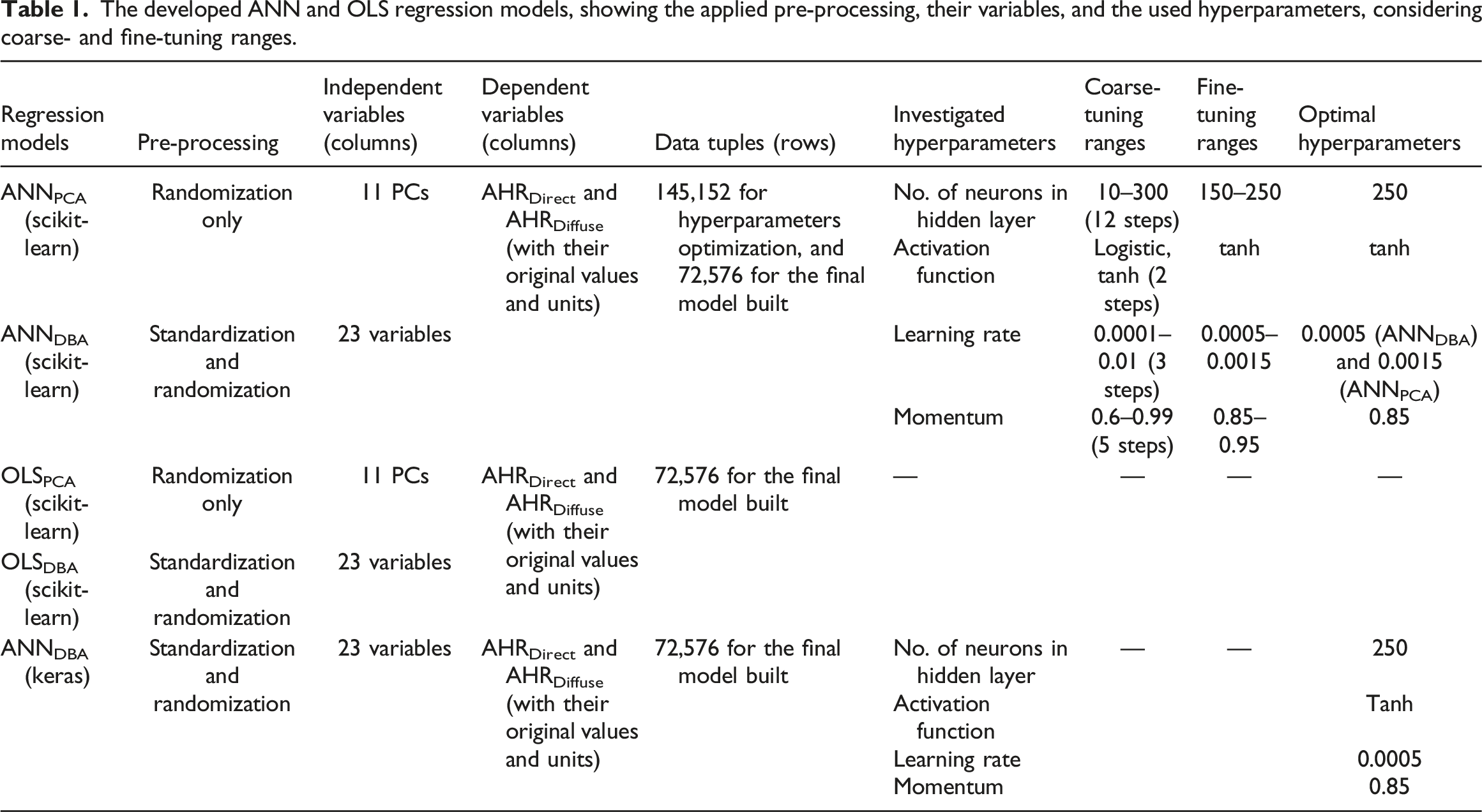
Ordinary least-squares regression considered Barrel, Groin, and Cloister VRFs only, whereas their variations, Pointed Barrel, Pointed Groin, and Pointed Cloister, were employed to perform TL. DB_PCA that included 13 columns and only 72,576 rows, along with DB_DBA without PCA that included 25 columns and 72,576 rows as well, were used to build two OLS models, namely, OLS_PCA and OLS_DBA, respectively (Table 1). Scikit-learn was used to fit those OLS models by linear approximation that minimized the SSE between the original observations and predictions made by those models. However, the performance evaluation of OLS, along with ANN, is discussed in the Performance Evaluation section.

Table 1.

The developed ANN and OLS regression models, showing the applied pre-processing, their variables, and the used hyperparameters, considering coarse- and fine-tuning ranges.

Regression models	Pre-processing	Independent variables (columns)	Dependent variables (columns)	Data tuples (rows)	Investigated hyperparameters	Coarse-tuning ranges	Fine-tuning ranges	Optimal hyperparameters
ANN_PCA (scikit-learn)	Randomization only	11 PCs	AHR_Direct and AHR_Diffuse (with their original values and units)	145,152 for hyperparameters optimization, and 72,576 for the final model built	No. of neurons in hidden layer	10–300 (12 steps)	150–250	250
ANN_PCA (scikit-learn)	Randomization only	11 PCs			Activation function	Logistic, tanh (2 steps)	tanh	tanh
ANN_DBA (scikit-learn)	Standardization and randomization	23 variables			Learning rate	0.0001–0.01 (3 steps)	0.0005–0.0015	0.0005 (ANN_DBA) and 0.0015 (ANN_PCA)
ANN_DBA (scikit-learn)	Standardization and randomization	23 variables			Momentum	0.6–0.99 (5 steps)	0.85–0.95	0.85
OLS_PCA (scikit-learn)	Randomization only	11 PCs	AHR_Direct and AHR_Diffuse (with their original values and units)	72,576 for the final model built	—	—	—	—
OLS_DBA (scikit-learn)	Standardization and randomization	23 variables		72,576 for the final model built	—	—	—	—
ANN_DBA (keras)	Standardization and randomization	23 variables	AHR_Direct and AHR_Diffuse (with their original values and units)	72,576 for the final model built	No. of neurons in hidden layer	—	—	250
					Activation function			Tanh
					Learning rate			0.0005
					Momentum			0.85

Artificial neural networks

Similar to OLS, ANN considered Barrel, Groin, and Cloister VRFs only. Scikit-learn was used to create 2 feedforward ANN models based on DB_PCA and DB_DBA, namely, ANN_PCA and ANN_DBA, respectively (Table 1), to investigate their performance using hyperparameters optimization. Their initial architecture included input, hidden, and output layers (Figure 9). ANN_PCA and ANN_DBA were trained via the optimization algorithm of stochastic gradient-descent¹⁰¹ to estimate the error gradient of models’ current state using examples from the training data, where the weights got updated by backpropagation. Different hyperparameters were investigated to iteratively refine the developed models against their prediction accuracy. They included the number of neurons in hidden layer, activation function that introduces non-linear properties to ANNs,³⁵ learning rate that defines the update rate of weights to minimize errors during the training, and momentum that simplify and accelerate the progress of the training.

Figure 9.

The implemented ANN architecture, showing different layers and the investigated activation function.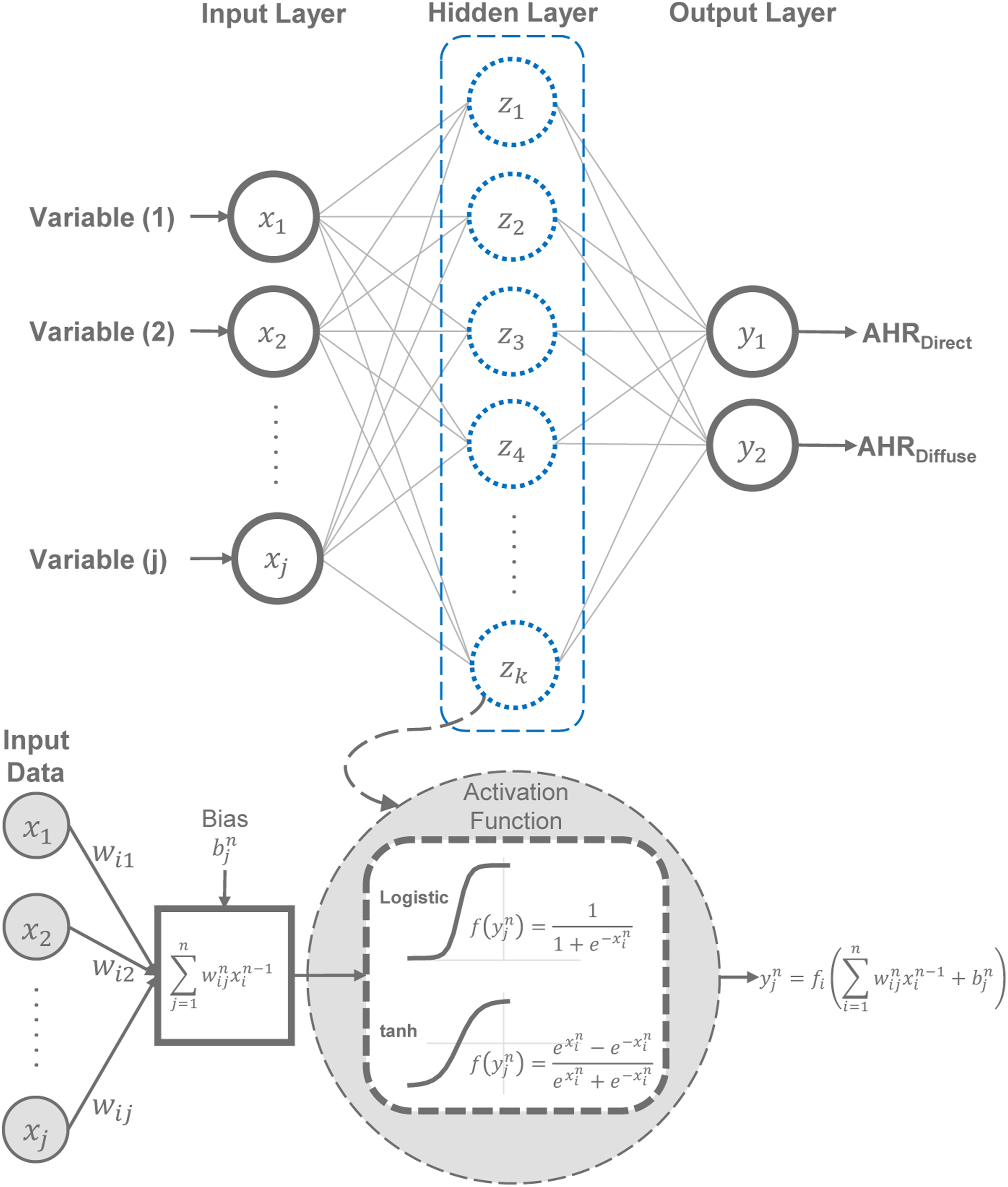

Hyperparameters optimization

The training and testing of ANN models were conducted through the pre-defined four steps. First, data was split by K-Fold cross-validation and brought into trainable range. Before building the models, DS_DBA was randomized, then standardized, while DS_PCA was randomized only because it was standardized before. Data standardization was conducted by scikit-learn’s Standard Scaler. Then, each dataset was split into two parts, 80% for training and 20% for testing, where the training data was further split into five subsets, representing new training and validation data. ANN_PCA and ANN_DBA were trained iteratively 5 times on alternating four folds, then validated on the remaining fold. A grid search was carried out in hyperparameters coarse-tuning, where wider bounds of search space was defined then examined to narrow down the investigation (Table 1). A set of curves were created to explore the quality of training and validation against hyperparameters, yielding 1800 combinations for each ANN_PCA and ANN_DBA (12 numbers of neurons in hidden layer × two activation functions × three learning rates × five momentums × five Folds). (Figure 10) shows grid search results, according to training (blue lines) and validation (red lines) accuracies. RMSE results of those curves were close to each other. As expected, training curves exhibited relatively less prediction errors than validation curves, since the models could perform better on data that they already saw during training. The results of ANN_DBA model had marginally less RMSE than ANN_PCA because the latter was built from vertically reduced 11 PCs that explain only 92.28% of DS_DBA; but was fitted with less computations.

Figure 10.

The results of hyperparameters coarse-tuning for ANN_PCA and ANN_DBA, showing (a) number of neurons in hidden layer, (b) activation function, (c) learning rate, and (d) momentum.

Looking at the training and validation curves of different hyperparameters, it can be concluded that the number of neurons in the hidden layer is inversely proportional to the error rate (Figure 10(a)). ANN_PCA having 150–250 neurons in the hidden layer obtained less RMSE of 26.40–23.11 for training and 26.71–23.56 for validation, compared to other numbers of neurons in the hidden layer. ANN_DBA of the same number of neurons obtained smaller RMSE of 21.24–19.91 for training and 21.73–20.55 for validation. Still, the curves of ANN_DBA showed that both curves plateaued after 250 neurons for training with RMSE of 19.28 and validation of 20.00. For activation function, (Figure 10(b)) confirmed that ANN_PCA and ANN_DBA employing tanh yielded less RMSE of 22.00 and 18.62 for training and 22.11 and 18.78 for validation, respectively, supported by different K-folds of similar behavior. ANN_PCA and ANN_DBA using logistic yielded RMSE of 23.43 and 20.28 for training and 23.54 and 20.43 for validation, respectively. Again, (Figure 10(c) and (d)) revealed that ANN_PCA having 0.001 learning rate and 0.90 momentum yielded lowest RMSE of 44.04 and 44.36 for training and 44.27 and 44.58 for validation, respectively, compared to the other hyperparameters. ANN_DBA of the same learning rate and momentum obtained lesser RMSE values of 37.45 and 37.87 for training and 37.80 and 38.21 for validation. Such hyperparameters were deemed optimal for ANN models, and their neighboring values were further examined in fine-tuning (Table 1).

To trace the results of fine-tuning, the third step entails developing two convergence plots for ANN_PCA and ANN_DBA (Figure 11). Using BO with maximum number of iterations of 50, both plots illustrated how RMSE varied during every iteration of training (blue lines) and validation (red lines), considering the selected optimal hyperparameters. Similar to coarse-tuning, the fine-tuning convergence plots showed that the training and validation curves were close, but training yielded less error than validation. Overall, the results of ANN_DBA obtained less errors than ANN_PCA. The best performing ANN_PCA is having 250 neurons in the hidden layer, 0.0015 learning rate, and 0.85 momentum, which obtained RMSE of 19.03 for training and 19.49 for validation. The best performing ANN_DBA is having 250 neurons in the hidden layer, 0.0005 learning rate, and 0.85 momentum, which obtained acceptable RMSE of 16.47 for training and 17.10 for validation. Thus, ANN_DBA model with these optimal hyperparameters was deemed the best-performing model. PCA did not bring much improvement to ANN modeling from the overall accuracy perspective. The results confirmed that the developed model from the selected input variables yielded more accurate prediction without requiring additional PCA.

Figure 11.

Hyperparameters fine-tuning results of ANN_PCA and ANN_DBA. (a) Convergence plot of ANN_PCA. (b) Convergence plot of ANN_DBA.

Performance evaluation

Training and testing of OLS models were conducted by initially bringing the data into trainable range and order. DS_DBA was randomized and standardized by scikit-learn’s Standard Scaler. DS_PCA was standardized before, thus, was only randomized. Then, each dataset was split into two parts, 80% for training and 20% for testing. As stated before, the developed OLS_PCA and OLS_DBA considered Barrel, Groin, and Cloister VRFs. Testing data was compared against the acquired predictions from OLS_PCA (Figure 12(a) and (c)) and OLS_DBA (Figure 12(b) and (d)), in terms of RMSE and R². They were illustrated by scatter plots of AHR_Direct and AHR_Diffuse observations on x-axis and their corresponding predictions on y-axis, assessing them against a 45-degree line. For AHR_Direct and AHR_Diffuse, OLS_PCA obtained inadequate R² values of 33.714 and 51.585%, with large RMSE of 177.055 and 41.202, respectively. OLS_DBA also obtained inadequate R² of 37.666 and 63.155%, with less RMSE of 171.693 and 35.943, respectively. The scatter plots showed that the results of both models did not reflect good fitting between observations and predicted values. This was confirmed by large RMSE values, where a set of residual analysis was plotted to visualize the difference between AHR_Direct and AHR_Diffuse observations and their respective predictions from both models. This analysis proved the unsuitability of the developed OLS models to fit the data.

Figure 12.

Prediction results, showing scatter plots of AHR_Direct and AHR_Diffuse observations against their corresponding predictions of the developed (a) OLS_PCA and (b) OLS_DBA models. Residual analysis is also illustrated, showing the difference between AHR_Direct and AHR_Diffuse observations against their corresponding predictions of (c) OLS_PCA and (d) OLS_DBA models.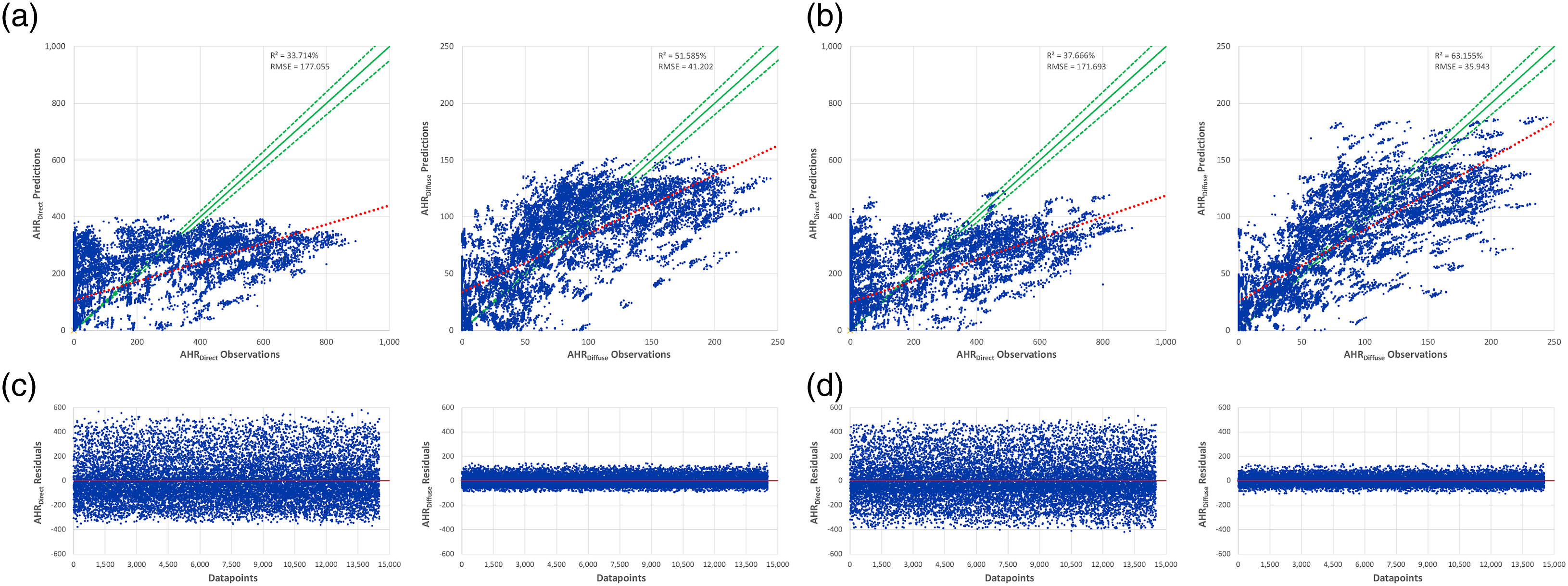

Regarding ANN, once satisfied with the training and validation of the optimized hyperparameters, DS_PCA and DS_DBA, considered Barrel, Groin, and Cloister VRFs, were used to develop ANN_PCA and ANN_DBA models with their optimized hyperparameters in the last step. The unseen testing data observations were compared against the obtained predictions from both ANN_PCA (Figure 13(a) and (c)) and ANN_DBA (Figure 13(b) and (d)). The results were illustrated by scatter plots of AHR_Direct and AHR_Diffuse observations on x-axis and their corresponding predictions on y-axis. For AHR_Direct and AHR_Diffuse, ANN_PCA obtained good R² values of 98.249 and 95.599%, with RMSE of 28.790 and 12.437, respectively. ANN_DBA obtained even better accuracy results with R² of 98.773 and 96.749%, with lesser RMSE of 24.167 and 10.683, respectively. To confirm the validity of the developed models, a set of residual analysis was conducted by plotting the difference between AHR_Direct and AHR_Diffuse observations and their respective predictions from both models. Compared to OLS models, these tests confirmed the suitability of the developed ANN models to fit the data. Without clear patterns, the random distribution of residuals above and below the zero-axis shows that ANN_DBA is performing very well, and it was a good choice for such dataset.

Figure 13.

Prediction results, showing scatter plots of AHR_Direct and AHR_Diffuse observations against their corresponding predictions of the developed (a) ANN_PCA and (b) ANN_DBA models. Residual analysis is also illustrated, showing the difference between AHR_Direct and AHR_Diffuse observations against their corresponding predictions of (c) ANN_PCA and (d) ANN_DBA models.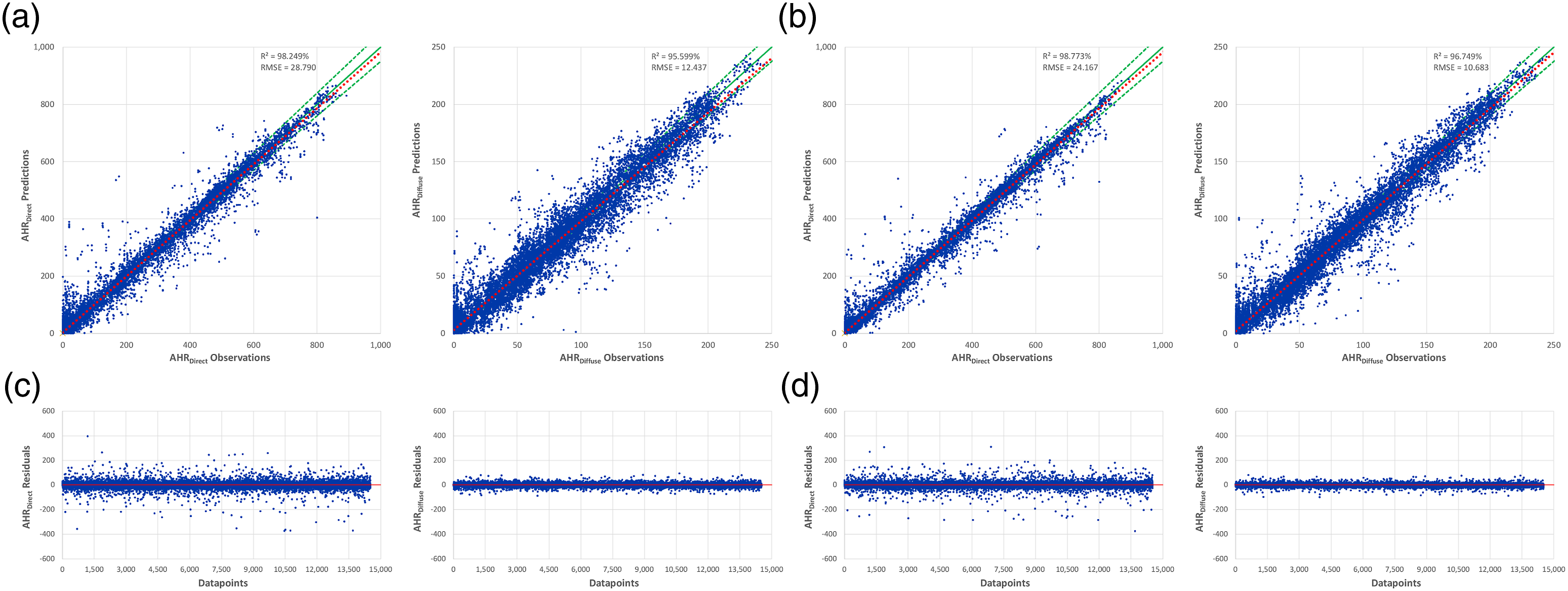

Overall, OLS models obtained much larger error rates than ANN models. This was expected, because of the involved non-linearity of training and testing datasets. OLS_PCA was the worst-performing model, followed by OLS_DBA, because the former was trained using vertically reduced 11 PCs that explain only 92.28% of DS_DBA. OLS relies on minimizing RSS without regularization that penalizes complex models. Inversely, the used activation function offered ANN models with non-linear attributes, making them perform better than OLS, although they did not benefit from vertical reduction of data.

Transfer learning

Considering Barrel, Groin, and Cloister VRFs, DS_DBA was used to develop an additional ANN_DBA model in keras with the same optimal hyperparameters that were obtained by scikit-learn (Table 1). To assess its accuracy, testing observations were compared against the obtained predictions from the model (Figure 14(a) and (c)). The results were shown via scatter plots of AHR_Direct and AHR_Diffuse observations on x-axis and their related predictions on y-axis. ANN_DBA (keras) obtained very similar performance patterns to ANN_DBA (scikit-learn), with R² of 98.794 and 97.889%, and RMSE of 23.909 and 8.412, respectively. These results were confirmed by a set of residual analysis, showing the difference between AHR_Direct and AHR_Diffuse observations and predictions from ANN_DBA (keras). Without clear patterns, the random distribution of residuals uncovered that the model is comparably performing well. It was found useful to compare the predictions of AHR_Direct and AHR_Diffuse, that were obtained from both ANN_DBA (keras) and ANN_DBA (scikit-learn) (Figure 14(b) and (d)). The results showed a high association between both models, with strong positive R² of 99.263 and 97.978%, and minimal RMSE of 18.680 and 8.340, respectively. This suggested that the changes in ANN_DBA (keras) predictions correspond to equivalent variations in ANN_DBA (scikit-learn) in the same direction.

Figure 14.

Prediction results, showing scatter plots of AHR_Direct and AHR_Diffuse observations against their corresponding predictions of the developed (a) ANN_DBA model (keras) and (b) ANN_DBA model (scikit-learn) vs ANN_DBA model (keras). Residual analysis is also illustrated, showing the difference between AHR_Direct and AHR_Diffuse observations against their corresponding predictions of (c) ANN_DBA (keras) model and (d) ANN_DBA model (scikit-learn) vs ANN_DBA model (keras).

Once satisfied with the performance of ANN_DBA (keras), it was extracted to manipulate its architecture. The first input layer and the earlier trained weights and biases of the hidden layer were frozen. The last output layer was replaced with a new one to present new predictions (Figure 15). Such layers were utilized to construct a new feedforward model for TL, ANN_TL, with similar optimal hyperparameters (Table 1). The new output layer was trained using new training data of Pointed Barrel Vaults, Pointed Groin Vaults, and Pointed Cloister VRFs that were extracted from the original DS_Sim, including 25 columns and 2,207,520 rows. This data was brought into trainable range and order by standardization and randomization. Then, DS_Sim was split into two parts, 97.5% for training and only 2.5% for testing, representing a sufficient fraction of DS_Sim to conduct an adequate training of ANN_TL.

Figure 15.

The new ANN architecture, showing the kept and removed layers, along with the added output layer.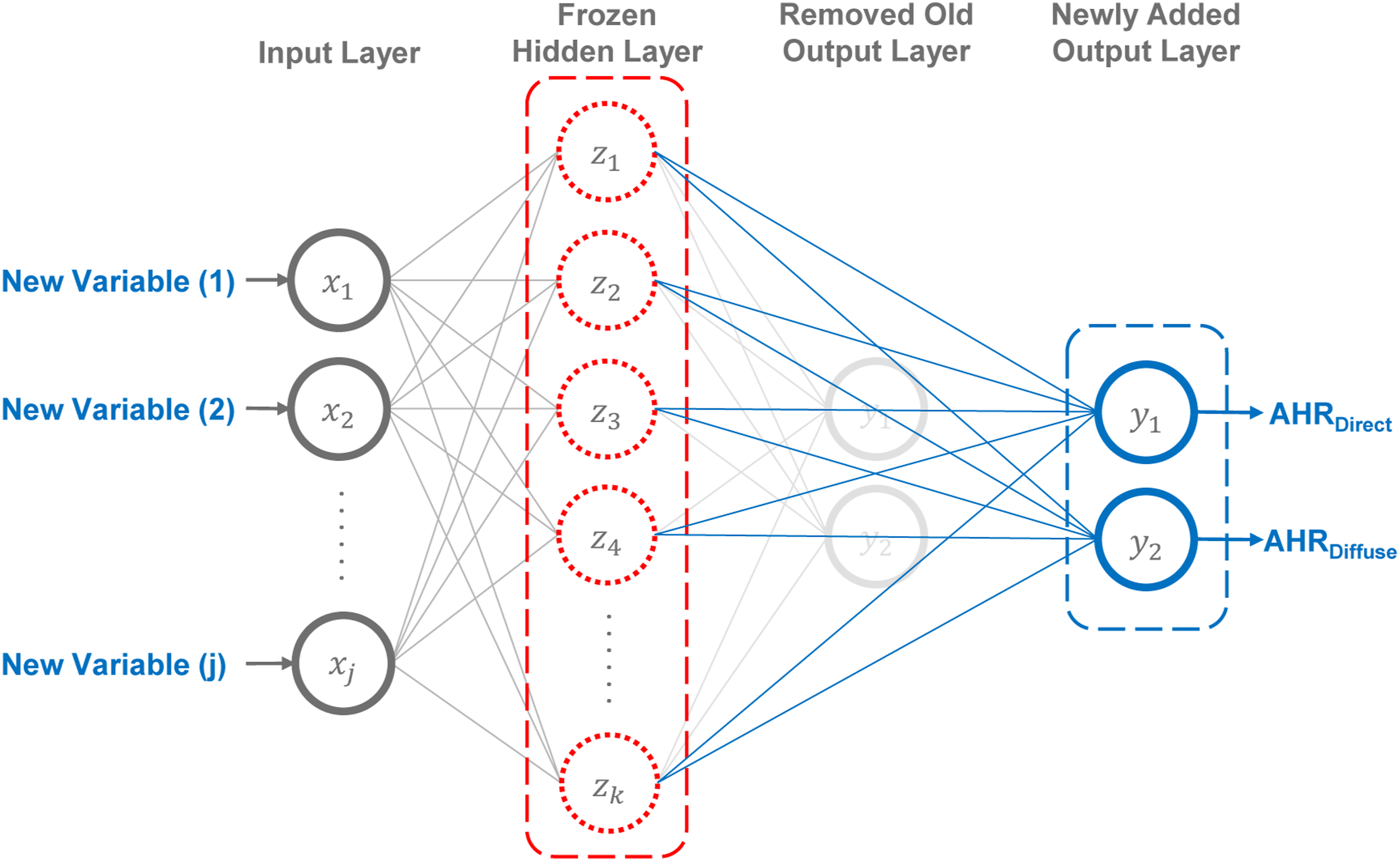

To evaluate the accuracy of ANN_TL, the testing data observations were compared against the obtained predictions from the model (Figure 16(a)). The results were illustrated by scatter plots of AHR_Direct and AHR_Diffuse observations on x-axis and their related predictions on y-axis. For AHR_Direct and AHR_Diffuse, ANN_TL yielded adequate R² values of 87.416 and 94.713%, with acceptable RMSE of 79.300 and 13.971, respectively. The availability of DS_Sim gives the opportunity to assess the performance ANN_DBA (keras) to predict Pointed variations of VRFs. The testing data observations were also compared against predictions from ANN_DBA (keras) (Figure 16(b)). The results were analyzed by scatter plots of AHR_Direct and AHR_Diffuse observations on x-axis against their corresponding predictions on y-axis. The ANN_DBA model obtained very poor R² values of 17.335 and 37.748%, with larger RMSE of 203.247 and 77.399 for both AHR_Direct and AHR_Diffuse, respectively.

Figure 16.

Prediction results, showing scatter plots of AHR_Direct and AHR_Diffuse observations against their corresponding predictions of the developed (a) ANN_TL model (keras) and (b) ANN_DBA model (keras).

Overall, ANN_DBA model acquired much larger error rates than ANN_TL. This was expected, because the former made predictions from data that was outside its training area, leading to increased error rates. This suggests that newly input data from other VRFs cannot be used as-is, confirming the importance of TL. The strength of the developed ANN_TL that made satisfactory predictions, although not excellent, encourages exploiting it as a proxy to predict the solar performance of VRFs in the early stages of design. TL can be utilized to predict the performance of diverse VRFs by leveraging minor datasets from similar roof forms.

Conclusion

This research highlighted three research trendlines of varying complexity that focused on investigating the solar performance of CRFs. With limited landscape of related research attempts, the reviewed studies demonstrated the ability of CRFs to reduce the received intensities of solar irradiance, compared to flat roofs. Most recent attempts relied on simulations to obtain quantifications on how well CRFs would perform under different conditions. Still, this approach is inherently time-consuming and computationally demanding, hindering to rapidly acquire preliminary approximations during the early design stages.

The work of this research represented an unprecedented attempt to investigate the potential contribution of two regression MLAs to rapidly provide preliminary approximations on the received solar irradiance by six VRFs, with reference to the hot-desert climate of Aswan, Egypt. Supported by additional validation, simulation-derived datasets were generated, pre-processed, trained, and tested to create MLA models. While PCA has indeed been widely utilized for feature extraction and reduction in various fields, its application in the context of estimating the received solar irradiances by traditional VRFs has not been extensively explored. This study innovatively integrates PCA within the framework of machine learning algorithms to extract hidden information and reveal correlations among variables specific to the solar performance of traditional vaulted roofs. Compared to OLS, the results verified the ability of ANN models to precisely estimate solar irradiances, with adequate R² of 96.573–98.741% and insignificant RMSE of 10.566–24.525 Wh/m². The research also considered another interesting possibility to transfer the learned knowledge of the best-performing model and apply them to predict new VRFs. The ability of the transferred models to accurately estimate solar irradiances was confirmed, with R² of 88.337–94.449% and RMSE of 14.317–76.342 Wh/m².

This research bears the challenging viability of exploiting MLAs, which comes with the cost of acquiring sufficient training and testing data that are often simulation-derived or directly monitored from buildings. As a part of reinforcement learning, inventive application of artificial intelligence, called Neuroevolution, presents itself as new methodology that combines using evolutionary (genetic) algorithms to derive the generation of many ANNs with varying architectures and parameters. The practicality of Neuroevolution arises from its ability to replace supervised MLAs that require large datasets, as input-output pairs for training and testing, with measures of ANNs’ performance, allowing them to evolve and mutate. This way, Neuroevolution separates itself from ANN with fixed architectures that depend on conventional gradient-descent. The results can be measured without requiring numerical or labeled examples of the anticipated outcomes.

In the era of artificial intelligence, a paradigm shift is taking place in the field of architecture. Architects are now beginning to move away from being “conventional practitioners,” only to find themselves “half-programmers” who incorporate MLAs to blur the demarcation between traditional and contemporary practices. This change arises from the necessity to put forward passive solutions for reducing energy use for cooling and improving indoor thermal conditions in buildings. Indeed, MLAs are relatively easy to exploit by architects as pre-diagnostic tools for building performance estimation, without performing exhaustive simulations. Even for practitioners who lack the knowledge about environmental analysis, MLAs can help addressing the variations of different parameters during the conceptual stage. Moreover, MLAs can guide decision-makers identifying potential strategies for future developments, offering predictions for setting regulations of newly built contexts.

Footnotes

Declaration of conflicting interests

The author(s) declared no potential conflicts of interest with respect to the research, authorship, and/or publication of this article.

Funding

The author(s) received no financial support for the research, authorship, and/or publication of this article.

ORCID iD

Mohammed Ayoub

References

Taleb

. Using passive cooling strategies to improve thermal performance and reduce energy consumption of residential buildings in UAE buildings. Front Archit Res 2014; 3: 154–165.

Fahmy

Mahdy

Nikolopoulou

. Prediction of future energy consumption reduction using GRC envelope optimization for residential buildings in Egypt. Energy Build 2014; 70: 186–193.

Soleimani

Calautit

Hughes

. Computational Analysis of natural ventilation flows in geodesic dome building in hot climates. Computation 2016; 4: 31.

Ayoub

Elseragy

. Parameterization of traditional domed-roofs insolation in hot-arid climates in Aswan, Egypt. Energy Environ 2018; 29: 109–130.

Elnokaly

Ayoub

Elseragy

. Parametric investigation of traditional vaulted roofs in hot-arid climates. Renew Energy 2019; 138: 250–262.

Sirimanna

MPG

Attalage

. A model for analyzing the thermal performance of roof configurations with flat inclined surfaces. Energy Build 2016; 116: 122–132.

Tang

Meir

. Thermal performance of non air-conditioned buildings with vaulted roofs in comparison with flat roofs. Build Environ 2006; 41: 268–276.

Ramzy

. Sustainable spaces with psychological values: historical architecture as reference book for biomimetic models with biophilic qualities. ArchNet-IJAR 2015; 9: 248–267.

Fathy

. Natural energy and vernacular architecture: principles and examples with reference to hot arid climates. Chicago, IL: University of Chicago Press, 1986.

10.

Olgyay

. Design with climate: bioclimatic approach to architectural regionalism. Princeton, NJ: Princeton University Press, 1973.

11.

Konya

. Design primer for hot climate. London, UK: The Architectural Press Ltd, 1980.

12.

Mainstone

. Developments in structural form. New York, NY: MIT Press, 1983.

13.

Pearlmutter

. Roof geometry as a determinant of thermal behaviour: a comparative study of vaulted and flat surfaces in a hot-arid zone. Archit Sci Rev 1993; 36: 75–86.

14.

Elseragy

. Architectural and solar potential of curved and flat roofs in hot arid regions, with reference to Egypt. Nottingham, UK: University of Nottingham, 2003.

15.

Gómez-Muñoz

Porta-Gándara

MÁ

Heard

. Solar performance of hemispherical vault roofs. Build Environ 2003; 38: 1431–1438.

16.

Hadavand

Yaghoubi

. Thermal behavior of curved roof buildings exposed to solar radiation and wind flow for various orientations. Appl Energy 2008; 85: 663–679.

17.

Hadavand

Yaghoubi

Emdad

. Thermal analysis of vaulted roofs. Energy Build 2008; 40: 265–275.

18.

Runsheng

Meir

Etzion

. An analysis of absorbed radiation by domed and vaulted roofs as compared with flat roofs. Energy Build 2003; 35: 539–548.

19.

Tang

Meir

Etzion

. Thermal behavior of buildings with curved roofs as compared with flat roofs. Sol Energy 2003; 74: 273–286.

20.

Faghih

Bahadori

. Solar radiation on domed roofs. Energy Build 2009; 41: 1238–1245.

21.

Faghih

Bahadori

. Thermal performance evaluation of domed roofs. Energy Build 2011; 43: 1254–1263.

22.

Parkhurst

Darringer

Grundmann

. From single core to multi-core: preparing for a new exponential. In: IEEE/ACM international conference on computer-aided design, digest of technical papers, San Jose, CA, 05–09 November 2006, ICCAD, pp. 67–72.

23.

Koomey

Berard

Sanchez

, et al. Implications of historical trends in the electrical efficiency of computing. IEEE Ann Hist Comput 2011; 33: 46–54.

24.

Ayoub

. 100 years of daylighting: a chronological review of daylight prediction and calculation methods. Sol Energy 2019; 194: 360–390.

25.

Ward

. The RADIANCE lighting simulation and rendering system. Orlando, FL: ACM Press, 1994.

26.

Rutten

. Grasshopper. Seattle, WA: Robert McNeel and Associates, 2022.

27.

Jakubiec

Reinhart

. DIVA 2.0: integrating daylight and thermal simulations using Rhinoceros 3D, Daysim and EnergyPlus. In: Proceedings of the international building simulation association conference, Sydney, NSW, 14–16 November 2011, pp. 2202–2209.

28.

Ayoub

. Contrasting accuracies of single and ensemble models for predicting solar and thermal performances of traditional vaulted roofs. Sol Energy 2022; 236: 335–355.

29.

Marion

William

Urban

Ken

. User’s Manual for TMY2s (Typical Meteorological Years)-Derived from the 1961-1990 National Solar Radiation Data Base. No. NREL/TP-463-7668. Colorado, USA: National Renewable Energy Lab.(NREL), 1995.

30.

NSRD . 1991–2005 update: typical meteorological year 3. https://rredc.nrel.gov/solar/old_data/nsrdb/1991-2005/tmy3/ (2020, accessed 1 November 2020).

31.

ASHRAE . International weather files for energy calculations 2.0 (IWEC2). https://www.ashrae.org/technical-resources/bookstore/ashrae-international-weather-files-for-energy-calculations-2-0-iwec2 (2019, accessed 2 October 2019).

32.

Perez

Seals

Michalsky

. All-weather model for sky luminance distribution-preliminary configuration and validation. Sol Energy 1993; 50: 235–245.

33.

Uetani

CIE , et al. Spatial Distribution of Daylight - CIE Standard General Sky. Vienna, Austria: International Commission on Illumination (CIE), 2003.

34.

Ayoub

. A multivariate regression to predict daylighting and energy consumption of residential buildings within hybrid settlements in hot-desert climates. Indoor Built Environ 2019; 28: 848–866.

35.

Ayoub

. A review on machine learning algorithms to predict daylighting inside buildings. Sol Energy 2020; 202: 249–275.

36.

Ibarra

Reinhart

. Daylight factor simulations-how close do simulation beginners ‘really’ get? Proceedings of building simulation 2009: 11th conference of IBPSA, Glasgow, Scotland, 27–30 July 2009, pp. 196–203.

37.

Mitchell

. Machine learning. New York, NY: McGraw-Hill Higher Education, 1997.

38.

Zhou

Liu

. Prediction of daylighting and energy performance using artificial neural network and support vector machine. Am J Civ Eng Archit 2015; 3: 1–8.

39.

Yoon

Moon

Kim

. Development of annual daylight simulation algorithms for prediction of indoor daylight illuminance. Energy Build 2016; 118: 1–17.

40.

Lorenz

Jabi

. Predicting daylight autonomy metrics using machine learning. In: Proceedings of the international conference for sustainable design of the built environment (SDBE 2017), London, UK, December 20-21, 2017, pp. 991–1002.

41.

Kazanasmaz

Günaydin

Binol

. Artificial neural networks to predict daylight illuminance in office buildings. Build Environ 2009; 44: 1751–1757.

42.

López

Gueymard

. Clear-sky solar luminous efficacy determination using artificial neural networks. Sol Energy 2007; 81: 929–939.

43.

Pattanasethanon

Lertsatitthanakorn

Atthajariyakul

, et al. An accuracy assessment of an empirical sine model, a novel sine model and an artificial neural network model for forecasting illuminance/irradiance on horizontal plane of all sky types at Mahasarakham, Thailand. Energy Convers Manag 2008; 49: 1999–2005.

44.

Tang

Lee

, et al. Classification of CIE standard skies using probabilistic neural networks. Int J Climatol A J R Meteorol Soc 2010; 30: 305–315.

45.

Janjai

Plaon

. Estimation of sky luminance in the tropics using artificial neural networks: modeling and performance comparison with the CIE model. Appl Energy 2011; 88: 840–847.

46.

Lou

. Review of solar irradiance and daylight illuminance modeling and sky classification. Renew Energy 2018; 126: 445–453.

47.

Zhang

Shi

, et al. Enhancing diffusion MRI measures by integrating grey and white matter morphometry with hyperbolic Wasserstein distance. IEEE/CAA J Autom Sin 2017; 2017: 520–524.

48.

Chen

Liu

, et al. Estimation of monthly solar radiation from measured temperatures using support vector machines–a case study. Renew Energy 2011; 36: 413–420.

49.

Zou

Wang

Lin

, et al. Estimation of global solar radiation using an artificial neural network based on an interpolation technique in southeast China. J Atmos Sol Terr Phys 2016; 146: 110–122.

50.

Lou

Lam

. CIE standard sky classification by accessible climatic indices. Renew Energy 2017; 113: 347–356.

51.

Bellocchio

Ferrari

Lazzaroni

, et al. Illuminance prediction through SVM regression. In: IEEE workshop on Environmental energy and structural monitoring systems (EESMS), Milan, Italy, 28 September 2011, pp. 1–5.

52.

Şahin

Oğuz

Büyüktümtürk

. Approximate and three-dimensional modeling of brightness levels in interior spaces by using artificial neural networks. J Electr Eng Technol 2015; 10: 1822–1829.

53.

Yadav

Chandel

. Solar radiation prediction using artificial neural network techniques: a review. Renew Sustain Energy Rev 2014; 33: 772–781.

54.

Voyant

Notton

Kalogirou

, et al. Machine learning methods for solar radiation forecasting: a review. Renew Energy 2017; 105: 569–582.

55.

Zendehboudi

Baseer

Saidur

. Application of support vector machine models for forecasting solar and wind energy resources: a review. J Clean Prod 2018; 199: 272–285.

56.

Ramadhan

Heatubun

Tan

, et al. Comparison of physical and machine learning models for estimating solar irradiance and photovoltaic power. Renew Energy 2021; 178: 1006–1019.

57.

Lou

Lam

, et al. Prediction of diffuse solar irradiance using machine learning and multivariable regression. Appl Energy 2016; 181: 367–374.

58.

Geiger

. Klassifikation der Klimate nach W. Köppen. Landolt-Börnstein – Zahlenwerte und Funktionen aus Physik, Chemie, Astronomie, Geophysik und Technik, Alte Serie. Berlin, Germany: Springer, 1954, pp. 603–607.

59.

Critchfield

. Criteria for classification of major climatic types in modified Köppen system. Idaho, USA: University of Idaho, 1983.

60.

Kottek

Grieser

Beck

, et al. World map of the Köppen-Geiger climate classification updated. Metz 2006; 15: 259–263.

61.

EnergyPlus . Weather data. EnergyPlus documentation. US Department of Energy (DOE), 2020, https://energyplus.net/weather.

62.

Duffie

Beckman

. Solar engineering of thermal processes. 3rd ed. New York, USA: John Wiley and Sons, 2006.

63.

Elseragy

Elnokaly

. Assessment criteria for form environmental performance of building envelope in hot arid climates. In: The passive and low energy architecture 24th international conference PLEA 2007, Singapore, 22–24 November 2007, pp. 156–162.

64.

Elseragy

Gadi

. Computer simulation of solar radiation received by curved roof in hot-arid regions. In: The 8th international IBPSA conference, Eindhoven, Netherlands, 11–14 August 2003, pp. 11–14.

65.

Ayoub

. Self-organizing profiles to characterize representative temporal settings for daylight simulations. Sol Energy 2021; 214: 248–267.

66.

Levermore

Parkinson

. Analyses and algorithms for new test reference years and design summer years for the UK. Build Serv Eng Res Technol 2006; 27: 311–325.

67.

Charles

Crawley

. Weather data for building performance simulation. In: Hensen

Lamberts

(eds). Building performance simulation for design and operation. New York, NY: Spon Press, 2011, pp. 37–55.

68.

Wei

. Predictions of surface solar radiation on tilted solar panels using machine learning models: a case study of Tainan city, Taiwan. Energies 2017; 10: 1660.

69.

Sarbu

Sebarchievici

. Thermal energy storage. Solar heating and cooling systems - fundamentals, experiments and applications. Cambridge, MA: Academic Press, 2017, pp. 99–138.

70.

ASHRAE . ASHRAE handbook of HVAC applications. Atlanta, GA: American Society of Heating, Refrigerating and Air-Conditioning Engineers, 2007.

71.

Leondes

. Computer techniques and algorithms in digital signal processing. Advances in theory and applications. Amsterdam, Netherlands: Elsevier, 1996.

72.

Morel

Achard

Kulpa

, et al. Time-series averaging using constrained dynamic time warping with tolerance. Pattern Recognit 2018; 74: 77–89.

73.

Berndt

Clifford

. Using dynamic time warping to find patterns in time series. In: Proceedings of the 3rd international conference on knowledge discovery and data mining, Anchorage, AK, 4–8 August 2019, pp. 359–370.

74.

Wang

Zhao

Wang

, et al. Effects of exposure to a 50 Hz sinusoidal magnetic field during the early adolescent period on spatial memory in mice. Bioelectromagnetics 2013; 34: 275–284.

75.

Petitjean

Ketterlin

Gançarski

. A global averaging method for dynamic time warping, with applications to clustering. Pattern Recognit 2011; 44: 678–693.

76.

Petitjean

. DBA.py. 2018, https://github.com/fpetitjean/DBA/blob/master/DBA

77.

Wold

Esbensen

Geladi

. Principal component analysis. Chemom Intell Lab Syst 1987; 2: 37–52.

78.

Jolliffe

. Principal component analysis. 2nd ed. New York, NY: Springer-Verlag, 2002.

79.

Viviani

Grön

Spitzer

. Functional principal component analysis of fMRI data. Hum Brain Mapp 2005; 24: 109–129.

80.

Kalkstein

Tan

Skindlov

. An evaluation of three clustering procedures for use in synoptic climatological classification. J Clim Appl Meteorol 1987; 26: 717–730.

81.

Lam

Wan

Wong

, et al. Principal component analysis and long-term building energy simulation correlation. Energy Convers Manag 2010; 51: 135–139.

82.

Platon

Dehkordi

Martel

. Hourly prediction of a building’s electricity consumption using case-based reasoning, artificial neural networks and principal component analysis. Energy Build 2015; 92: 10–18.

83.

Chatterjee

Hadi

Price

. Regression analysis by example. 3rd ed. New York, NY: John Wiley and Sons, 2000.

84.

Hecht-Nielsen

. Theory of the backpropagation neural network. In: Wechsler

(ed). Neural Networks for perception. Cambridge, MA: Academic Press, 1992, pp. 65–93.

85.

Jain

Mao

Mohiuddin

. Artificial neural networks: a tutorial. Computer (Long Beach Calif) 1996; 29: 31–44.

86.

Bishop

. Pattern recognition and machine learning. Singapore: Springer, 2006.

87.

Rumelhart

Hinton

Williams

. Learning representations by back-propagating errors. Nature 1986; 323: 533–536.

88.

Pedregosa

Varoquaux

Gramfort

, et al. Scikit-learn: machine learning in python. J Mach Learn Res 2011; 12: 2825–2830.

89.

Trenn

. Multilayer perceptrons: approximation order and necessary number of hidden units. IEEE Trans Neural Netw 2008; 19: 836–844.

90.

Snoek

Larochelle

Adams

. Practical Bayesian optimization of machine learning algorithms. In: Proceedings of the 25th international conference on neural information processing systems, Lake Tahoe, NV, 3–6 December, 2012, pp. 2951–2959.

91.

Masters

. Practical neural network recipes in C++. Cambridge, MA: Morgan Kaufmann Publishers, 1993.

92.

Injadat

Salo

Nassif

, et al. Bayesian optimization with machine learning algorithms towards anomaly detection. In: Proceedings of IEEE Global Communications Conference, Abu Dhabi, UAE, 09–13 December 2018, pp. 1–6.

93.

Mockus

. Bayesian approach to global optimization: theory and applications. Berlin, Germany: Springer Science and Business Media, 2012.

94.

Zhu

. Hyper-parameter optimization: a review of algorithms and applications. 2003. arXiv:2003.05689.

95.

Rasmussen

. Gaussian processes in machine learning. In Proceedings of summer school on machine learning. Berlin, Germany: Springer, 2003, pp. 63–71.

96.

Head

Kumar

Nahrstaedt

, et al. Scikit-optimize. 2020; Epub ahead of print 2020. DOI: 10.5281/zenodo.4014775.

97.

Weiss

Khoshgoftaar

Wang

. A survey of transfer learning. J Big Data 2016; 3: 1–40.

98.

Chollet

. Keras. 2015, https://keras.io

99.

Cerda

Varoquaux

Kégl

. Similarity encoding for learning with dirty categorical variables. Mach Learn 2018; 107: 1477–1494.

100.

Van Loan

. Computational frameworks for the fast Fourier transform. Philadelphia, PA: Society for Industrial and Applied Mathematics, 1992.

101.

Bottou

. Stochastic gradient descent tricks. Neural networks: tricks of the trade. Berlin, Germany: Springer, 2012, pp. 421–436.