An Introduction to Multilevel Regression and Post-Stratification for Estimating Constituency Opinion

Abstract

This article provides an overview of multilevel regression and post-stratification. It reviews the stages in estimating opinion for small areas, identifies circumstances in which multilevel regression and post-stratification can go wrong, or go right, and provides a worked example for the UK using publicly available data sources and a previously published post-stratification frame.

Keywords

small area estimation multilevel regression and post-stratification public opinion Bayesian methods R

Introduction

Multilevel regression and post-stratification (MRP) is a technique for estimating public opinion in small areas using large national samples. ‘Small areas’ are usually anything smaller than nations, and past work using MRP has produced estimates for areas as large as US states (average population: 6.5 million) to areas as small as Westminster constituencies (average population: 100,000) (Hanretty et al., 2018; Park et al., 2004). ‘Large samples’ also vary in size, and depend on the context: some MRP work (typically work producing estimates for a small number of small areas) has used national samples of around 1500 (Leemann and Wasserfallen, 2017), while some very large work in election forecasting has used samples of more than 80,000 (Lauderdale et al., submitted).

Researchers and practitioners use MRP because they are interested in subnational opinion. Different people can be interested in subnational opinion for different reasons. Political scientists tend to be interested in subnational opinion because they are interested in whether subnational opinion is reflected in legislatures. Election forecasters are interested in subnational opinion because in many electoral systems national vote shares are a poor good to relevant electoral outcomes. Others still may be interested in subnational opinion for commercial reasons.

MRP is used because the alternatives are either very poor or very expensive. A poor alternative is simply splitting a large sample into (much) smaller geographic subsamples. This is a poor alternative because there is no guarantee that a sample which is representative at the national level will be representative when it is broken down into smaller groups. This approach is also only possible when the number of respondents per small area is relatively large. Lax and Phillips (2009a) combine four different national surveys on same sex marriage into a ‘mega-poll’ of 6458. The expected number of respondents per state is therefore around 130. Splitting up a large sample is a plausible strategy with this many respondents per state. It would not be plausible for estimating opinion in the 435 congressional districts (expected respondents per area: 15).

An expensive alternative is conducting polls in each small area for which we want to estimate public opinion. This strategy is possible where the number of small areas is relatively small. Most of the 50 US states are large enough to support state polling companies. It would be possible, though expensive, to conduct surveys in each of these states. It would not, however, be feasible to conduct a survey in each of the 650 Westminster constituencies: any research design which involves surveying more than half a million people is probably beyond the reach of any private concern.

Because these alternatives are often not possible or not desirable, and because MRP is now an established technique, many researchers are curious about the analyses MRP makes possible. There is therefore a need for a guide which sets out, in practical terms, the issues involved in producing MRP estimates of opinion for small areas, and which provides a template for such analyses.

This document tries to provide such a template. I begin by describing the history of MRP, before describing the principal stages in any MRP analysis. I then set out the scope of MRP, the design considerations, and other practical issues relating to implementation. I finally provide code and a worked example for researchers working in the UK.

The History of MRP

The basic idea behind MRP is that it is possible to group people into different types based on their sociodemographic characteristics, and to make predictions for each of those types on the basis of an appropriate statistical model. These predictions can then be used to make estimates for small areas if we can use or generate information on how many voters of each type are present in each area.

This basic idea emerged in the 1960s (see the discussion in Park et al. (2004)), but it was not until the early 2000s when statistical modelling techniques were sufficiently well-developed to make MRP feasible for (advanced) applied researchers. A methodological paper by Park et al., 2004 was quickly followed by substantive applications in the United States (Lax and Phillips, 2009b; Warshaw and Rodden, 2012). MRP methods were subsequently applied in the UK (Hanretty et al., 2018), Switzerland (Leemann and Wasserfallen, 2017) and (in a slightly different form) Germany (Selb and Munzert, 2011).

Since that time, development of MRP as a method has focusing on how to use the richest possible post-stratification frames (Lauderdale et al., submitted; Leemann and Wasserfallen, 2017) and how to ensure that the multilevel regression models employ as rich and as extensive a range of predictor variables as possible (Ghitza and Gelman, 2013; Goplerud et al., 2018).

Stages in Estimating Local Opinion Using MRP

There are four stages which must be carried out when conducting an analysis of local opinion using MRP:

Conduct or compile survey information which contains information on respondents’ opinions regarding some political or social issue, and information on respondents’ background characteristics, and information on which small area the respondent lives in;

Compile information on relevant characteristics of the small areas in questions;

Estimate a multilevel regression model using the information from the first and second stages;

Obtain or construct a post-stratification frame which contains information on the joint distribution of respondent background characteristics by small area;

Make predictions from the multilevel regression model estimated in stage 3 for each row in the post-stratification frame, and aggregate these predictions to the level of the small area;

Getting the Survey Information

Estimates of opinion in small areas has to be based on survey responses. Researchers may be in the fortunate position of being able to commission original survey research. Or, researchers may have access to the raw data from an existing large survey. Finally, researchers may have access to several smaller surveys which they can combine.

If researchers are commissioning an original survey, they will be able to specify both what background characteristics are recorded, and how they are recorded. Researchers will want to ensure that background characteristics are recorded in ways that either match the post-stratification frame, or can be recoded so as to match. Sometimes this can be difficult. In the UK, information on educational attainment is often provided according to NVQ Levels, where Level 4 is equivalent to a post-secondary qualification, Level 3 is equal to the highest type of secondary qualification, and so on. Almost no one knows about these categories, and so respondents must instead be asked whether they have a university degree, or A-levels, or other named qualifications, and these responses must be recoded to match the different NVQ levels.

Any researcher commissioning an original survey will have to give thought to the necessary sample size. The answer to the question ‘how large a sample is required?’ is almost always ‘the largest you can afford’. More practically, the answer will depend on the number of small areas for which estimates are required. Kastellec et al. (2016) report that MRP produces ‘reasonably accurate estimates of [US] state public opinion using as little as a single large national poll–approximately 1,400 survey respondents’, or 28 respondents per small area. The required number of respondents will increase with the number of small areas, but it will increase at a lower rate than this. Hanretty et al. (2017) created estimates of attitudes to same-sex marriage and general left-right orientation for the 632 constituencies in Great Britain using information from between 8000 and 12,000 respondents, or between 13 and 19 respondents per small area.

A more common situation is where researchers have information from an existing large national survey. The British Election Study online panel has information from a very large number of respondents. Because it is a general purpose social scientific study, it also contains information on a large number of respondent characteristics, including characteristics that could be used in post-stratification. Researchers do, however, need to recode the information from the BES so that the values of BES variables match the values of variables in the post-stratification frame.

If researchers do not have access to a single large sample, but only multiple smaller samples, then this work of recoding variables becomes much more difficult. Where the samples have been collected at different times or using different methods, researchers may need to model these extra factors, and pick a ‘preferred’ method and time for the purposes of post-stratification.

Getting the Constituency Information

Very often descriptions of MRP do not discuss the process of gathering constituency information. This is unfortunate. The accuracy of MRP estimates can be more strongly affected by the inclusion of good constituency predictors than by the details of the post-stratification frame (Buttice and Highton, 2013; Toshkov, 2015: 459). Fortunately, researchers in the UK can benefit from the resources compiled by the British Election Studies team, who include a very helpful database of constituency-level information.

The choice of constituency variables to include will be guided by the opinion being modelled, and by the variables that previous research has identified as mattering for that opinion. Occasionally, compiling this information can be difficult if different sub-units of a country report information in different ways. The proportion of the population without a passport was a strong local-authority level predictor of the Leave vote in the 2016 EU referendum – but this information, derived in England and Wales from the 2011 census, is not available for Scottish constituencies.

Estimating the Model

Most researchers will be familiar with regression models, which I define as any model which tries to relate measures of a dependent variable, or outcome, to measures of one or more independent variables, or predictor variables, by means of an equation. Regression models exist for outcomes of various types (continuous outcomes, dichotomous outcomes, categorical outcomes), and in principle if you can model an outcome using a regression model, you can produce estimates of that outcome as part of MRP. (In practice, categorical outcomes can be tricky: Kastellec et al. (2015: 792))

Multilevel regression models are models where the parameters in the model apply to different levels. In MRP models, these levels are usually hierarchically organised. That is, the model uses information about respondents (level 1 information), but also information about the small areas in which respondents are located (level 2 information), and possibly also information about broader groupings of small areas like regions (level 3 information).

One key part of MRP models is the effect associated with each small area, which some researchers describe as a random intercept.¹ These constituency effects are drawn from a common distribution. This allows for small area estimates to be idiosyncratic, given what we know and can measure about the people who live in them and their other characteristics. Crucially, it allows for these idiosyncrasies to borrow strength from one another. Because random intercepts are drawn from a common distribution, information about a different small area can affect our estimate of the effect associated with one respondent’s area. If evidence from another area suggests that the effect associated with that area is very large, it can mean that the distribution of area effects generally contains very large values. This might in turn mean that we estimate a larger value of the area effect for the area we started with.

Multilevel regression is common enough to feature in most statistical environments, but complex enough to present some difficulties in implementation. In addition, since multilevel regression for the purposes of MRP is often estimated through Bayesian methods, researchers who only know about frequentist methods will have to familiarise themselves with a different terminology.

Getting the Post-Stratification Frame

In the context of MRP, a post-stratification frame is a large rectangular data frame which contains, for each small area, all the possible combinations of respondent characteristics, together with either the count or the proportion of residents of each area who have those characteristics.

For example, the post-stratification frame used in Hanretty et al. (2018) contains information on the proportion of constituency residents according to gender (male/female), housing tenure (rents/owns), sector of the economy (private/public), marital status (married/not married), age group (eight different groupings), educational level (six different groupings), and social grade (four different groupings). There are therefore 3072 (2×2×2×2×8×6×4) voter types for each constituency, and 1.9 million (3072 × 632) rows in the data.

It is much easier to use an existing post-stratification frame than it is to construct one oneself. The construction of post-stratification frames has become more complicated over time, and the state of the art involves not just combining several different sources of information, but also running complicated imputation models, and using techniques (like raking, or iterative proportional fitting) familiar to survey researchers but not familiar to applied social scientists.

The first applications of MRP were able to use existing ‘analytic’ post-stratification frames made available by Census authorities. For example, Park et al. (2004) modelled presidential vote choice using four individual-level characteristics: sex, ethnicity (African-American or other), age (four categories), and education (four categories). The 1990 US Census provided the joint distribution of these four variables (‘we know from the census that there were 66,177 adults who lived in Alabama, were male, not black, aged 18–29, and did not have a high school diploma’). Census authorities can release this relatively detailed information at the level of US states because the total numbers in each cell are still large.

Where the number of individual level variables is larger, or where the ‘small areas’ are smaller, it is not possible to use these ‘analytic’ post-stratification frames. For example, the most complicated UK Census tables available at constituency level are three-way tables (e.g. approximated social grade by sex by age, Table LC6124EW).

Consequently, researchers have turned to ‘synthetic’ (researcher-created) joint distributions. These synthetic distributions can be produced in simple or elaborate ways. The simple way of producing a joint distribution is to use information on the marginal distributions of variables (which Census authorities do release at small area level), and assume that these variables are independent. Thus, the proportion of women who are aged 25–34 is equal to the proportion of women, times the proportion of people aged 25–34. This is a poor way of producing joint distributions, because important social and political variables are often associated with one another. In the UK, the proportion of people aged 55–64 with a university degree is substantially lower than the proportion of people aged 55–64 times the proportion of people with a university degree, because university education has become more popular over time. However, Leemann and Wasserfallen (2017) were able to show (by simulation and example) that if we are interested only in the small area estimate, then these errors in the joint distribution tend to cancel out.

The elaborate way of producing a joint distribution for each small area is to take some existing joint distribution (perhaps the joint distribution at national level, or the joint distribution from the survey), and ‘rake’ these joint distributions to match the known marginal distribution at the level of the small area. Earlier research stuck with Census information. Hanretty et al. (2018), for example, took information from the Census Sample of Anonymised Records, and raked these to the known constituency marginal distributions (see Appendix B of Hanretty et al., 2018).

Perhaps emboldened by Leemann and Wasserfallen (2017), more recent research has started with joint distributions which include non-Census variables like past vote behaviour, and has raked to the constituency results of recent elections. For example, Lauderdale et al. (submitted) created a post-stratification frame for the 2017 general election which included information on 2015 vote, 2016 vote, age, qualifications, and gender.

Making Predictions and Aggregating

If researchers are able to estimate a model, and able to obtain a post-stratification frame, then the last stage should be comparatively easy. All that is required is to generate predicted values for each row in the post-stratification frame using the parameter values from the estimated regression model. These might be predicted probabilities (for a dichotomous outcome) or predicted values (for a continuous outcome). These predicted values can then be multiplied by the proportion given in the post-stratification frame, and added together to give the proportion or count at the level of the constituency.

Where estimates of uncertainty are required (and estimates of uncertainty are always useful) then predicted values can be repeatedly generated using different draws from the posterior distribution of the model.

In principle, multilevel regression and post-stratification could be used to generate an estimate of opinion for the country as a whole, rather than for multiple small areas. Multilevel regression and post-stratification would therefore perform the same function as sample weighting, but would allow more complicated sets of variables to be used as ‘weights’. Some researchers have had success in using MRP in this way to correct for samples known to be unrepresentative. In principle, MRP could also be used to generate estimates of other arbitrary combinations of respondent characteristics. It would be possible to generate estimates for young home-owners, or Labour leavers, or other groups.

When Does MRP Go Wrong, and When Does It Go Right?

Questions Which Pick Out Different Things in Different Areas

Sometimes, surveys asks questions about named individuals or named organisations. If respondents to a survey are asked for their opinion on Theresa May, we can be fairly confident that they have in mind the same person, rather than some other person who happens to share the name of the Conservative Prime Minister.

Where respondents have in mind the same object, we can assume that their opinions are governed by the same process. Individual respondents may have very different views about Theresa May, but any particular respondent’s view would change in the same way if (counterfactually) they aged 10 years, or changed gender, or relocated to a majority-Conservative constituency.

Sometimes, however, surveys ask questions in ways that lead respondents to picture different individuals or organisations. Surveys might ask about rates of satisfaction with ‘your local MP’, or ‘your local police service’. It would be wrong to model these kinds of opinions using MRP, because the same process would not govern the responses given. In some areas, having voted Conservative in the last election would cause you to be more favourable towards your local MP; in other areas (most obviously, constituencies not held by the Conservative party), it would cause you to be less favourable towards your local MP.

There are borderline cases between these two extremes. Levels of trust in one’s local MP might be satisfactorily modelled using MRP, if we are prepared to claim that trust is a general personality disposition which is strongly affected by respondent characteristics, and which extends to local MPs without being strongly affected by their party label.

Unpredictable Beliefs

MRP can also go wrong when it is used to model unpredictable beliefs. In order for MRP to work, the opinion in question has to be credibly related to constituency and/or individual-level variables. Opinion regarding Theresa May can credibly be related to both constituency and individual level variables, because Theresa May is a Conservative party politician; attitudes towards Conservative party politicians are strongly structured by attitudes to the Conservative party, and these in turn are strongly structured by different social and constituency characteristics.

It would not be possible in the same way to model beliefs about the authorship of Shakespeare’s plays, not just because few people have attitudes about the authorship of Shakespeare’s plays, but because even among those people who do have strong opinions regarding Edward de Vere or Christopher Marlowe, these opinions are not obviously structured by social or constituency characteristics.

There are many cases in between these two extremes: attitudes in relation to some supermarkets, or some other types of popular culture, for example, might be strongly structured by education and class. It is hard to say in advance when the relationship is sufficiently strong to enable MRP to be carried out. In the case of the example given later, estimates which are on the face of it plausible can be constructed even when the individual level model offers a relatively poor fit to the data.

Rare Outcomes

One particular issue with MRP has emerged quite clearly in the context of election forecasting. Generally, it is difficult to use MRP to provide estimates of opinions held with low frequency (less than 1% to 2%). This may result from attenuation bias (Lauderdale et al., submitted), or from general difficulties in explaining rare events with logistic regression models (King and Zeng, 2001).

Non-Representative Samples

MRP can do well given some kinds of non-representative samples, and can do poorly when given other kinds of non-representative samples. Whether MRP does well or poorly depends on the ways in which the sample is non-representative.

If the sample is non-representative because certain characteristics are over- (under-)represented, and those characteristics are included in the post-stratification frame, then MRP can do well. Wang et al. (2015) used data from a survey of Xbox users to predict the results of the 2012 presidential election. Xbox users are not a representative sample of the population: they are much younger, and much more likely to be male. However, those demographic characteristics are present in most post-stratification frames.

If the sample is non-representative because certain characteristics are over- (under-represented), and those characteristics are not included in the post-stratification frame, then MRP will not do well. For example, suppose that an online panel has much higher levels of political interest than the general population, and that higher levels of interest are positively associated with the belief we want to study. MRP will therefore over-estimate the prevalence of the belief in question at the level of the small area, for just the same reason that a national poll would over-estimate the prevalence of the belief at the national level.

MRP can therefore be regarded as a functional equivalent to survey weighting. Like survey weighting, it depends on the variables used, the relationship between those variables and the opinion being modelled, and the relationship between unmeasured variables and the opinion being modelled.

When Demography is Destiny

I noted earlier that MRP will fail to generate good estimates of local opinion when it is asked to model unpredictable beliefs. The converse is also true: MRP will do well when asked to model very predictable beliefs. This is particularly true where demographic characteristics have a very strong relationship with the outcome in question.

The recent EU membership referendum in the UK is a good example of this. Voting behaviour in the referendum was strongly affected by education: individuals with higher educational qualifications were more likely to vote to Remain. This relationship held at both the individual and aggregate level. Because of this, even relatively simple multilevel models, which included no post-stratification element, did well, and not much less than much more complicated models (Lauderdale et al., submitted).

When There is a Past Benchmark

In the case of the EU membership referendum, there was no good past benchmark for opinion on EU membership. The previous 1975 referendum on the UK’s membership of the European Community was too long ago and counted on different boundaries. For general elections, however, past results provide a very good benchmark as to the relative ordering of constituencies. This is the reason why uniform national swing works well.

MRP models of vote behaviour therefore generally include lagged versions of party vote share as a small area level predictor. More recent MRP work has moved to using past party choice as an individual level predictor. In this way, MRP builds not just on uniform national swing, but on the alternative approach of using transition matrices (McLean, 1973). Some MRP models can therefore make claims like ‘x% of Labour Leavers stuck with the party in 2017’.

When Good and Abundant Constituency Predictors are Used

Several authors have already noted how good constituency predictors can improve the accuracy of MRP estimates considerably (Buttice and Highton, 2013; Hanretty et al., 2018; Toshkov, 2015: 459). Despite this, relatively few constituency predictors are used. This is particularly perplexing where the number of small areas is large. Consider the British case. If we were estimating a linear regression of party vote share, then one popular rule of thumb (Harrell, 2014) would suggest that we could estimate up to 62 coefficients, or 1 coefficient for every 10 constituencies. Yet applications often use far fewer constituency-level predictors, between 6 (Hanretty et al., 2018) and 14 (Lauderdale et al., submitted). This may be because we are already estimating 632 constituency coefficients drawn from a common distribution.

A Worked Example

In this section, I describe how to provide constituency-level estimates of 0–10 left-right self-placement, using as survey data wave 13 of the 2015–2017 British Election Study, and using as post-stratification data a cut-down version of the post-stratification data used in Hanretty et al. (2018). I have used both of these data sources because they are already in the public domain. I have used a cut-down version of the post-stratification data in Hanretty et al. (2018) because the variables I removed are either not commonly available in many data-sets (private/public sector employment) or have become more complicated to code over time (marital status). I have chosen a continuous variable to demonstrate the technique because it allows me to make claims about the proportion of variance explained using a commonly understood metric (R²).

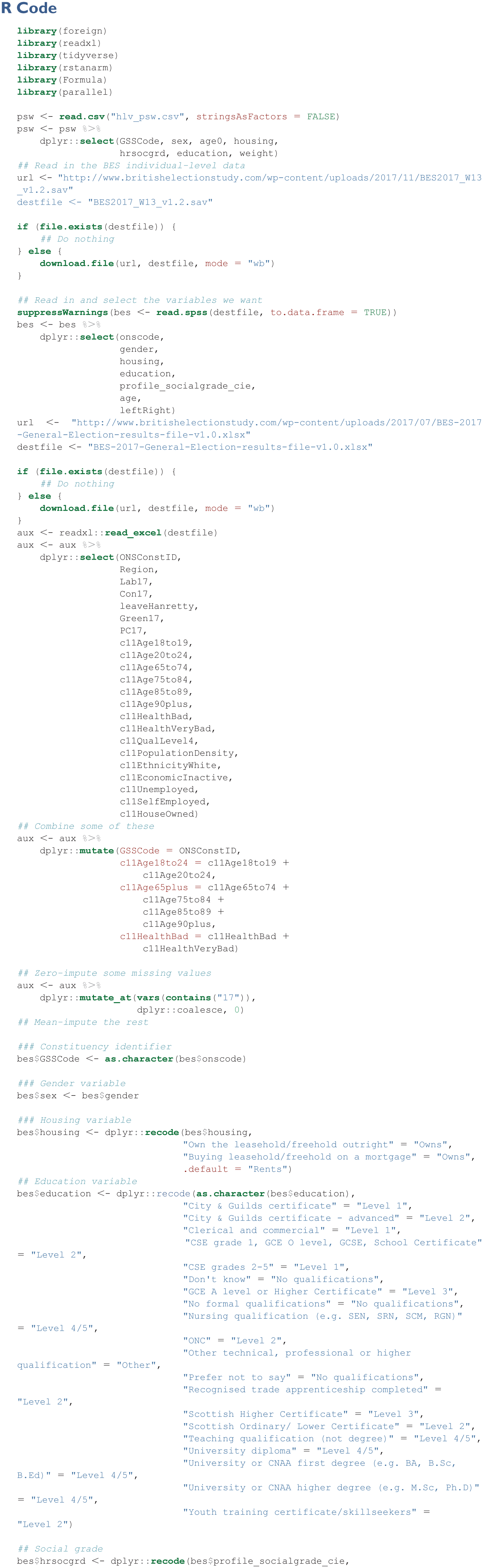
The worked example uses R code. Most of the code reported in the appendix deals with tidying the data and ensuring the variables in the BES match the category found in the post-stratification data. The estimates are produced by calling a function (mrp) contained in a separate source file. That function in turn calls functions from the rstanarm package, which is a wrapper around the Stan programming language.

The first chunk loads some of the R packages necessary for the script. Libraries foreign and readxl are used to load in the survey and auxiliary data, respectively. The tidyverse package is used to aid in recoding the data. The rstanarm package has already been described. The Formula package is used to handle two-part formulae (individual level predictors and area level predictors). Finally, the parallel package allows multiple Monte Carlo chains to be estimated using multiple cores (where these exist).

The second code chunk reads in the post-stratification data. The post-stratification data contain information on the constituency variable (GSSCode), together with information on sex, age, housing tenure, social grade, and education. The variable weight records the proportion in each constituency who match the values of the variables present in each row.

The third code chunk loads the data from wave 13 of the BES, and selects the necessary variables. The fourth code chunk loads the auxiliary data supplied by the BES team, and selects some variables which have proven useful in modelling. The fifth code chunk is the longest, and involves recoding variables from the BES so that their values (or names) match the values (names) found in the post-stratification frame. This can involve combining categories (education, housing), discretizing them (age), or simply renaming them.

The last lines of the code chunk remove incomplete cases. A large number of observations are dropped because they lack information on housing. If this were not a teaching example, we would want to explore the patterns of missingness, and investigate models of imputing missing data conditional on other characteristics. As it is, dropping incomplete observations shrinks the total number of observations to 12,026, speeding up the time taken to estimate the model.

The sixth code chunk actually carries out the estimation. It begins by specifying a two-part formula. The part before the tilde identifies the dependent variable. The part after the tilde, but before the vertical bar identifies variables present in the post-stratification data. The part after the vertical bar identifies constituency variables.

After setting up the function to use multiple cores where they exist, we call the function mrp. This function takes as arguments a two-part formula, names of data frames (the separate survey, post-stratification, and auxiliary data-frames), and a character vector giving the name of the variable holding the constituency identifiers. Because we are modelling a continuous outcome, we specify type = ‘continuous’. Finally, we specify the name of the variable in the post-stratification data frame holding the post-stratification weights.

All of the other arguments are passed to the stan_glmer function in the rstanarm package. Of particular importance are the arguments specifying the number of iterations in the initial warm up stage, together with the number of iterations in total, including any iterations in the warm-up phase. The larger these numbers, the longer the estimation will take. On my 2017 laptop with a quad-core processor clocked at 2.50 Ghz, estimation took around 90 minutes using these settings. These settings are probably the shortest desirable run. For final estimates, total iterations of around 1000 per chain would be preferable.

Generally, rstanarm will give appropriate warnings where the chains are too short, or where the sampler explores the parameter space poorly. Sometimes, these warnings can be disregarded. In this example, rstanarm gives a warning that there was ‘one [or more] divergent transition[s]’ after warm-up – but small numbers of divergent transitions (less than then) can often be ignored. Once again, for final estimates, a longer number of warm-up and total iterations may be desirable.

The results from the mrp command are stored in an object. The command print.mrp will show the top and bottom five. The results themselves are stored in res$constsmry$intervals. Some manipulation may be necessary to convert ONS constituency codes to human-readable names.

## MRP estimation of variable: leftRight

## Model formula:

## leftRight ~ sex + age0 + housing + hrsocgrd + education | Con17 + Lab17 +

Region +

## leaveHanretty + Green17 + PC17 + c11Age18to24 + c11Age65plus + c11HouseOwned +

## c11SelfEmployed + c11Unemployed + c11EconomicInactive +

c11EthnicityWhite +

## c11PopulationDensity + c11QualLevel4 + c11HealthBad

## Respondents: 12026. Mean squared error: 10.39

## Top five

## ===

## 1) Christchurch: 6.2 [5.9, 6.5]

## 2) Clacton: 6 [5.7, 6.3]

## 3) Castle Point: 5.9 [5.6, 6.2]

## 4) New Forest West: 5.9 [5.6, 6.1]

## 5) Rayleigh and Wickford: 5.8 [5.6, 6]

## Bottom five

## ===

## 628) Hackney South and Shoreditch: 3.5 [3.3, 3.8]

## 629) Islington North: 3.5 [3.2, 3.8]

## 630) Sheffield Central: 3.5 [3.2, 3.8]

## 631) Hackney North and Stoke Newington: 3.5 [3.2, 3.8]

## 632) Liverpool, Riverside: 3.4 [3.1, 3.7]

The (standardised) coefficients from the model are stored in res$fit, which is an rstanarm object which can be interrogated using the many functions available for that package. Of particular interest in this case is the bayes_R2 function, which shows that the R-squared for this analysis is just 0.12. This is a summary statistic for the individual level model; the correlation between the MRP estimates and the true (unknown) constituency opinion can be high even where the individual-level model is poor. Obviously constituency opinion is more likely to be estimated well when the individual model offers a good fit to the data.

Conclusion

MRP is a technique which has been in active development for the past 15–20 years. It has made it possible to pose and answer many questions related to public opinion in small areas which have not been possible before.

There have been three main obstacles to more widespread use of MRP. First, MRP requires experience of multilevel regression and often requires some familiarity with Bayesian methods. Both of these are more common now than they used to be. Second, MRP is computationally intensive, particularly where the number of observations is high and where post-stratification frame is large. These computational burdens continue to be an obstacle – MRP cannot be fit in a matter of seconds – but are less severe than before. Third, MRP requires assembling a number of different sources of data, not all of which are easy to work with.

The present article, in supplying code and data necessary to undertake these kinds of analyses for the UK, can deal with the third of these problems. However, researchers interested in using MRP for their own analyses should ensure that they have some familiarity with what is happening ‘under the hood’.

Supplemental Material

article – Supplemental material for An Introduction to Multilevel Regression and Post-Stratification for Estimating Constituency Opinion

Supplemental material, article for An Introduction to Multilevel Regression and Post-Stratification for Estimating Constituency Opinion by Chris Hanretty in Political Studies Review

This article is distributed under the terms of the Creative Commons Attribution 4.0 License (http://www.creativecommons.org/licenses/by/4.0/) which permits any use, reproduction and distribution of the work without further permission provided the original work is attributed as specified on the SAGE and Open Access pages (https://us-sagepub-com-s.web.bisu.edu.cn/en-us/nam/open-access-at-sage).

Supplemental Material

hlv_psw – Supplemental material for An Introduction to Multilevel Regression and Post-Stratification for Estimating Constituency Opinion

Supplemental material, hlv_psw for An Introduction to Multilevel Regression and Post-Stratification for Estimating Constituency Opinion by Chris Hanretty in Political Studies Review

Supplemental Material

mrp – Supplemental material for An Introduction to Multilevel Regression and Post-Stratification for Estimating Constituency Opinion

Supplemental material, mrp for An Introduction to Multilevel Regression and Post-Stratification for Estimating Constituency Opinion by Chris Hanretty in Political Studies Review

Footnotes

Declaration of Conflicting Interests

The author declared the following potential conflicts of interest with respect to the research, authorship, and/or publication of this article: During the period in which this manuscript was written, the author carried out consultancy work for the polling company Survation, which uses MRP in its work. The author continues to work for Survation in this capacity, but does not hold shares in Survation or any other polling company.

Funding

The author received no financial support for the research, authorship, and/or publication of this article.

ORCID iD

Chris Hanretty

Data Accessibility Statement

Replication code for this article can be found at the Harvard Dataverse: .

Notes

Author Biography

Chris Hanretty is a Professor of Politics at Royal Holloway, University of London. He carries out research on public opinion and representation, and on courts and how judges behave. He is a recipient of the Phillip Leverhulme Prize (for researchers ‘whose work has had international impact and whose future research career is exceptionally promising’) and the Richard Rose Prize (for ‘a distinctive contribution to British politics’).

References

Buttice

Highton

(2013) How Does Multilevel Regression and Poststratification Perform With Conventional National Surveys? Political Analysis 21 (4): 449–467.

Gelman

Hill

(2006) Data Analysis Using Regression and Multilevel/Hierarchical Models. Cambridge: Cambridge university press.

Ghitza

Gelman

(2013) Deep Interactions With MRP: Election Turnout and Voting Patterns Among Small Electoral Subgroups. American Journal of Political Science 57 (3): 762–776.

Goplerud

Kuriwaki

Ratkovic

, et al. (2018) Sparse Multilevel Regression (and Poststratification (sMRP)). Working paper, Harvard University, Cambridge, MA.

Hanretty

Lauderdale

Vivyan

(2017) Dyadic Representation in a Westminster System. Legislative Studies Quarterly 42 (2): 235–267.

Hanretty

Lauderdale

Vivyan

(2018) Comparing Strategies for Estimating Constituency Opinion From National Survey Samples. Political Science Research and Methods 6 (3): 571–591.

Harrell

(2014) Regression Modeling Strategies. Berlin: Springer.

Kastellec

Lax

Phillips

(2016) Estimating State Public Opinion With Multi-level Regression and Poststratification Using R. Available at: http://www.princeton.edu/~jkastell/MRP_primer/mrp_primer.pdf

Kastellec

Lax

Malecki

, et al. (2015) Polarizing the Electoral Connection: Partisan Representation in Supreme Court Confirmation Politics. The Journal of Politics 77 (3): 787–804.

10.

King

Zeng

(2001) Logistic Regression in Rare Events Data. Political Analysis 9 (2): 137–163.

11.

Lauderdale

Blumenau

Rivers

(submitted) Model-Based Pre-Election Polling for National and Sub-National Outcomes in the US and UK. International Journal of Forecasting.

12.

Lax

Phillips

(2009a) Gay Rights in the States: Public Opinion and Policy Responsiveness. American Political Science Review 103 (3): 367–386.

13.

Lax

Phillips

(2009b) How Should We Estimate Public Opinion in the States? American Journal of Political Science 53 (1): 107–121.

14.

Leemann

Wasserfallen

(2017) Extending the Use and Prediction Precision of Subnational Public Opinion Estimation. American Journal of Political Science 61 (4): 1003–1022.

15.

McLean

(1973) The Problem of Proportionate Swing. Political Studies 21 (1): 57–63.

16.

Park

Gelman

Bafumi

(2004) Bayesian Multilevel Estimation With Poststratification: State-Level Estimates From National Polls. Political Analysis 12 (4): 375–385.

17.

Selb

Munzert

(2011) Estimating Constituency Preferences From Sparse Survey Data Using Auxiliary Geographic Information. Political Analysis 19 (4): 455–470.

18.

Toshkov

(2015) Exploring the Performance of Multilevel Modeling and Poststratification With Eurobarometer Data. Political Analysis 23 (3): 455–460.

19.

Wang

Rotschild

Goel

, et al. (2015) Forecasting Elections With Non-Representative Polls. International Journal of Forecasting 31 (3): 980–991.

20.

Warshaw

Rodden

(2012) How Should We Measure District-Level Public Opinion on Individual Issues? The Journal of Politics 74 (1): 203–219.

Supplementary Material

Please find the following supplemental material available below.

For Open Access articles published under a Creative Commons License, all supplemental material carries the same license as the article it is associated with.

For non-Open Access articles published, all supplemental material carries a non-exclusive license, and permission requests for re-use of supplemental material or any part of supplemental material shall be sent directly to the copyright owner as specified in the copyright notice associated with the article.

0.00 MB

0.01 MB

37.25 MB

0.05 MB