Doping,the Inspection Game,and Bayesian Enforcement

Introduction

This article analyzes whether doping enforcers, who are benevolent, but make imperfect decisions, can prevent doping. Doping enforcers are not perfectly informed about the actual past behavior of an athlete. Instead, they have to rely on erroneous doping tests. They are, however, not blind, as they are able to uncover the actual behavior better than by pure chance. Hence, they are “imperfect decision makers.” ¹ Through the examination of a case and, in particular, through doping tests, they generate an informative signal which is correlated with what the athlete has actually done. ²

Another property that characterizes the doping enforcer in this article is their “benevolence.” First, the enforcer is assumed to prefer a higher social welfare and, thus, is interested in avoiding welfare losses. Second, the enforcer is assumed to prefer correct judgments over incorrect ones. ³ The second assumption reflects their preference for justice. ⁴ The idea that doping leads to a welfare loss does not, at first glance, seem to be true, if only the interests of the athletes are taken into account, because a victory based on doping would do nothing else but shift some utility from one athlete to the other. If, however, all athletes engage in doping, then this may have little effect (if any) on the relative results among them; but the athletes damage their health and, hence, are in a prisoners’ dilemma. ⁵ An effective doping control would make all of them better off. Moreover, it is not only the athletes’ utilities that count. Cheating in a competition may cause a negative externality as the spectators and the opponents, who expect a fair competition, are systematically misled. With doping, it is perhaps not the best athlete who prevails, but the trickiest. Therefore, this article assumes benevolent doping enforcers to be interested in the deterrence of doping.

The model presented in this article is an alternative to the enforcement models following Becker (1968), and to the inspection game. In a Becker model, the enforcement authority is committed to issuing a sanction with a given probability (in the original version of the model, the probability of sanctioning an innocent person is zero). ⁶ Policy makers can influence this probability by investing in enforcement, but this probability is exogenous in the game between athlete and enforcer. ⁷ Increasing the sanction improves deterrence. In the framework of a Becker model, total deterrence is possible if enforcers are benevolent and the expected sanction exceeds all of the potential perpetrators’ expected utility from the offense. Thus, doping could even be expunged. In reality, however, the resources of enforcement systems are limited. Therefore, some offenders will not be punished despite being guilty and, hence, the expected punishment is lower than the nominal sanction. If it is not possible to make up for this by increasing the nominal sanction, then some offenses will be committed, and deterrence is not perfect. Increasing the expected sanction usually adds to the deterrence effect of the enforcement system.

This is different in an “inspection game” model. In such a model, increasing the sanction has no effect at all on deterrence. Moreover, total deterrence is not possible in the framework of this well-explored model, ⁸ which I will briefly analyze in the third section. The inspection game rests on three key assumptions:

The basic form of the inspection game has no equilibrium in pure strategies (as the Becker model does), but only in mixed strategies. The equilibrium probabilities with which the players carry out their actions are independent of their own payoff parameters. ⁹ Therefore, increasing the sanction does not alter the suspect’s behavior. If, however, sanctioning is costless, then the benevolent enforcer would examine all cases and may deter all wrongdoing.

My model assumes that the probability of a sanction may depend on the actual behavior of the suspect. As this is not directly observable for the enforcer, the enforcer is assumed to obtain a binary signal that is correlated with the actual behavior. In the context of doping, the “good” signal realization indicates that the athlete is innocent, whereas the “bad” realization indicates doping. The signal is informative, but imperfect, as two types of errors may arise: false convictions or false acquittals. ¹⁰ The error probabilities provide a measure for the enforcer’s monitoring skill (or detection skill). ¹¹

Just as it is the case in the inspection game, the Bayesian enforcement model assumes the absence of incentive problems. As a consequence, erroneous decisions of the doping enforcer are only caused by information problems. My model endogenizes the probability with which sanctions are issued, just as in the inspection game. Moreover, the enforcement agency is assumed to be a rational player who updates his beliefs using Bayes’ rule, and then chooses the probability of a sanction. Thus, my model differs from the inspection game in two crucial aspects: First, the enforcer only receives an imperfect signal and cannot perfectly determine whether the suspect is guilty; second, the enforcement process is costless. Hence, there is no cost barrier for the application of doping tests. ¹² By assuming zero monitoring cost, my model focuses on the effect of the imperfectness of doping tests on the equilibrium behavior of athletes and the enforcer. It would be possible to introduce monitoring cost into my model, but this would complicate the equilibrium analysis without altering the main qualitative results. Taking into account monitoring costs would make deviant behavior more attractive. Just as in the case with zero monitoring cost, perfect deterrence would not be part of any equilibrium.

In the fourth section, the Bayesian enforcement model is introduced. It reflects the fact that the interaction between the doping enforcer and the athlete often has a sequential nature, even if the action of the athlete cannot be perfectly observed by the enforcer. Both the inspection game and the models in the tradition of Becker (1968) disregard this and, therefore, fail to analyze the strategic interaction between potential offender and a rational enforcer who updates his beliefs in a Bayesian way. ¹³

In the Equilibrium Analysis subsection, I will derive the three types of perfect Bayesian equilibria (PBE) and describe them (in Proposition 1) according to the respective punishment style: tyrannic, draconian, and lenient. In the first equilibrium type, the enforcer punishes with certainty even after the “good” realization of the monitoring signal. The athlete’s best reply to the enforcer’s strategy is to choose doping with certainty. This is the only equilibrium type in pure strategies, and the occurrence of punishment does not depend on the signal realization. The other two types are equilibria in mixed strategies, and the probability of punishment is contingent on the realization of the monitoring signal. In the draconian equilibrium, the enforcer punishes with certainty if he observes the bad signal realization and with a positive probability that is smaller than one if the observed signal realization is the good one. In both the tyrannic and the draconian equilibrium, it would be part of the enforcer’s best response to punish with positive probability despite the signal realization indicates the athlete's innocence.

The lenient equilibrium is the only one in which the enforcer never punishes after having observed the good signal realization, but with a positive probability of punishment in case of a bad signal realization. The three equilibrium types can, thus, be ordered with respect to the probability of a sanction (which may depend on the signal realization): The conditional probabilities of punishment are the highest in the tyrannic equilibrium and the lowest in the lenient. Conversely, the athlete’s compliance probability is highest in the lenient and lowest in the tyrannic equilibrium.

The assumption that doping has negative welfare effects implies that compliance is efficient; thus, the tyrannic and the draconian equilibria are inferior from a welfare point of view. One way to avoid these equilibria is to prohibit sanctioning whenever the test signal indicates no use of illicit drugs. If the enforcer adheres to such regulation, the only prediction of the model would be the lenient equilibrium. In this equilibrium, the probability of compliance is highest (if the monitoring signal is imperfect) and, thus, the welfare is maximized.

One implication of the equilibrium analysis is presented in a corollary to Proposition 1: The enforcer will never choose a strategy according to which he punishes with certainty after the “bad” signal realization, and abstains from doing so after the “good” one, if the  monitoring signal is imperfect (Proposition 2 demonstrates that perfect compliance would require a perfect monitoring signal). In particular, choosing this strategy would fail to induce the athlete to choose “good” behavior with certainty. This is a central result of this article; it holds even though the model rests on the assumptions that the enforcer is benevolent, and the doping test is costless. The intuition behind this result is that a rational and benevolent enforcer would not base his decision on an imperfect signal if he expects the athlete to have chosen good behavior. If he expects the athlete to comply, then Bayesian updating should induce the enforcer to not punish the athlete, even if the signal says otherwise. The athlete’s best response to the enforcer’s strategy not to sanction, regardless of the signal realization, would be to use doping with certainty.

Related Literature

The enforcement model of Becker (1968) focuses in a price-theoretical manner on the decision making of the potential offender, taking the parameters of the enforcement system as exogenous. If the size of the sanction and the probability with which noncompliant behavior is punished are exogenously given, then deterrence is just a matter of the expected sanction. If it exceeds the expected benefit from wrongdoing, then the risk-neutral potential offender is deterred. ¹⁴

Expected sanction is the product of the enforcement probability and absolute sanction. Usually, it is costly to increase the probability, whereas it is possible to increase monetary sanctions without cost. Hence, it would be cost-minimizing for society to set the absolute fine as high as possible, and to reduce the enforcement probability such that the expected fine just exceeds the athlete’s expected benefit. This is a brief version of Becker’s “maximum fine” result. In the context of doping, this result would imply that the doping enforcer can save resources by reducing the probability of testing if the monetary sanction case of a positive result is maximal (the maximum would be the total lifetime income of the athlete).

Against this result, several objections were raised. Among them is the empirical observation that increased fines do not always increase deterrence as expected by the rational choice theory (whereas an increase of the probability of detection seems to have a significant influence on potential offenders). ¹⁵ Moreover, the social cost of wrong convictions may be enormous if fines are maximal. Another objection refers to a hidden assumption of the Becker model: Expected fines deter from wrongdoing only if the enforcer is committed to his sanction strategy. This is, however, not always the case in reality and, in particular, not in the context of sports and doping. ¹⁶ Without a commitment to an enforcement probability, the enforcer and the athlete would play an inspection game (see the third section).

A monitoring problem that is very similar to the problem highlighted in the Bayesian enforcement model has been discussed (in a rather informal manner) by Schwartz (1995) and Shavell (1995, 1996) with respect to appeals courts. Schwartz pointed out that the analysis of appeals courts in Shavell (1995) is based on the assumption that the judges do not draw Bayesian inferences from the fact that an appeal has been brought. If judges, however, are modeled as strategic actors, then a separating equilibrium, in which only legitimate appeals are brought, cannot prevail. Shavell (1996) replied that judges’ Bayesian update would lead to undesirable results and, thus, it is not desirable that judges use it. ¹⁷ He pointed out that judges have to base their decision on written opinions, and Bayesian inferences would be unacceptable as written opinion. However, the verbal representation of the results of judicial reasoning does not necessarily have to reflect their line of reasoning. Decision theory predicts that rational judges use Bayesian inference when making their decisions; an experienced judge will certainly be able to find an acceptable wording for any opinion he has formed this way. Certainly, no judge will come to a decision only after he has written down the reasons for it. ¹⁸

The model proposed here differs from the one in Reinganum and Wilde (1986), which is a signaling game and not a monitoring game. In their model, the suspect knows his type and chooses a report that is sent to the enforcer. In a separating equilibrium, the enforcer can infer the subject’s type from the report. Such a signaling model—just as the inspection game—addresses the enforcer’s commitment problem. The traditional enforcement theory assumes that commitment to a specific enforcement probability is possible. ¹⁹ If, however, an enforcer is unable to commit to a specific monitoring strategy, then perfect enforcement cannot be part of an equilibrium as the enforcer always has an incentive to not monitor when he expects the athlete to comply with certainty. ²⁰

The paper by Berentsen, Brügger, and Lörtschler (2008) looks at a related problem, but from a different angle, as the authors model an interaction between two athletes. The result of this interaction provides a signal to an enforcer who then decides whether or not to monitor. Their model acknowledges the existence of monitoring costs but assumes the monitor’s signal to be perfect. ²¹ The basic inspection game and their initial model leave out of focus the imperfectness of doping tests (operationalized by its probabilities of error). These parameters play a central role in my model, and lead to the derivation of multiple equilibria, while the result of Berentsen, Brügger, & Lörtschler points on the effectiveness of “whistleblowing.”

Inspection Game Between Enforcer and Athlete

If, in an inspection game between a doping enforcer and an athlete, the former decides to spend monitoring cost, then he can perfectly observe the athlete's behavior. The parties decide simultaneously: The enforcer chooses whether or not to administer a doping test, without knowing the athlete’s choice. The athlete chooses whether to use forbidden substances (bad) or not (good), without knowing the enforcer’s choice when making his own decision.

Assume that the enforcer prefers to inspect if he expects the athlete to use doping. If, however, the enforcer expects the athlete to choose good behavior, he would rather prefer not to spend the inspection cost in vein. Assume furthermore that the athlete prefers good behavior when inspected, and bad behavior should the enforcer abstain from inspecting. Under these assumptions, the simultaneous one-shot game has no Nash equilibrium in pure strategies; it only has a unique equilibrium in mixed strategies. Thus, perfect deterrence can never be part of a Nash equilibrium. ²²

Formally, the inspection game is played between two risk-neutral and rational players, an athlete (A) and a doping enforcer (E), who play a simultaneous one-shot game. The athlete chooses good behavior (d = g) with the probability γ, or bad behavior (d = b) with 1 – γ. Assume that bad behavior incurs an internalized benefit, denoted B > 0, and a negative externality X > B, whereas the cost and benefit of good behavior are normalized to zero.

The enforcer decides whether to inspect the athlete (with probability δ) or not (1 – δ). If the athlete has chosen bad behavior (doping), this will be detected with certainty, and the enforcer will impose a sanction P > B. Punishment burdens the athlete but yields no benefit for the enforcer. Detection of bad behavior reverses the benefit and the negative externality of bad behavior. The enforcer is assumed to be benevolent, that is, he prefers to sanction correctly. ²³ Obviously, the inspection game depicted in Figure 1 has no Nash equilibrium in pure strategies. The mixed-strategy Nash equilibrium is given by OPEN IN VIEWER

γ ∗ = X − C X a n d δ ∗ = B B + P .

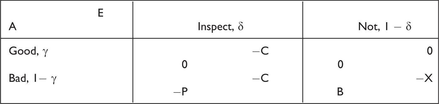
Closer examination of γ* shows that it is decreasing in the externality X and the monitoring cost C, but unaffected by the value of P. Hence, an increase in the absolute sanction has no effect on the athlete’s behavior. It would only induce the enforcer to monitor less frequently (because δ* decreases in P). Punishment has, thus, no marginal deterrence effect. More generally, any player’s equilibrium behavior is independent of his own payoff parameters.

In a model following Becker (1968), the enforcer would be committed to a specific value of δ (and of P, just as in the inspection game). Then, the decision situation of A would not have a simultaneous, but rather a sequential nature: First, society decides on δ and P, then the athlete chooses his behavior. ²⁴ The athlete would be deterred if, and only if, δ and P were fixed such that B < δP. Without any commitment from the enforcer, however, players A and E would be in a simultaneous game and this inequality would govern E’s behavior, as derived previously, rather than the choice of A.

Bayesian Enforcement

Assumptions

Now assume that the athlete and the doping enforcer interact sequentially. After the athlete has made his choice whether or not to use illegal substances, nature produces an informative signal, denoted as i. The signal may assume one out of two realizations: i = g or i = b. The probability of receiving a particular signal realization is contingent on the athlete’s choice: r = Pr(i = g|d = g) and w = Pr(i = g |d = b) with 1 ≥ r ≥ w ≥ 0. ²⁵ The difference between the parameters r and w provides a measure of the enforcer’s monitoring skill:

With r = 1 and w = 0, he monitors perfectly.

With r = w, he has zero monitoring skill.

The intermediate case 0 < w < r < 1 reflects imperfect, but positive monitoring skill.

The enforcer is unable to observe the athlete’s actual choice. He only observes the imperfect signal and updates his beliefs using Bayes’ rule. These ex post beliefs are denoted as µ = Pr(d = g|i = g) and ν = Pr(d = g|i = b). The enforcer has to decide between a sanction (j = s) or an acquittal (j = a). Let α and β represent the enforcer’s behavioral strategies: α = Pr(j = s|i = g) and β = Pr(j = s|i = b).

Just as in the inspection game, the enforcer is assumed to be benevolent, that is, he has an interest in sanctioning correctly. This is included into the model as a payoff G > 0. However, this inability to directly observe the actual behavior of the athlete may occasionally lead to wrongful punishment, which leads to a payoff loss, denoted as –L, with L < ∞. The parameters G and L, thus, reflect the enforcement officer’s interest to issue a sanction if, and only if, the suspect has chosen bad behavior. These payoffs are revealed only after the decision of the enforcer has taken place.

I maintain the assumption P > B from the inspection game: The sanction has to exceed the perpetrator’s benefit from “bad” behavior. Moreover, sanctions are assumed to be inefficient, that is, P > G: The enforcer’s benefit from a justified sanction is smaller than the burden imposed on the athlete. Without this assumption, punishment would generate a welfare gain G – P. This gain might even outweigh the harm from “bad” deeds; under such circumstances, it would even be welfare enhancing to encourage (and then sanction) wrongdoing. All other payoff components are just the same as in the inspection game, which was solved in the previous section.

Figure 2 displays the interaction of the two players and the signals generated in the Bayesian Enforcement Game. The first decision node is in the center of the game tree. Here, the athlete A chooses whether to use doping (d = g) or not (d = b). Then nature chooses the imperfect signal, the realization of which occur with state-dependent probabilities. Enforcer E is unaware of the athlete’s actual choice, but can observe the realization of the signal and, based on this observation, makes his decision to use a sanction or not.

OPEN IN VIEWER

Figure 2.

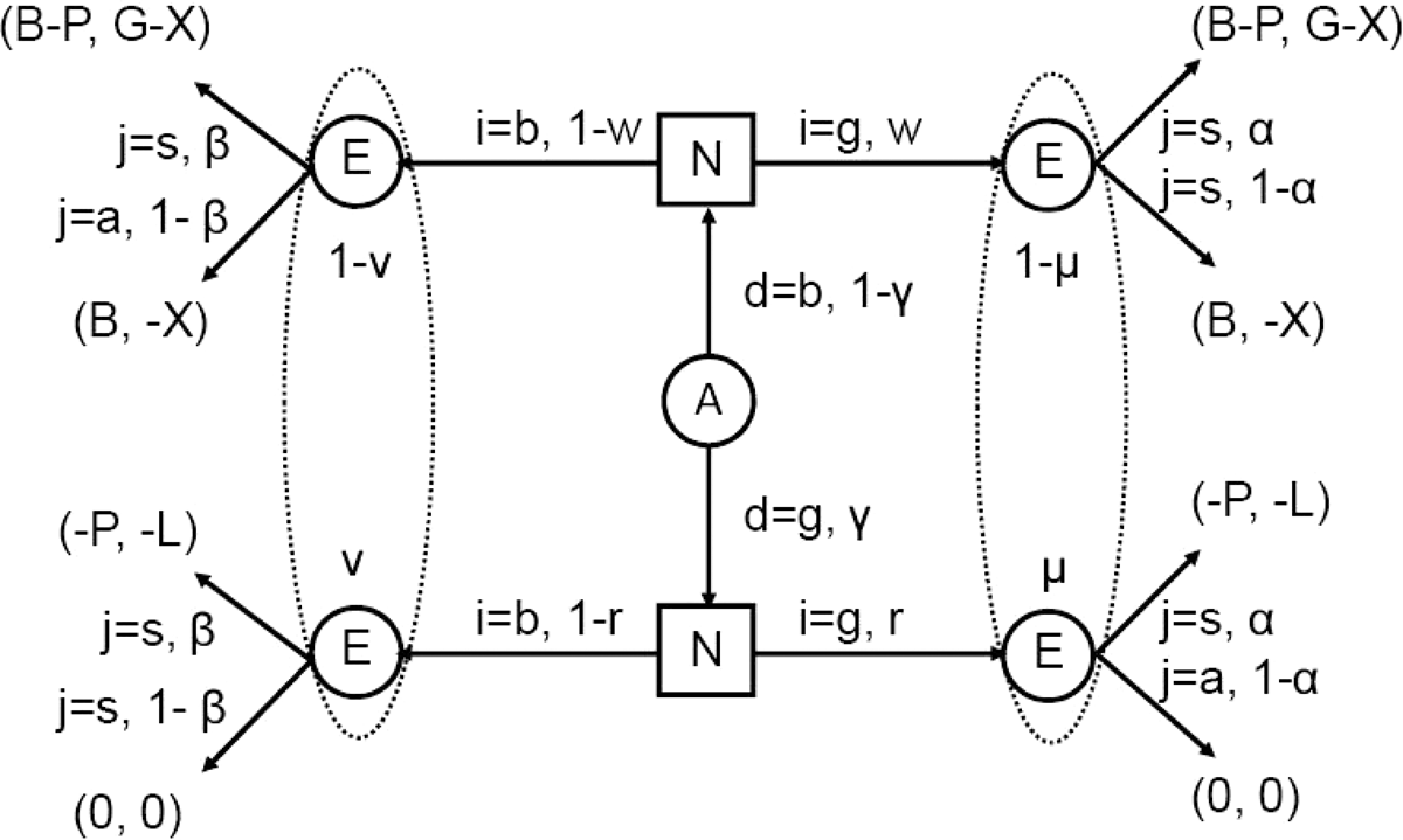
Bayesian enforcement game.

An initial decision of the athlete whether to take part in the contest (or to keep out) could easily be integrated into the model; this is also true for the enforcer’s decision whether or not to use a test should testing be costly. Both players are assumed to be risk-neutral. The payoff parameters (P, B, X, G, L) and the signal quality parameters (r, w) are exogenously given and are common knowledge. Thus, the endogenous variables are α, β, γ, µ, and ν.

The Athlete’s Optimal Choice

The athlete chooses his behavioral strategy γ so as to maximize his expected payoff, given the behavioral strategies (α, β) which he expects the enforcer to play. After each path that ends with j = s, A has to pay a sanction S. If he initially decides for d = b, he receives an additional utility B. Thus, an equilibrium value γ* maximizes

1 − γ B − γ r α + 1 − r β P − 1 − γ w α + 1 − w β P .

1

The first derivative of Equation 1 with respect to γ is P 1 − w β − r − w α − 1 − r β − B . This expression can be simplified to P r − w β − α − B , which leads to the athlete’s BRC γ*(α, β):

γ ∗ = 1 ⇔ β − α > K 0 ≤ γ ∗ ≤ 1 ⇔ β − α = K γ ∗ = 0 ⇔ β − α < K ,

2

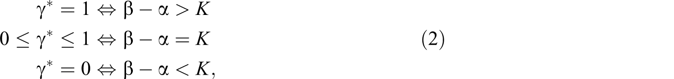
where K is defined as K = B/(r − w)P > 0. ²⁷ The athlete’s BRC immediately implies some intermediate results which will prove useful when deriving the main proposition of this article.

Lemma 1:

If K > 1 ⇔ B > (r – w)P, then (β – α) < K and the athlete is induced to choose γ = 0.

If K = 1 then β – α ≤ K. The enforcer’s choice of β = 1 and α = 0 is the only strategy that makes the athlete choose a γ with 0 < γ < 1.

K < 1 is a necessary (albeit not sufficient) condition for β – α < K which would induce the athlete to choose γ > 0.

If γ* = 0 or γ* = 1, then the athlete chooses a pure strategy, while 0 < γ* < 1 represents the choice of a mixed strategy. Figure 3 illustrates the athlete’s BRC γ* = γ*(α, β) for parameter settings with K < 1:

The bold pentagon in the lower-left corner of the figure includes the (α, β) combinations to which the athlete’s optimal reaction is γ = 0.

The bold triangle in the upper-right corner is situated above the (α, β) combinations that induce the athlete to choose γ = 1.

Finally, the bottom line of the bold square in the center of the figure describes the (α, β) combinations that keep the athlete indifferent between all of his mixed strategies.

OPEN IN VIEWER

Figure 3.

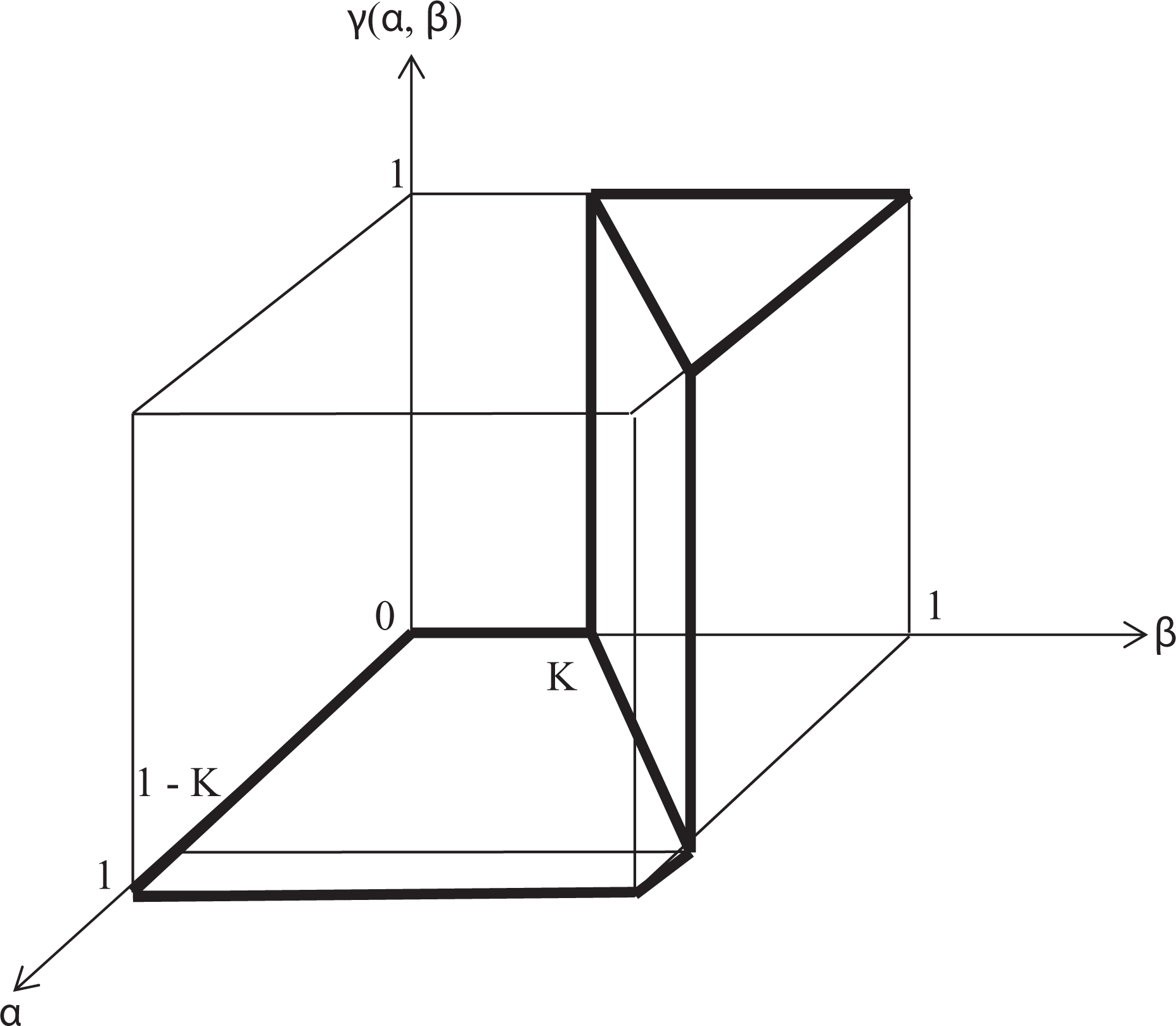
Athlete’s best response correspondence γ* (α, β) for K < 1.

With K = 1, which is equivalent to B = (r – w)P, the bold square is located at α = 0 and β = 1. Hence, the upper triangle would shrink to zero. In such a parameter setting, the athlete’s BRC reduces to γ* ∊ [0, 1] for α = 0, β = 1, and γ* = 0 otherwise.

Optimal Choice of the Doping Enforcer

A rational doping enforcer chooses his action, given his anticipation of the behavioral strategy chosen by the athlete. From a strategic point of view, the game resembles a simultaneous one, because no player can directly observe the respective other player’s choice when making their own decision. However, the enforcer observes an imperfect signal triggered by the athlete’s actual behavior (which requires a sequential time structure) and, thus, he can make a decision contingent on the realization of this signal.

First, I examine the enforcer’s optimal choice after having observed the signal realization i = g. In this case, Bayesian updating leads to the following ex post belief:

μ = r γ r γ + w ( 1 − γ ) .

3

Taking these ex post beliefs into account, the enforcer chooses his behavioral strategy α* so as to maximize [(1 − µ) (αG – X) – µαL]. The first derivative of this with respect to α is given by G – µ(G + L). ²⁸ The relation between the optimal α and the athlete’s strategy choice γ becomes clear if Equation 3 is used to substitute μ. Then, the first derivative can be rewritten as

G − r γ r γ + w ( 1 − γ ) ( G + L ) .

This is negative if, and only if, ²⁹

γ > w G r L + w G = γ 1 .

For later use, the right-hand side of this inequality is denoted as γ₁. The relation between the athlete’s choice γ and the behavioral strategy of the enforcer after having observed i = g is summarized in the following BRC α* = α*(γ)

a ∗ = 1 ⇔ γ < γ 1 0 ≤ a ∗ ≤ 1 ⇔ γ = γ 1 a ∗ = 0 ⇔ γ > γ 1 ,

4

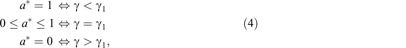
given w > 0. In the same vein, the optimal behavior strategy β*(γ) can be derived for the case in which the enforcer has observed the signal realization i = b. Bayesian updating induces the ex post belief

ν = ( 1 − r ) γ ( 1 − r ) γ + ( 1 − ω ) ( 1 − γ ) ,

5

and the enforcer chooses β so as to maximize [(1 – ν)(βG – X) – νβL]. The first derivative with respect to β is G – ν(G + L). Substitution of ν allows to state the BRC β* = β*(γ) as

β ∗ = 1 ⇔ γ < γ 2 0 ≤ β ∗ ≤ 1 ⇔ γ = γ 2 β ∗ = 0 ⇔ γ > γ 2 ,

6

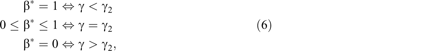
with γ 2 = ( 1 − w ) G ( 1 − r ) L + ( 1 − w ) G . The enforcer’s BRC immediately implies some useful results that are listed in Lemma 2.

Lemma 2:

0 < w < r < 1 ∧ G > 0 ∧ L < ∞ implies 0 < γ₁ < γ₂ < 1.

If w = 0, then α* = 0 and γ₁ = 0.

r = 1 implies β* = 1, γ₂ = 1, µ = 1, and ν = 0.

Figure 4 displays the signal-contingent BRC of the enforcer for the case of γ₁ > 0 and γ₂ < 1. The BRC α*(γ) is represented by the dashed line, whereas the straight line represents β*(γ). The figure demonstrates that there is no value of γ for which α*(γ) > β*(γ). Therefore, the equilibrium analysis can be limited to enforcer’s strategies with α ≤ β.

OPEN IN VIEWER

Figure 4.

BRC α*(γ) and β*(γ) of the enforcer.

Equilibrium Analysis

In the previous section, I have derived the BRCs α* = α*(γ) and β* = β*(γ) of the enforcer, as well as the athlete’s BRC γ* = γ*(α, β). An equilibrium combination of behavioral strategies is given by α*(γ*), β(γ*), and γ*(α*, β*). The following terminology characterizes the different possible types of equilibria. An equilibrium is called

tyrannic if the enforcer sanctions with certainty (α = 1);

draconian if he punishes with positive probability (1 > α > 0);

lenient if he abstains from issuing a sanction (α = 0)

after having observed the “good” signal realization. The following proposition presents the (behavioral) strategy combinations that characterize the PBE of the game (the proof has been confined to Appendix A). Recall that

K = B ( r − w ) P > 0 , γ 1 = w G r L + w G > 0 , a n d γ 2 = ( 1 − w ) G ( 1 − r ) L + ( 1 − w ) G .

7

Proposition 1: The Bayesian Enforcement game with G, L > 0, L < ∞, and 0 < w < r < 1 has the following PBE {(α*, β*); (μ*, ν*); γ*}:

If K < 1, then the game has three types of PBE:

tyrannic: {(1, 1); (0, 0); 0};

draconian: {(1 – K, 1); (µ*, ν*); γ₁} with µ* = rγ₁/[w + (r – w)γ₁] and ν* = (1 – r)γ₁/[1 – w – (r – w)γ₂];

lenient: {(0, K); (µ*, ν*); γ₂} with µ* = rγ₁/[w + (r – w)γ₂] and ν* = (1 – r)γ₁/[1 – w – (r –w)γ₂].

If K = 1, then the game has two types of PBE

a tyrannic one: {(1, 1); (0, 0); 0};

the set {(0, 1); (0, 1); γ*} with γ* ∊ [γ ₁, γ ₂] contains limit cases of the lenient equilibrium.

If K > 1, then only a tyrannic equilibrium {(1, 1); (0, 1); 0} exists.

The tyrannic equilibrium is the only type in which pure strategies are chosen. It can occur in all three of the parameter settings: K > 1, K = 1, and K < 1. In such an equilibrium, the athlete will choose doping with certainty. The draconian equilibrium is characterized by a positive rate of compliant (good) behavior. While the athlete faces a positive probability of being sanctioned after both signal realizations, he can influence this probability by his own choice.

In the lenient equilibrium, the threat of sanctions is rather moderate (only after the bad signal realizations, and then with a probability smaller than 1), and good behavior occurs with the highest probability. If the parameters B, P, r, w are calibrated such that K = 1, the lenient equilibria are characterized by a certain punishment after having observed the bad signal realization, and no punishment after the good one. However, there are multiple equilibria of this type, as any compliance probability between γ₁ > 0 and γ₂ < 1 can be carried out by the athlete.

The highest compliance rate (namely γ₂) is obviously obtained in the case K < 1 if the parties coordinate on the lenient equilibrium. In this equilibrium, no sanction is carried out after the good signal realization, and the probability of a sanction is smaller than one (namely K) if the signal realization indicates doping. Figure 5 displays the three equilibria (for the case K < 1) as bold dots.

OPEN IN VIEWER

Figure 5.

Bayesian enforcement: equilibria.

The first result (1a) is rather straightforward: If the athlete chooses bad behavior, and the enforcer punishes regardless of the signal realization, both parties’ beliefs will be confirmed by the respective other party’s behavior. In this equilibrium, the ex post beliefs of the enforcer are µ = ν = 0. This is one important difference to the inspection game, in which no pure strategy equilibrium exists.

Result (1b) has a rather counterintuitive property. The enforcer can induce the athlete to choose good behavior with probability γ₁ if he always punishes him after having observed the bad signal realization (β* = 1), and he also punishes with a positive probability after having observed the good signal realization (α* > 0). However, the resulting equilibrium probability of good behavior is lower than in the lenient equilibrium.

The lenient equilibrium (1c) establishes that it can be rational for an athlete to frequently choose good behavior under costless monitoring if the enforcer never punishes after having observed i = g and only occasionally after i = b. In the lenient equilibrium, E’s ex post beliefs are

μ = r γ 2 r γ 2 + w ( 1 − γ 2 ) = r ( 1 − w ) G r ( 1 − w ) G + w ( 1 − r ) L ,

and

ν = ( 1 − r ) γ 2 ( 1 − r ) γ 2 + ( 1 − w ) ( 1 − γ 2 ) = ( 1 − r ) ( 1 − w ) G ( 1 − r ) ( 1 − w ) G + ( 1 − w ) ( 1 − r ) L = G L + G .

The equilibrium belief ν is independent of (r, w), as the equilibrium choice of β neutralizes the signal’s imperfection. In both mixed-strategy equilibria, the monitor is required to choose β > α. If the distance between these two signal-contingent punishment probabilities is calibrated adequately by the enforcer’s strategy choice, then the athlete is indifferent between his pure strategies. This effect can either be attained by choosing α = 0 and an adequately high β < 1, or by choosing β = 1 and an adequately low α > 0. Then the monitor’s ex post beliefs in the draconian equilibrium are

μ = r γ 1 r γ 1 + w ( 1 − γ 1 ) = r w G r w G + r w L = G G + L ,

and

ν = ( 1 − r ) γ 1 ( 1 − r ) γ 1 + ( 1 − w ) ( 1 − γ 1 ) = ( 1 − r ) w G ( 1 − r ) w G + ( 1 − w ) r L .

Now, it is the equilibrium choice of α that makes the ex post belief µ independent of the signal quality. If a game exhibits multiple equilibria, using it as a positive tool would require criteria for equilibrium selection. However, it is beyond the scope of this article to discuss this question in more detail. ³⁰ The impossibility of implementing good behavior with certainty, even in a world with zero testing cost, is directly implied by Proposition 1. Moreover, Proposition 1 also directly implies that the enforcer’s strategy to sanction if, and only if, the test signal is “bad” can be part of a Bayesian equilibrium. Both results contribute to the main insights derived in this article.

Corollary: In the Bayesian enforcement game with G > 0, L > 0, and 0 < w < r < 1:

The athlete’s strategy γ = 1 is never part of a perfect Bayesian equilibrium;

α = 0 and β = 1 is the enforcer’s equilibrium strategy in both the draconian and the lenient equilibrium if, and only if, K = 1.

With K ≠ 1, E’s strategy α = 0, β = 1 is never part of a perfect Bayesian equilibrium.

Proof: Parts 1 and 3 of this corollary can directly be seen in Proposition 1. Part 2 can be inferred from the athlete’s BRC and claim no. 2 of Lemma 1. If the enforcer, with K = 1, does not choose (α, β) = (0, 1), then A’s best reply is γ = 0, to which the enforcer would reply α = β = 1 . If, however, E chooses α = 0 and β = 1, this would make A indifferent between his pure strategies. If A chooses γ = γ₁, then the two players are in a limit case of the draconian equilibrium in which β = 1 and α = 1 – K = 0 (due to K = 1). If A happens to choose γ = γ₂, then they are in a limit case of the lenient equilibrium with α = 0 and β = K = 1 (due to K = 1).

This result formalizes what has been discussed verbally in the introduction. At first glance, it seems to be desirable for the enforcer to carry out an enforcement strategy that punishes with certainty if, and only if, he receives the “bad” signal, that is, to choose α = 0 and β = 1. However, this is not part of an equilibrium if K ≠ 1. K > 1 leads to the tyrannic equilibrium, and if K < 1, then this enforcement strategy induces the athlete to choose γ = 1, to which the best reply of the benevolent enforcer would be α = β = 0. The only way to avoid being misled by the imperfect signal realization is to neglect it, if the enforcer expects the athlete to comply anyway. Following the signal realization, on the other hand, would bear the risk of rendering unjust punishment (with probability w). The only exception is the case of K = 1, which is equivalent to B = P(r – w). If society sets the parameter B, P, r, and w this way, then the enforcer would induce the athlete to choose some γ between γ₁ and γ₂ by setting his punishment strategy to α = 0 and β = 1 (which implies β – α = K as K = 1).

Discussion

Comparative Statics of the Lenient Equilibrium

The equilibrium analysis reveals that the enforcer’s behavior does not depend on his own payoff parameters. The only parameters that influence his behavioral strategies in the equilibria are B, P, r, and w. In the lenient equilibrium, the probability of punishment after having observed the bad signal realization (i = b) is β* = K (after the good signal realization, the enforcer will never punish: α = 0). Remember that K = B/[(r – w)P]. Comparative static analysis shows that

∂ β ∗ ∂ B , ∂ β ∗ ∂ w > 0 > ∂ β ∗ ∂ P , ∂ β ∗ ∂ r .

Thus, a better signal quality (i.e., a higher r or a lower w), a lower athlete’s benefit B, or a higher sanction P would decrease the probability of punishment after the enforcer has observed the bad signal realization in the lenient equilibrium. The athlete chooses good behavior with probability γ₂, which depends on r, w, L, and G. The signs of the partial derivatives are

∂ γ 2 ∂ G , ∂ γ 2 ∂ r > 0 > ∂ γ 2 ∂ L , ∂ γ 2 ∂ w

The probability of good behavior can be increased by increasing the enforcer’s reward for the correct decisions, by lowering his disutility from wrong decisions, or by increasing the signal quality. In the context of doping, this result implies that a higher test quality would induce the athlete to comply with higher probability, whereas the enforcers would mete out the punishment with a lower probability. These intuitive results, however, are limited to the lenient equilibrium.

Comparative Statics of the Draconian Equilibrium

The comparative statics of the results of the draconian equilibrium are different. Here, the enforcer chooses a mixed punishment strategy α* = 1 – K after having observed the good signal realization (and punishes with β = 1 after having observed the bad realization). The signs of the partial derivatives are

∂ α ∗ ∂ B , ∂ α ∗ ∂ w < 0 < ∂ α ∗ ∂ P , ∂ α ∗ ∂ r .

The athlete chooses good behavior with a probability of γ₁. Again, this probability only depends on r, w, L, and G. The signs of the partial derivatives are

∂ γ 1 ∂ G , ∂ γ 1 ∂ w > 0 > ∂ γ 1 ∂ L , ∂ γ 1 ∂ r .

In the draconian equilibrium, a higher signal quality, that is, dr > 0 > dw, would increase the probability of wrongful punishment α*, which is rather counterintuitive. Moreover, higher signal quality would decrease the probability of good behavior γ₁ in this equilibrium. A benevolent enforcer, however, would prefer the athlete to choose a higher value of γ.

Conclusion

The Bayesian enforcement model, based on the assumption of imperfect doping tests, leads to results that differ from those of the enforcement models in the tradition of Becker (1968) or of the inspection game:

Whereas in a simple Becker model the enforcer would either produce perfect deterrence or no deterrence at all, in the Bayesian enforcement game total deterrence is never part of a perfect Bayesian equilibrium.

One policy implication of these results would be for sports associations to employ means that foster the selection of the lenient equilibrium. ³¹ In the lenient equilibrium, an investment in higher signal quality would improve athletes’ compliance. In the draconian equilibrium, however, such an investment would be even counterproductive.

It is remarkable that in none of the possible equilibria the athlete chooses compliant (good) behavior with certainty, as long as the monitoring signal is imperfect. This result holds despite the assumption that the enforcer has undistorted incentives and the doping test is costless. A rational enforcer should not base his decision on such an imperfect signal if he believes the athlete to choose good behavior. In that case, Bayesian updating induces the enforcer not to punish the athlete, even if the signal realization is “bad.” That would, however, invite the athlete to choose “bad” behavior.

The enforcer might consider a strategy according to which he issues a punishment if, and only if, the test result indicates the usage of illicit drugs, but never if the realization of the test signal is “good,” that is, to choose α = 0 and β = 1. However, this policy is an equilibrium strategy in the Bayesian enforcement game only in an exceptional case: If society has chosen the parameter P according to the value of B, r, and w such that K = 1. The athlete would then be indifferent between his pure strategies.

Choosing either γ₁ or γ₂ would lead to a perfect Bayesian equilibrium. The first one leads to a limit case of the draconian equilibrium type, whereas the second is a special case of the lenient equilibrium type. Hence setting the policy parameter P, r, and w (in combination with the value of B) such that K = 1 is not welfare optimal, as it leaves open which compliance rate will be played. A compliance rate of γ₂ can only be reached by setting K < 1 and inducing the enforcer to choose α = 0.