Constitutional Change and American Pivotal Politics

Abstract

Recent studies of legislative gridlock espouse the importance of institutional design in separation-of-powers games. However, few scholars have focused on the effects of the adoption of the U.S. Constitution on legislative gridlock. This article attempts to fill that gap by determining whether the Constitution improved the marginal effect of the gridlock interval on the ability to change policy. Results suggest that policy is more responsive to the range of pivotal players (in both the negative and the positive direction) under the Constitution than under the Articles of Confederation, providing empirical evidence that it may be the superior design.

Keywords

Constitution Articles of Confederation gridlock legislation

It has been said that legislative “gridlock” is as much an American tradition as apple pie (Brady & Volden, 2006). If that is the case, calls for legislative reform and constitutional amendment are equally iconic elements of Americana. Current calls to modify the filibuster in the U.S. Senate (Mondale, 2011), to expand the size of the U.S. House (Baker, 2009), and to allow states the power to nullify federal legislation (Zernike, 2010) would significantly affect legislative gridlock if they were enacted. According to those who advocate such reforms, changing these institutions should produce better policies.

Despite repeated claims that gridlock is the result of institutions, very little is understood about the most radical institutional change in U.S. history—the transition from the Articles of Confederation to the Constitution—and how it affected gridlock. Most, although not all, perceive this transition as a somewhat ambiguous success in creating a more “positive” or “proactive” national government that could pass more laws. However, these claims are largely descriptive and anecdotal (Brown, 1993; Holcombe, 1991; Jensen, 1965). Empirical evaluations of the transition, such as Aldrich et al. ( Aldrich et al. (2002), are rare.

In this article we show that the Constitution not only decreased legislative gridlock, thereby allowing more legislation to pass, it also made policy more responsive to the gridlock interval.¹ Meaning, if we took identical sets of political actors and place them in the two different institutional configurations, the legislative outcomes produced by the Constitution would be more reflective of the range of preferences between the pivotal actors² than the legislative outcomes produced by the Articles of Confederation. This goes a step further than the traditional argument that bloc voting, supermajority requirements, and other institutions curbed legislation under the Articles of Confederation (Aldrich et al., 2002). Bicameralism and the introduction of a presidential veto player make it unclear whether the Constitution or the Articles of Confederation increased legislative output. Hence, that question has not been fully resolved. In going a step further, we show that the gridlock interval had a limited effect under the Articles of Confederation. Few bills passed and expenditures barely changed, almost regardless of the gridlock interval. In contrast, the Constitution constrained government when pivotal actors were far apart and enabled government when pivotal actors were close together. In this sense, the Constitution provided a design that was more responsive to pivotal actors, consistent with Madison’s arguments for a strong government with checks and balances (Federalist 51).

Why should scholars care about the primary, if not only, constitutional transition in U.S. history? From a uniquely American perspective, scholars should want to know whether the Constitution is more or less responsive to changes in preferences than other institutional designs. This is especially true for those who claim the Constitution itself is responsible for particular legislative successes or failures. From an international perspective, modern constitutional reformers should want to know which constitutions facilitate government action and which promote policy stability. Regardless of whether readers desire a more proactive government or more constrained one, the performance of institutions should be a concern for any present-day institutional architect, particularly those who want to compare presidential systems to confederative designs more broadly. Our study is a first step in that direction.

We proceed in two stages. First, we determine whether the Constitution significantly affected the nation’s ability to change policy between 1777 and 1829 given a number of controls. For this analysis we measure the ability to change policy using the volume of enacted legislation and the change of government expenditures in separate regressions. Second, we examine whether the marginal effect of the gridlock interval differed between the Articles of Confederation and the Constitution. In other words, we determine whether a gridlock interval of comparable length had the same effect under the two documents. This helps us determine whether one set of institutions is more responsive to the relative preferences of pivotal actors than the other, and if so, which one.

We find that the Constitution decreased the average gridlock interval, increased the volume of legislation, and facilitated the ability to change government expenditures. More important, we discover that the Constitution improved the marginal effect of the gridlock interval on the ability to change policy. By examining an interaction between the gridlock interval and a dummy variable for enactment of the Constitution, we find that the gridlock interval had a greater marginal effect on the volume of statutes, and change in government expenditures, under the Constitution than under the Articles of Confederation. This demonstrates that legislation was more responsive to legislative institutions under the Constitution (in both a positive and a negative direction) and that the Constitution arguably outlines the more effective form of government. We conclude that the historic growth of the U.S. government, although not entirely attributable to the Constitution, was made more reflective of legislative demand by the Constitution.

A Tale of Two Governments

The Articles of Confederation organized the United States into a confederation of 13 sovereign states. Although they were not officially ratified until 1781, the Articles served as the de facto national government as soon as they were proposed by Congress in 1777. They governed federal institutions until 1789 when the Constitution was enacted.

Under the Articles of Confederation, each state legislature annually elected two to seven delegates to represent their state in Congress (Article V). Every state determined the exact size of its delegation within this range. Delegates could be recalled, occasionally fell too ill to serve, or died while in office. As a result, appointments were generally more frequent than annual. Of the 437 delegates elected between 1774 and 1789, 92 of them (21%) never served. Many more arrived late or departed before their term expired.

The unicameral Congress of the Confederation ran the legislative, executive, and bare judicial functions of the national government. All floor decisions were made using a forward agenda³ with votes taken in state blocs. Rather than making use of a powerful rules committee, the agenda was completely decentralized. Any delegate could make a proposal at any given time. After a bill or amendment was debated, each state vote was determined by the absolute majority of their delegation. If a state delegation was numerically split on an issue, the state was counted as divided. State votes were then tallied and the proposal would pass if the yeas exceeded seven states (a majority of the confederation) or nine states (a supermajority), depending on the type of legislation at hand.

Legislation was split into two types, each with a unique voting threshold. Major issues required the approval of 9 of the 13 states and covered decisions to engage in war; grant letters of marque or reprisal; enter treaties or alliances; borrow, appropriate, or coin money, or regulate the value thereof; ascertain expenses; emit bills of credit; agree upon the number of naval vessels, land forces, or sea forces to be raised; and appoint a commander in chief of the armed forces (Article IX). All other issues were considered minor and required the approval of seven states. To name a few, minor issues included administrative tasks like paying military officers, managing military logistics, regulating post offices, and issuing instructions to ambassadors.

Although there was a president of Congress, the post was primarily ceremonial. The President could not veto or direct debates, similar to the functions of the President Pro Tempore in the current Senate. There was no formal executive or judicial branch of the government and no need for presidential approval of legislation. With the exception of major issues, the institutions that governed minor issues under the Articles of Confederation were essentially majoritarian in nature.

When operations began on March 4, 1789, the Constitution moved the nation away from majoritarianism and toward institutions based on a separation of powers. As we know, the Constitution established a judicial branch, an executive with veto power, and two legislative chambers with differing electoral criteria. Alone such changes should increase the gridlock interval for minor issues and constrain legislation. However, the Constitution also tallied votes among members individually, rather than tallying votes in state blocs, and it eliminated the distinction between minor and major issues. The Constitution also changed governmental power in ways that could potentially change policy without changing the length of the gridlock interval.⁴ Although we recognize that such powers could account for differences in the ability to change policies under the two constitutions, it is impossible to isolate the effects of specific powers and institutional changes that occur simultaneously. Hence, we can show that the Constitution decreased the gridlock interval and made policy more responsive to the preferences of legislative actors, but we cannot say this is solely due to changes in the legislative process.

Notes on the Theoretical Model

Like Krehbiel (1998), Brady and Volden (2006), and Chiou and Rothenberg (2003, 2008), we assume a single-dimensional policy space and actors with single-peaked and symmetric utility. We also assume that status quo points are uniformly distributed across the dimension. Under the Articles of Confederation, for minor legislation, critical players include the median member of the seventh state from the right to the median member of the seventh state from the left. All points within this range are in equilibrium. If 13 states attended and the median delegation had an odd number of members, then this range would be a single point. If fewer than 13 states attended, the median delegation had an even number of members, or there were an even number of delegations on the floor, then the set of equilibrium points would be a range. The latter was always the case for our data. For major legislation, the points ranging from the median member(s) of the ninth state from the right to the median member of the ninth state from the left are in equilibrium. Under the Constitution, critical players include the median voters of the House and the Senate, the two-thirds override pivots, and the President. Key differences between our model and the models presented by earlier scholars is that we do not include the filibuster pivot,⁵ we do not assume that a single actor is the proposer,⁶ and we do not model the effect of political parties in our primary results.⁷ These institutions are all consistent with the Constitution’s initial design.

Empirical Specification

We measure the ability to change policy using two different variables. The first is the number of statutes enacted, similar to the measure used by Krehbiel (1998), Brady and Volden (2006), and Chiou and Rothenberg (2003, 2008).⁸ The theory behind this regression is that each statute enacted creates a change in policy.

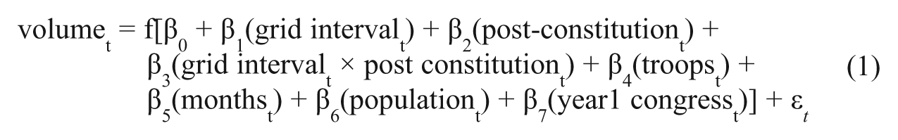
{volume}_{t} = f [β_{0} + β_{1} ({grid interval}_{t}) + β_{2} ({post-constitution}_{t}) + β_{3} ({grid interval}_{t} \times {post constitution}_{t}) + β_{4} ({troops}_{t}) + β_{5} ({months}_{t}) + β_{6} ({population}_{t}) + β_{7} ({year1 congress}_{t})] + ε_{t}

where the βs are the parameters to be estimated, t is the year (post-Constitution congresses are annualized), and ϵ_t is a random error term.

Our data begin in 1777 because the first roll-call votes were recorded that year. We end our study after the 20th Congress (1829) because legislation became increasingly intertwined with political parties during the second-party system (Aldrich, 1995, p. 99; McCormick, 1966, p. 335). This allows for a total of 52 observations, 12 of which are prior to the Constitution.⁹

In this specification, volume _t is the number of statutes enacted in year t. This includes acts that passed Congress under the Articles of Confederation (1777-1788) and acts that passed both Congress and the President, or the two-thirds override, under the Constitution (1789-1829). To make the data comparable, statutes were divided into major and minor issues based on policy type for both the Articles of Confederation and the Constitution. Categories for major and minor legislation were derived from Article IX of the Articles of Confederation. The type of each roll call was determined from Lord’s (1984) codebook for the Congress of the Confederation and from the United States Statutes at Large (1854) for the post-Constitution era. The two types are analyzed in separate regressions.

Grid interval is the length of the gridlock interval. It measures the relative length of points in sub-game perfect equilibrium (the theoretical prediction of the degree of gridlock) given the procedural rules and the estimated ideal points of those who held office during period t. Larger intervals are associated with greater gridlock with a feasible range between 0 and 2. Under the Articles of Confederation, gridlock intervals were calculated as the average annual gridlock interval for each month Congress attempted to be in session. In cases where Congress attempted to meet but attendance records indicate they had less than the required number of states to pass legislation, we treat the month as having the maximum gridlock interval of two. This reflects the fact that all points in the policy space are in equilibrium and cannot be overturned without more states in attendance. As a robustness check, we conducted a parallel analysis that excluded months where the legislature failed to make quorum rather than coding them as 2s. This did not affect our substantive results.¹⁰ A detailed description of the construction of the gridlock interval, and other data sources, are described in the appendix.

The second independent variable, post-Constitution, is a dummy variable indicating whether the congressional year was before (= 0) or after (= 1) the enactment of the Constitution. If the Constitution was a more enabling document than the Articles of Confederation, as many historians and political scientists have claimed (Aldrich et al., 2002; Jillson & Wilson, 1994), then we would expect β₂ > 0.

Our third independent variable is an interaction term that determines whether the gridlock interval had differing effects on the two constitutions. Because post-Constitution is a dummy variable, the parameter β₁ by itself represents the effect of the gridlock interval under the Articles of Confederation. The effect of the gridlock interval under the Constitution is represented by β₁ + β₃. If the Constitution increased the effect of gridlock intervals on the volume of legislation, then we would expect β₁ + β₃ < β₁ < 0. Effectively, smaller gridlock intervals would be associated with more statutes under the Constitution than comparable sizes would be under the Articles of Confederation.

Our remaining independent variables are a series of controls. Troops is the total number of U.S. soldiers in active duty, scaled in thousands. We include it to control for external and internal threats indirectly. Measuring threats using domestic troop levels, rather than foreign troop levels, allows us to control for the intent of foreign nations, alliance structures, the deployment of foreign troops, and domestic security concerns such as Native American uprisings. In equilibrium, domestic troop levels should adjust to these nuances if the demand for defense does not exceed capacity (Garfinkel & Skaperdas, 2007). Because Congress micromanaged the military during both periods, we hypothesize that β₄ > 0.

Months indicates the total number of months that Congress attempted to be in session each year. We include this variable to control for periods where Congress could not pass legislation because it was not in session. Any month where Congress attempted to meet for at least 5 days is counted as a session month. This includes cases where an insufficient number of states attended to conduct business. We hypothesize that β₅ > 0.

Population measures the total U.S. population, including territories, in millions (Coulson & Joyce, 2003). We include it to capture increased demands for legislation as the size of the nation increases. We hypothesize that β₆ > 0.

Finally, year1 Congress is a dummy variable that equals 1 for the first year of a post-Constitution Congress, zero otherwise. As we will see, under the Constitution more statutes were enacted in the second year of a Congress than in the first due to a legislative cycle of marking up bills in the first year and passing them in the second. Including this variable accounts for the legislative cycle. Descriptive statistics for each variable are listed in Table 1.

Table 1.

Data Summary

	Mean	SD	Min.	Max.
Number of statutes (minor)	29.269	30.929	0.000	97.000
Number of statutes (major)	16.846	16.429	0.000	58.000
Gridlock interval (minor)	0.327	0.233	0.099	1.265
Gridlock interval (major)	0.420	0.368	0.099	1.512
Post-Constitution (dummy)	0.769	0.425	0.000	1.000
Troops (in thousands)	11.950	11.196	0.700	46.858
Session months	6.372	3.217	2.800	12.000
Population (in millions)	6.651	2.785	2.793	12.434
Government expenditures (in millions)	12.237	8.234	0.579	29.495
GDP (in millions)	635	328	183	1,366
Year 1 Congress (dummy)	0.385	0.491	0.000	1.000
Positive (dummy)	0.509	0.506	0.000	1.000

Note: For all variables, N = 52. Expenditures and GDP are reported in millions of 1800 dollars.

The Effect of the Gridlock Interval on Government Expenditures

Another potential measure of the ability to change policy is government expenditures. Recognizing that fiscal policy expands and contracts by increasing and decreasing expenditures leads to our second specification.

\begin{array}{l} ({expend}_{t} - {expend}_{t - 1}) = α_{0} + α_{1} ({grid interval}_{t} - {grid interval}_{t - 1}) + α_{2} ({post-constitution}_{t}) + α_{3} ({grid interval}_{t} - {grid interval}_{t - 1}) \\ \times {post-constitution}_{t}) + α_{4} ({troops}_{t} - {troops}_{t - 1}) + α_{5} ({months}_{t} - {months}_{t - 1}) + α_{6} ({GDP}_{t} - {GDP}_{t - 1}) + α_{7} ({year1 congress}_{t}) + α_{8} ({positive}_{t}) + ε_{t} \end{array}

where the α′s are parameters to be estimated, and ϵ_t is a random error term.¹¹ In specification (2) we assume that expenditures revert to zero each year unless a continuing resolution is passed.¹² This suggests that each expenditure reflects a unit of fiscal policy rather than a change of policy as is the case of the number of statutes. As such, first differences are appropriate.¹³ With the exception of the first differences, grid interval, post-Constitution, troops, months, and year1 Congress are the same variables as stated previously. We expect the same signs as before.

The gross domestic product (GDP) is used instead of population because change in GDP is a better measure of the nation’s ability to increase government expenditures than changes in population. If resources are insufficient and borrowing infeasible, government expenditures cannot expand, regardless of increases in population or any other sort of internal demands. Because government expenditures typically increase with an expanded economy, we hypothesize that α₆ > 0.

Positive is a dummy variable indicating whether government expenditures increased (= 1) from the previous year. We include it to capture differences in the legislative process for increasing and for decreasing government expenditures.¹⁴ We hypothesize that α₈ > 0.

Specification issues

Because specification (1) includes a count variable as the dependent variable, least squares estimates might be inefficient, inconsistent, and biased (Long, 1997). We considered Poisson regression because of the count data. However, likelihood ratio tests indicate that a Poisson regression is weakly overdispersed (for both major and minor statutes). Hence, we report estimates for specification (1) using negative binomial regression. Poisson regression produced similar results.

None of our models showed signs of first-order autocorrelation.¹⁵ Because changes in constitutional design can affect the standard error of the disturbance term, we estimated all regressions using Huber–White robust standard errors to account for potential heteroskedasticity.

Results

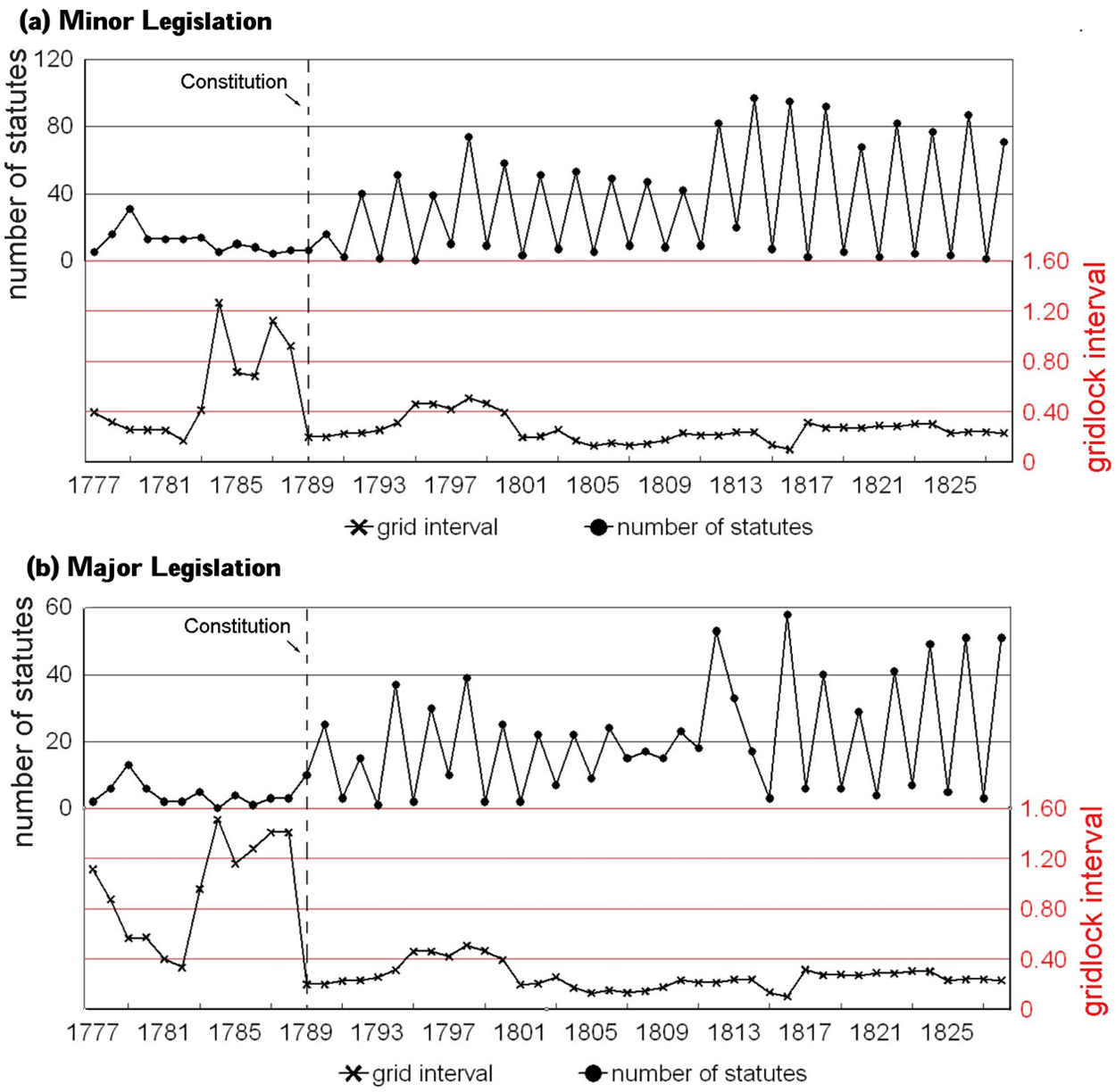
Figure 1 shows the number of minor statutes and major statutes for each period in the top part of the graph and the associated gridlock interval in the bottom part of the graph. The first thing to notice is the dramatic increase in enactments in the second year of a post-Constitution Congress. This variation is accounted for using the year1 Congress dummy.

Figure 1.

Volume of statutes

The next thing to notice is that the average volume of statutes (both major and minor) increased with the adoption of the Constitution from 11.5 minor statutes under the Articles of Confederation to 34.6 under the Constitution. Similarly, the average number of major statutes increased from 3.9 under the Articles of Confederation to 20.7 under the Constitution. Difference of means tests suggests that both differences are significant at the .01 level.

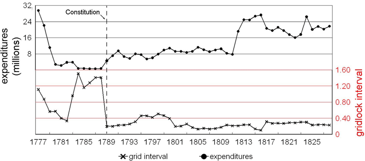
The same comparison can be made for government expenditures (see Figure 2). Average government expenditures were US$6.5 million under the Articles of Confederation and US$13.9 million under the Constitution (significantly different at the .01 level). Perhaps more important, the change in government expenditures increased from an average of −1.570 under the Articles of Confederation to an average of 0.525 under the Constitution. This difference just misses the .05 level of significance (p = .052).

Figure 2.

Government expenditures

At the same time, the average gridlock interval was larger under the Articles of Confederation than it was under the Constitution. For minor issues, the average gridlock interval was 0.563 under the Articles and 0.256 under the Constitution. Similarly, for major issues, the average gridlock interval was 0.965 under the Articles and 0.256 under the Constitution. A difference of means tests suggest that the pre- and post-differences for both minor and major issues were significant.

This suggests that the volume of statutes and the size of government expenditures were larger when the gridlock interval was smaller. However, it does not show that these variables are related by year. Evaluating such a relationship requires an analysis similar to the one outlined in specifications (1) and (2).

The Constitution’s Effect on the Volume of Statutes

Because the constitutional components of the gridlock interval (such as institutional rules) cannot be separated from the nonconstitutional components (such as the preferences of politicians), we first exclude the gridlock interval from our regressions to help isolate the effect of the Constitution on the volume of legislation passed, as shown in Columns A and B, Table 2. The table reports coefficient estimates for determinants of the volume of statutes. Each coefficient has the hypothesized sign.

Table 2.

Determinants of the Volume of Statutes

	(A) Minor laws	(B) Major laws	(C) Minor laws	(D) Major laws
Gridlock interval			−0.706* (0.316)	−0.420 (0.707)
Post-Constitution	2.493** (0.330)	3.296** (0.465)	1.991** (0.538)	3.091** (1.107)
Gridlock × Post-Construction			0.720 (0.751)	−0.324 (1.021)
Troops	0.024** (0.007)	0.020 (0.016)	0.019** (0.007)	0.016 (0.018)
Session months	0.159** (0.045)	0.258** (0.059)	0.146** (0.049)	0.258** (0.068)
Population	0.056* (0.025)	0.093** (0.027)	0.065** (0.025)	0.092** (0.031)
Year 1 Congress	−2.077** (0.179)	−0.902** (0.216)	−2.092** (0.185)	−0.907** (0.227)
Constant	−0.020 (0.567)	−2.288** (0.842)	0.545 (0.682)	−1.849 (1.379)
Log pseudolikelihood	−172.99	−161.86	−171.73	−161.16

Notes: N = 52. The table reports unconditional estimates from negative binomial regression, with unconditional robust standard errors in parentheses. For all variables involved in the interaction, one must interpret conditional t statistics, which are derived through other means.

p ≤.05. **p ≤ .01.

The estimated coefficient for post-Constitution indicates a significant increase in the volume of legislation under the Constitution when other factors are controlled. This is true for both minor statutes (Column A, Table 2) and major statutes (Column B, Table 2). Because negative binomial regression is nonlinear and the expected mean of the dependent variable is conditioned on the independent variables, we cannot interpret predicted values the same as we would in a linear model. Instead, we must derive predicted values for specific values of the independent variables. The model predicts that, with year1 Congress held at its median (zero) and the other independent variables held at their means, the Articles of Confederation would produce 5 minor statutes and the Constitution would produce 63. Similarly, the Articles of Confederation would produce 1 major statute and the Constitution would produce 33. These differences are significant at the .01 level.¹⁶

The number of active troops has a positive and significant effect on the volume of minor statutes, but the relationship is not significant for major legislation. Although the latter might be surprising, Congress often micromanaged military affairs in its early history. It appointed officers, managed logistics, and passed bills to pay suppliers. All of these acts came under the category of minor legislation. Given our set of controls, the volume of these types of laws was affected by stronger defense postures, and the volume of major statutes was not.

The coefficient estimates for the number of session months is positive and significant for both major and minor legislation, as expected. This indicates that Congress passed more legislation when it had more time to make decisions.

Also, the total population of the United States had a positive and significant effect on the volume of minor and major legislation. This is consistent with the notion that a larger, more populous country requires more legislation than a smaller country, everything else equal. Because population is correlated with GNP (gross national product) at 0.997, replacing population with GNP has a similar effect.

Finally, the dummy variable for the first year of a post-Constitution Congress was negative and significant for both minor and major legislation. The negative sign reflects the fact that most post-Constitution statutes were enacted within the second year of a congressional term. Again, this reflects the legislative calendar of the period.

The Constitution’s Effect on Changes in Government Expenditures

Similar results for changes in government expenditures are presented in Table 3, Column A.¹⁷ Again, each of the significant coefficients has the hypothesized sign.

Table 3.

Determinants of the Change in Government Expenditures

	(A)	(B)
gridlock_t − gridlock_t−1	—	4.132 (3.623)
post−constitution	2.384* (1.071)	2.226* (1.074)
(gridlock_t − gridlock_t−1) × post−const		−5.825 (3.649)
troops_t − troops_t−1	0.090* (0.041)	0.099* (0.044)
Months_t − months_t−1	−0.045 (0.262)	0.112 (0.304)
GDP_t − GDP_t−1	0.009 (0.022)	0.009 (0.024)
Year 1 Congress	−0.987 (1.152)	−0.351 (1.332)
Positive	4.494** (0.715)	4.362** (0.727)
Constant	−3.970** (1.266)	−4.109** (1.237)
N	51	51
Adj. R²	0.466	0.474

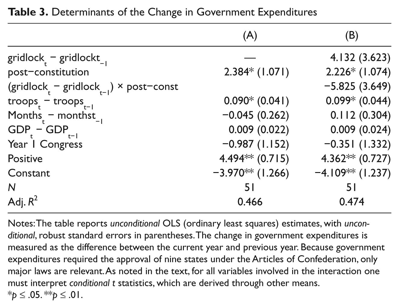
Notes: The table reports unconditional OLS (ordinary least squares) estimates, with unconditional, robust standard errors in parentheses. The change in government expenditures is measured as the difference between the current year and previous year. Because government expenditures required the approval of nine states under the Articles of Confederation, only major laws are relevant. As noted in the text, for all variables involved in the interaction one must interpret conditional t statistics, which are derived through other means.

p ≤ .05. **p ≤ .01.

The estimated coefficient for post-Constitution is positive and significant, indicating that the Constitution allowed for a significant increase in the change of government expenditures. In fact, with other variables held constant, the discrete change from the Articles of Confederation to the Constitution increased the ability to expand or contract government expenditures each year by US$2.4 million. This is a sizable amount considering that the average government expenditure was US$6.5 million under the Articles of Confederation and US$13.9 million under the Constitution.

The control variables appearing in the previous regression can be interpreted as stated previously. In addition, the dummy variable for a positive change in government expenditures is positive and significant, as expected. What is slightly more interesting is that, with the exception of troops, all the independent variables maintain the same sign and significance if this dummy is removed.¹⁸ This indicates broad support for claims that the Constitution enabled a more rapid expansion of government.

The Effect of the Gridlock Interval on the Volume of Statutes

The results of the previous sections suggest that the constitution facilitated more legislation and larger increases in government expenditures. If all we showed was evidence that the Constitution expanded government, then our findings would be limited. The more important insight is that the Constitution changed the government’s responsiveness to pivotal actors. This is shown in our next set of results.

Estimates for the complete version of specification (1) are presented in Table 2, Columns C and D. The sign and significance of the control variables are similar with similar interpretations. Hence, we focus on the interpretation of the gridlock interval and its interaction with the post-Constitution dummy.

Because the model is nonlinear and the gridlock interval is interacted with the post-Constitution dummy, the t statistics for grid interval, post-Constitution, and their interaction cannot be interpreted in the usual fashion (Brambor, Clark, & Golder, 2006). In other words, the stars (or lack of stars) on these variables can be misleading. Instead, we examine the effect of the gridlock interval on the predicted number of statutes using a graphical procedure outlined by Long and Freese (2006, pp. 436-437 & 440-441). For this analysis, we graph the predicted volume of statutes for various values of grid interval with year1 Congress held at its median and the other independent variables held at their means. For our pre-Constitution analysis, we set post-Constitution and the interaction term at zero. For our postconstitutional analysis, we set post-Constitution equal to 1 and the interaction term at the value of grid interval, which we allow to vary across its feasible range. This allows us to illustrate the predicted counts for all possible values of the gridlock interval.

Figure 3a displays the predicted number of statutes and 95% confidence intervals for minor issues. Post-Constitution conditions are depicted with thick lines, and pre-Constitution conditions are depicted with thin lines. The figure shows that the predicted number of minor statutes decreases slightly with larger gridlock intervals under the Articles of Confederation. This is significant for all possible values of the gridlock interval.¹⁹ Easier to see is a significant but fairly constant relationship between the number of statutes and the size of the gridlock interval under the Constitution. This relationship is significant only for values less than 1.1 (as shown by cases where the thick, dotted line exceeds 0). Comparing the two solid lines shows the Constitution is expected to produce more statutes than the Articles of Confederation for all gridlock intervals. However, the difference is significant only for gridlock intervals less than 1.0 (values on the x-axis where the 95% confidence intervals do not overlap). For gridlock intervals greater than 1.0 the two constitutions provide no statistically significant difference. The latter should not be a surprise because gridlock intervals greater than 1.0 are very constraining and neither constitution would be expected to produce much legislation with that level of gridlock. Because only two of the observed gridlock intervals exceed 1.0, the differences between the two documents are quite meaningful.

Figure 3.

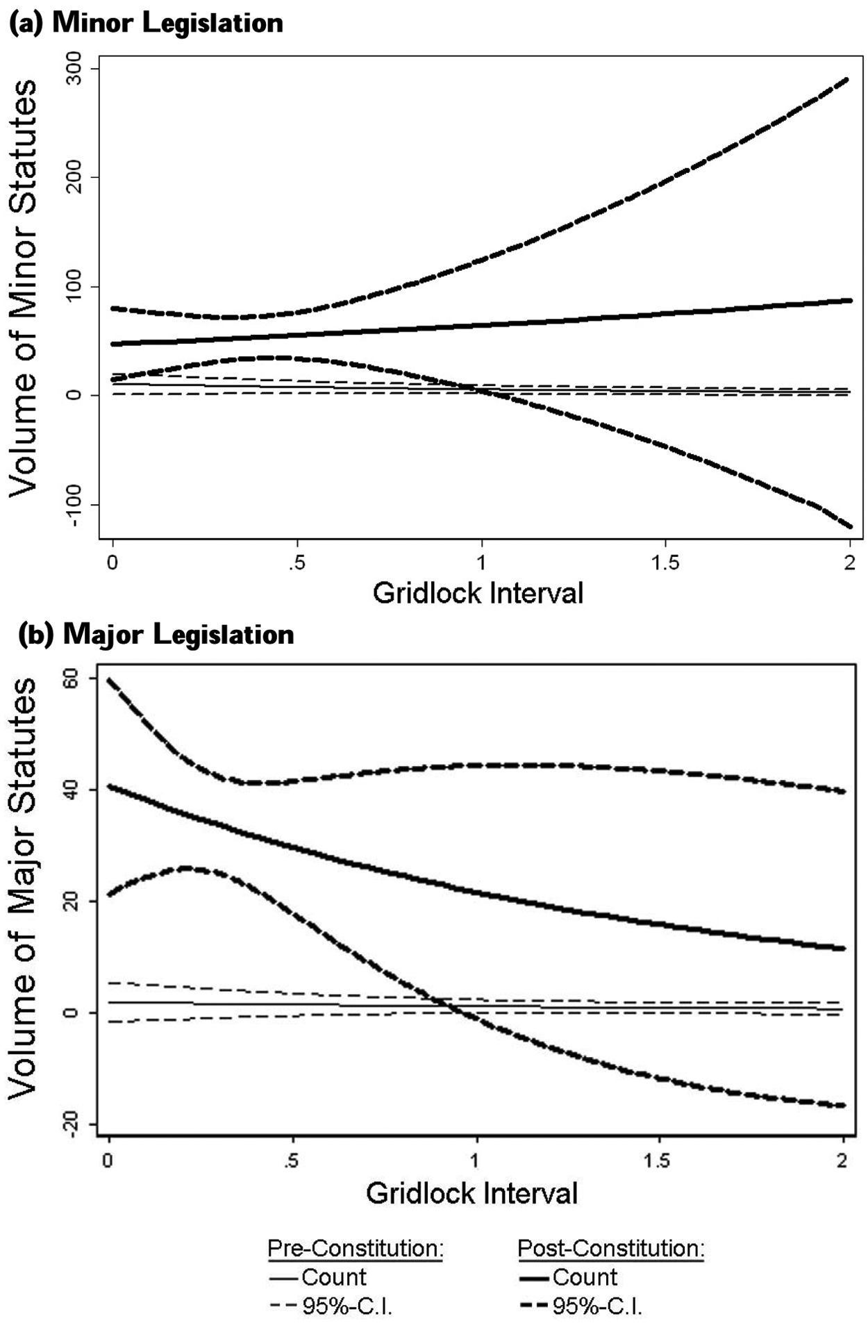
Predicted volume of legislation for various gridlock intervals

Figure 3b depicts similar results for major legislation. The thin solid line indicates that the predicted number of statutes decreases with greater gridlock intervals under the Articles of Confederation. However, the thin dashed line indicates that this relationship is never significant. In other words, the model predicts the Articles of Confederation would produce very few, if any, major statutes. Under the Constitution, the predicted number of statutes decreases as the size of the gridlock interval increases, and it is significantly greater than zero for gridlock intervals less than 1. Comparing the before and after cases shows a significant difference over the 0 to 1 range. Meaning, for most of the observed values of the gridlock interval, the Constitution produces many major statutes. The Articles of Confederation produces none. Furthermore, the slope of the relationship is considerably steeper under the Constitution than under the Articles of Confederation implying that the volume of legislation is more responsive to the length of the gridlock interval under the new document. The latter is what Madison, Hamilton, and other framers might have hoped.

A counterfactual history of the War of 1812 may help illustrate the magnitude of our finding. There should have been (and was) a large number of major statutes under the Constitution given the conditions of 1812. Our model predicts the nation should have produced 70 major statutes that year. However, with the exact same conditions but the earlier constitutional design (i.e., 1812 values of the independent variables with post-Constitution = 0) our model predicts the government would produce only three major statutes. This implies dramatically less legislation in a time of need. Without passage of the Constitution, the nation would have been considerably less capable of defending itself, vindicating the fears of Hamilton and other Federalists.¹

We also analyzed the conditional effect of post-Constitution (0 and 1) on the volume of legislation using a similar procedure (not shown). The results suggest the Constitution had a significant effect on the ability to enact legislation when the gridlock interval, and other factors, are controlled.

The Effect of the Gridlock Interval on Changes in Government Expenditures

Regression results for the complete version of specification (2) are presented in Table 3, Column B. We analyze gridlock intervals for major laws only, because nine states were required to pass government expenditures under the Articles of Confederation.

Because of the interaction term, the t values of the variables involved in the interaction are again misleading. We determined the conditional coefficients and conditional standard errors using techniques described by Friedrich (1982) and Brambor et al. (2006) but we do not report these conditional statistics in the table.²¹

Prior to the Constitution, changes in the gridlock interval have a positive but insignificant effect on changes in government expenditures. After enactment of the Constitution, changes in the gridlock interval have a negative and significant effect on changes in government expenditures at the .10 level. This demonstrates that changing the size of the gridlock interval has a marked effect on changing government expenditures under the Constitution, but no effect under the Articles of Confederation. In fact, with all other variables held constant, a 0.10 increase in the gridlock interval corresponds to a US$92,631 decrease in government expenditures under the Constitution. Given the relatively low levels of government spending, this represents a tremendous improvement in the ability of the government to change expenditures in response to legislative preferences.

Again, our War of 1812 example may help illustrate the effect. In 1812 the U.S. government recorded expenditures of US$19.1 million, an increase of US$11.4 million from the previous year. Our model predicts that with all variables held at their 1812 values, the government should have increased expenditures by US$3.1 million. However, if post-Constitution was set at its pre-Constitution value, then the government should expect no increase in expenditures as a result of changing the gridlock interval. As a result, the nation would have been much less effective at raising expenditures and less effective at responding to the British under the old constitutional design.

Furthermore, we find that post-Constitution is positive and significant for most changes in the gridlock interval. Using .10 as the significance level, post-Constitution is significant for all (gridlock_t − gridlock_t−1) < 0.078. This is 86% of the observed data. Hence, changing constitutions had an important effect on the nation’s ability to change government expenditures, consistent with our previous finding.

Other Constructions of the Gridlock Interval

To check the robustness of our results, we considered two other constructions of our gridlock intervals. First, some authors suggest that early American presidents would exercise the veto only if a bill was unconstitutional (McGowan, 1986; Spitzer, 1988). Put differently, they claim such presidents would rarely veto. Although there is reason to question this claim (McCarty, 2009), we can model the practice of rarely if ever exercising the veto by removing the Presidents (and subsequently the two-thirds overrides) from the gridlock interval. The gridlock interval is then constructed as the distance between the median member of the House and the median member of the Senate post-Constitution. Gridlock intervals from the Articles of Confederation remain the same. Conducting the analysis under these assumptions produces similar results for both statutes and government expenditures.²² Furthermore, the conditional analysis depicted in Figures 3 and 4 suggests that enactment of the Constitution increases the effect of the volume of legislation for some values of the gridlock interval, albeit over a smaller range.

Second, since much of the gridlock literature stresses the importance of political parties, some scholars might object to the omission of parties. As a result, we also considered a model that assumes that the median member of the majority party was the pivotal member of each chamber for the fourth through the seventeenth Congresses.²³ We also assume that all legislators can propose as before, implying that no point is in equilibrium solely because the proposer is dilatory. The algorithm for creating such a gridlock interval is identical to the one in the Appendix, except chamber medians are replaced by medians of the majority party. Gridlock intervals for other years remain the same. Conducting an analysis similar to the analyses presented in Figures 3a and 3b suggests that the Constitution has a significant effect on the volume of legislation for greater ranges of the gridlock interval with parties included. With one exception, the sign and significance of all other conditional variables remain the same.²⁴

Conclusion

Our results show that the Constitution produced a more expansive national government during a period when many believed the government needed to expand. The positive and significant relationship of the post-Constitution dummy indicates that with other variables held at their means, the enactment of the Constitution should create 58 more minor statutes per year, 32 more major statutes per year, and an additional US$2.4 million change in government expenditures.

If this article showed no more, then scholars who favor smaller and less active government might find reason to favor the Articles of Confederation. It was difficult to change policy under the Articles of Confederation, which some scholars find desirable (Holcombe, 1991; Sobel, 1999). However, without knowing the circumstances, there is no reason to want a government that is particularly adept at passing proposals or particularly adept at rejecting them. What an institutional designer should prefer is a government that allows for policy change when elected officials largely agree change is needed and maintains the status quo when elected officials largely agree they should stay the course. In other words, they should want government to be more responsive to changes in the gridlock interval.

Our second result on the marginal effect of the gridlock interval pre- and post-Constitution shows that the Constitution made this type of improvement for major statutes—both in terms of the value of legislation and the change in government expenditures. Under the Constitution, the volume of major statues largely decreased with increasing sizes of the gridlock interval and increased with decreasing sizes of the gridlock interval (Figure 3b). The gridlock interval had no effect on major statutes under the Articles of Confederation. This suggests that the Constitution not only increased the outputs of government but also made government more responsive to the preferences of pivotal actors. Furthermore, under the Constitution a 0.1 increase (decrease) in the gridlock interval corresponded to a US$92,631 decrease (increase) in government expenditures—roughly 12% of the average post-Constitution expenditures. Under the Articles of Confederation, the gridlock interval had no effect on government expenditures. In the latter case, government was small regardless of legislative, and presumably constituent, preferences. Again, this indicates that the Constitution made government policy more responsive to the gridlock interval itself and more responsive to the key legislative preferences that are implied by the constitutional design. It is for this reason that one might consider government under the Constitution more effective.

Although we do not want to generalize too hastily, these results provide some initial evidence that presidential systems may be more reflective of demand for political initiatives than confederal systems. In which case, we do not need to choose between a system that typically prevents action or one that typically enables action. We can have our cake and eat it too. We can choose systems that are effective when all the pivotal actors demand effectiveness and stable when pivotal actors demand stability. Such distinctions are important for framers of modern confederative designs, such as the United Nations and the African Union. Framers of those systems may want to protect state sovereignty and maintain the status quo, but perhaps they can achieve their goals without creating a completely ineffective government.

Footnotes

Appendix: Data Construction and Sources

To calculate gridlock intervals, we first estimate the spatial location of each delegate in a single dimension using a pooled roll call matrix which includes all actors and all roll calls from August 1, 1777 to March 3, 1829. This matrix contains 1,772 legislators (including presidents) and 7,609 roll calls; 1,593 of the roll calls were prior to the Constitution. Data for 1777-1788 came from Lord (1984), while roll call data for 1789-1829 came from the Poole and Rosenthal website.²⁵ Because DW-NOMINATE is inappropriate for this study,²⁶ spatial locations were estimated using W-NOMINATE with Rufus King as the left restriction. By estimating the location of legislators using a single matrix, we implicitly create a common space for all the legislators and assume each delegate is in a fixed location throughout his/her career.

To test whether this provides a common space, we use a procedure developed by Poole (2005). The results indicate that the pre and post-Constitution periods share enough in common to be used as a comparable, single dimension.²⁷ Such findings are consistent with the historical arguments made by Aldrich and Grant (1993) and Aldrich et al. (2002) who claim that the periods have a “clear commonality in people, preferences, and policy choices” but “stark differences in institutions and outcomes” (Aldrich et al., 2002, 317). We conjecture that our single dimension reflects views about the relative strength and authority of the national government, with greater pro-nationalism on the left side.²⁸ A skree plot of the eigenvalues of the double-centered agreement score matrix suggests that a single dimension accounts for much of the variance in legislative votes from 1777 to 1829.²⁹

For legislation under the Articles of Confederation, we first calculate the gridlock interval monthly to address attendance issues (using attendance data gathered from Smith and Gephart 2000). We treat a delegate as attending a particular month if he attended at least five days. We then determine the left and right pivots for each delegation each month. For an odd sized delegation, these pivots are the same median voter. Next, we determine the left and right pivots of the chamber using the median delegates from each of the states. Gridlock intervals are then calculated as the difference between the right and the left floor pivot each month. For each year, we report the monthly average of the gridlock interval.

Although one might think that if seven or more states attended, the gridlock interval for minor legislation would reduce to a single median point, this never occurred in our data, partly because all thirteen states never attended at the same time. Since motions required the approval of a majority of the states in the confederation, not a majority of the states present, seven states often became a supermajority of the states attending which caused the equilibrium to be a range.³⁰ Poor attendance partly explains why gridlock intervals under the Articles of Confederation were large. However, a comparison of state attendance and the gridlock intervals suggests that state attendance was not fully responsible for variation in the gridlock interval.

Calculating gridlock intervals under the Constitution was considerably easier. For each year we first determined the median voter of each chamber (paying particular attention to even sized chambers where the median is likely to be a range) as well as the left 2/3rds and right 2/3rds pivots. We then recorded the president’s ideal point and calculated gridlock intervals using the following algorithm.

if (H ≤ P ≤ S) or (S ≤ P ≤ H), then grid = | H−S |

else {if (H < P & S < P), { then

if (Hr ≤ P & Sr ≤ P), then grid = | min(H, S) − max(Hr, Sr) |.

else grid = | min(H, S) − P |.}

if (P < H & P < S), { then

if (P ≤ Hl & P ≤ Sl), then grid = | max(H, S) − min(Hl, Sl) |.

else grid = | max(H, S) − P | }}

where H is the median of the House; S is the median of the Senate; P is the location of the President, Hl and Sl are the left two-third pivots of the House and Senate, respectively; Hr and Sr are the right two-third pivots of the House and Senate, respectively; and grid is the length of the gridlock interval. In cases where the number of members of a chamber were even, the majority pivot farthest from the President was used.

In each case, we assume that all players can propose. This makes the gridlock interval typically smaller than the gridlock intervals used by Krehbiel (1998) because it removes cases where a status quo is in equilibrium solely because the designated proposer objects.

The sources of the remaining variables are described in Table 4.

Acknowledgements

The authors would like to acknowledge Ryan Bakker, Tony Bertelli, and Damon Cann for useful discussions regarding our empirical specifications, Michael Malbin for explaining his presidential request data, and Keith Poole for providing an upgraded version of W-NOMINATE for large matrices.

Declaration of Conflicting Interests

The author(s) declared no potential conflicts of interest with respect to the research, authorship, and/or publication of this article.

Funding

The author(s) received no financial support for the research, authorship, and/or publication of this article.

Notes

Bios

Keith Dougherty is an associate professor of political science at the University of Georgia. His research interests focus on the design of American political institutions.

Justin Moeller is an assistant professor of political science at Eastern University. His research interests include American political development, political parties, and campaigns and elections.

References

Aldrich

J. H.

(1995). Why parties?: The origin and transformation of political parties in America. Chicago, IL: The University of Chicago Press.

Aldrich

J. H.

Grant

R. W.

(1993). The Antifederalists, the first Congress, and the first parties. The Journal of Politics, 55, 295-326.

Aldrich

J. H.

Jilson

C. C.

Wilson

R. K.

(2002). Why Congress? What the failure of the Confederation Congress and the survival of the Federal Congress tell us about the new institutionalism. In Brady

McCubbins

(Eds.), Party, process, and political change in Congress (pp. 315-342). Stanford, CA: Stanford University Press.

Baker

(2009, September 17). Expand the House? New York Times.

Beth

R. S.

(2005). Entrenchment of Senate procedure and the “Nuclear Option” for change: Possible proceedings and their implications. Congressional Research Service, RL32843.

Brady

D. W.

Volden

(2006). Revolving gridlock: Politics and policy from Jimmy Carter to George W. Bush. Boulder, CO: Westview.

Brambor

Clark

W. R.

Golder

(2006). Understanding interaction models: Improving empirical analyses. Political Analysis, 14, 63-82.

Brown

R. H.

(1993). Redeeming the republic: Federalists, taxation, and the origins of the Constitution. Baltimore, MD: Johns Hopkins Press.

Chiou

Rothenberg

L. S.

(2003). When pivotal politics meets partisan politics. American Journal of Political Science, 47, 503-522.

10.

Chiou

Rothenberg

L. S.

(2008). Comparing legislators and legislatures: The dynamics of legislative gridlock reconsidered. Political Analysis, 16, 197-212.

11.

Coulson

D. P.

Joyce

(2003). United States state-level population estimates: Colonization to 1999. Washington, DC: United States Department of Agriculture.

12.

Ferguson

J. E.

(1961). The power of the purse: A history of American public finance, 1776-1790. Chapel Hill: University of North Carolina Press.

13.

Fisk

Chemerinsky

(1997). The filibuster. Stanford Law Review, 49, 184-254.

14.

Friedrich

R. J.

(1982). In defense of multiplicative terms in multiple regression equations. American Journal of Political Science, 26, 797-833.

15.

Garfinkel

M. R.

Skaperdas

(2007). Economics of conflict: An overview. In Hartley

Sandler

(Eds.), Handbook of defense economics (Vol. 2, pp. 649-709). New York, NY: Elsevier.

16.

Gartner

S. S.

(2006). Military personnel on active duty, by branch of service and sex: 1789-1995. In Carter

S. B.

Gartner

S. S.

Haines

M. R.

Olmstead

A. L.

Sutch

Wright

(Eds.), Historical statistics of the United States: Millennial edition (Table Ed 26-47). New York, NY: Cambridge University Press.

17.

Holcombe

R. G.

(1991). Constitutions as constraints: A case study of three American constitutions. Constitutional Political Economy, 2, 303-328.

18.

Jacobs

J. R.

(1947). The beginning of the U.S. Army, 1783-1812. Princeton, NJ: Princeton University Press.

19.

Jillson

C. C.

Wilson

R. K.

(1994). Congressional dynamics: Structure, coordination, and choice in the first American Congress, 1774-1789. Stanford, CA: Stanford University Press.

20.

Jensen

(1965). The new nation: A history of the United States during the confederation 1781-1789. New York, NY: Alfred A. Knopf.

21.

Krehbiel

(1998). Pivotal politics: A theory of U.S. lawmaking. Chicago: University of Chicago Press.

22.

Long

J. S.

(1997). Regression models for categorical and limited dependent variables. Thousand Oaks, CA: SAGE.

23.

Long

J. S.

Freese

(2006). Regression models for categorical dependent variables using Stata. College Station, TX: Stata Press.

24.

Lord

(1984). Roll calls of the Continental Congresses and the Congresses of the Confederation, 1777-1789 [Data file]. ICPSR # 7537.

25.

McCarty

(2009). Presidential vetoes in the early republic: Changing constitutional norms or electoral reform? Journal of Politics, 71, 369-384.

26.

McCormick

R. P.

(1966). The second American party system: Party formation in the Jacksonian Era. Chapel Hill: The University of North Carolina Press.

27.

McCusker

J. J.

(2006). Gross domestic product: 1650-1800. In Carter

S. B.

Gartner

S. S.

Haines

M. R.

Olmstead

A. L.

Sutch

Wright

(Eds.), Historical statistics of the United States: Millennial edition (Table Eg. 217-222). New York, NY: Cambridge University Press.

28.

McGowan

(1986). The president’s veto power: An important instrument of conflict in our constitutional system. San Diego Law Review, 23, 791-822.

29.

Mondale

W. F.

(2011, January 1). Resolved: Fix the filibuster. New York Times.

30.

Pitkin

(1980). A statistical view of the commerce of the United States of America. New York, NY: Goldsmiths Kress Library of Economic Literature No. 21731. (Original work published 1817)

31.

Poole

K. T.

(2005). Spatial models of parliamentary voting. New York, NY: Cambridge University Press.

32.

Smith

P. H.

Gephart

R. M.

(Eds.). (2000). Letters of delegates to Congress, 1774-1789 (Vol. 26). Washington, DC: US Government Printing Office.

33.

Sobel

R. S.

(1999). In defense of the Articles of Confederation and the contribution mechanism as a means of government finance: A general comment on the literature. Public Choice, 99, 347-356.

34.

Spitzer

R. J.

(1988). The presidential veto: Touchstone of the American presidency. Albany, NY: SUNY Press.

35.

Stewart

R. W.

(2005). American military history. Washington, DC: Center of Military History, U.S. Army.

36.

Sutch

(2006). Gross domestic product: 1790-2002. In Carter

S. B.

Gartner

S. S.

Haines

M. R.

Olmstead

A. L.

Sutch

Wright

(Eds.), Historical statistics of the United States: Millennial edition (Table Ca 9-19). New York, NY: Cambridge University Press.

37.

Swift

E. K.

Brookshire

R. G.

Canon

D. T.

Fink

E. C.

Hibbing

J. R.

Humes

B. D.

. . . Martis

K. C.

(2000). Database of Congressional historical statistics, 1789-1988 [Data File]. Ann Arbor, MI: ICPSR.

38.

U.S. Printing Office. (1845). The public statutes at large of the United States of America (Vols. 1-4). Boston, MA: Little, Brown.

39.

U. S. Printing Office. (1937). Journals of the Continental Congress, 1774-1789 (ed. Ford

W. C.

, 34 Vols.). Washington, DC: Author.

40.

U.S. Treasury Department. (1832). American state papers, Military affairs. Washington, DC: Gales and Seaton.

41.

Wallis

(2006). Federal government finances—revenue, expenditure, and debt: 1789-1939. In Carter

S. B.

Gartner

S. S.

Haines

M. R.

Olmstead

A. L.

Sutch

Wright

(Eds.) Historical statistics of the United States: Millennial edition (Table Ea 584-587). New York, NY: Cambridge University Press.

42.

Zernike

(2010, December 19). Proposed amendment would enable states to repeal federal law. New York Times.