Time Regulations as Electoral Policy

Abstract

Having had more or less sleep changes mood and behavior; for example, more sleep associates with greater productivity and a perception that more time is available. This changes the time cost of voting in ways particularly important for the United States, where the general elections are sometimes but not always held 2 days after a 25-hr day, when people typically have had more time to catch up on sleep. Election returns and surveys confirm that circumstances where the election occurs 2 days after a long day produce higher turnout, suggesting a role for factors that affect sleep in political behavior.

Keywords

turnout voting sleep daylight saving time circadian rhythm

In non-tropical parts of the world, daylight hours shift over the course of the year. To align hours of natural light with hours of human activity, many governments mandate “daylight saving time” (or “summer time”): a seasonal misalignment of the clock, shortening one spring day and lengthening one autumn day by an hour. These changes in day length affect sleep patterns for several subsequent days (Lahti, Leppämäki, Lönnqvist, & Partonen, 2006), perturbing circadian rhythms (Kantermann, Juda, Merrow, & Roenneberg, 2007) and altering mood, alertness, and time available. The consequences are often innocuous, but major events can arise in these atypical periods. In particular, many years’ autumnal clock shift occurs just 2 days before the United States’ general election, so the electorate has more time to be caught up on sleep and so has more time to vote. Turnout might then be higher than in otherwise similar places lacking seasonal clock changes, or than in years where the clock shifts after or well before the election.

This article assesses clock-shift effects in several ways. One test looks at counties within the state of Indiana, which was long split between areas that did and did not shift their clocks. Another test uses state-level data to look for macro-level impacts that pre-election clock shifts might have. Finally, a third approach considers survey responses: Do more people report voting when their election occurred the same week as a 25-hr day? All three analyses find higher turnout when the weekend preceding the election contained an extra hour. The survey results additionally suggest that the effects are strongest, as would be expected, among those whose propensity to vote is uncertain—that is, among those who are not habitual voters. While the estimated effects of recent clock shifts involve only a couple of percentage points of the population, this nevertheless, because of its wide impact, implies a large number of citizens for whom the presence of more hours in a recent day was pivotal for voting.

Shifting Clocks and Behavior

Changing the length of a day alters physiological circadian rhythm in several dimensions (Lavie, 2001; Mills, 1966), notably by interrupting sleep (Ohayon, Smolensky, & Roth, 2010). Changed sleep, in turn, disturbs biological processes and modifies human behavior. Sleep deprivation affects everything from cognition to motor skills, producing worse moods and lower performance (Pilcher & Huffcutt, 1996). This changes decision-making (for example, by affecting moral reasoning; Olsen, Pallesen, & Eid, 2010). Conversely, a bonus hour of sleep, even from a normal, not sleep-deprived baseline, measurably enhances mood and productivity—as well as other mental and physical functioning—for several days (Monk & Aplin, 1980). Most individuals adjust to such sleep variations within a week, although a few show effects of the disruption for more than a fortnight (Valdez, Ramírez, & García, 2003).

A widespread source of this sort of 1-hr shift in sleep schedules is daylight saving time. This process of shifting clocks occurs in much of North America, Europe, and the Middle East, as well as some parts of South America and Oceania. In places with daylight saving time, clocks are, in the spring, shifted forward by an hour relative to the local standard time, only reverting to the local standard time in the autumn. Most people react to such clock changes by abruptly cutting sleep by an hour in the spring or taking an extra hour of sleep in the autumn, so that the changeovers lead much of the population to be more or less sleep deprived than usual. Although some are skeptical of how much these shifts matter (Michelson, 2011), scholars have linked them to many measurable social effects. The largest literature concerns upticks in traffic and workplace accidents in the aftermath (e.g., Barnes & Wagner, 2009), but effects crop up across a range of outcomes, including stock market volatility (Kamstra, Kramer, & Levi, 2010), energy use (Kotchen & Grant, 2011), and online malingering at work (Wagner, Barnes, Lim, & Ferris, 2012). Transitions surrounding daylight saving time may also associate with heart attacks (Janszky & Ljung, 2008) and episodes of mental illness (Lahti, Haukka, Lönnqvist, & Partonen, 2008), though empirical evidence on these health-related conjectures is mixed.

Despite the pervasive influence of these policies, their political implications have gone essentially unremarked. The most prominent study of daylight saving time in political science (Shipan, 1996) used it only as a case of competition between legislative committees, and studies at the intersection of politics and sleep disruption have generally considered the former as a cause of the latter, not the other way around (e.g., Sadavoy, 1997; Schredl & Piel, 2006). Yet clock shifting might be of great interest to political analysts, particularly in the United States, where it occurs at a key point in the electoral calendar. The Uniform Time Act of 1966 mandated that daylight saving time would be in place until the last Sunday in October. As of 2007, the Energy Policy Act of 2005 moved this ending point to the first Sunday of November. These dates happen to verge on the date of American federal elections: Since 2007, the election occurs 2 days after the autumn clock shift in any year that November does not start on a Monday (as it did in 2010, and will again in 2021). Prior to 2007, the election happened 2 days after the clock change only in years when November started on a Monday (as it did in 2004 and, before that, in 1999).

In some years, then, the end of daylight saving time hits potential voters very shortly before the election. As the extra hour is consumed over subsequent days, the time costs of voting decline, so that turnout should increase (Gibson, Kim, Stillman, & Boe-Gibson, 2013). That is, close proximity between elections and the end of daylight saving time may bring to the polls people who would otherwise not have voted, and locations that shift their clocks would be predicted to have higher turnout rates in affected years. Because, as noted above, the effect of a change in sleep tends to dissipate over approximately a week, the clock shift is likely to have a far smaller impact when it occurs 9 days before the election (as was the case in most pre-2007 years) or 5 days afterward (as periodically happens with the post-2007 calendar). These differences in calendar across years are plausibly exogenous to most social factors, making for relatively clean empirical tests. However, years when November starts on Monday are also those when elections occur on November 2, the earliest possible date, when, for example, average weather is slightly warmer than for later election dates. Such differences between dates in early November are likely to be trivial, but nonetheless slightly contaminate cross-year comparisons on the effect of clock shifts.

Besides differences across years, places also differ in their observance of daylight saving time: Even within particular years, daylight saving time affects people in divergent ways. Arizona has mostly opted out of daylight saving time, citing increased air-conditioning cost when people’s active hours are in the height of the day. Hawaii’s low latitude makes seasonal variation in daylight too small to make clock shifts worthwhile. Michigan and Indiana have not always observed daylight saving time, because being on the edge of their time zones means that daylight saving time seriously misaligns clock and solar time. Michigan abstained from 1969 through 1972 before re-joining the daylight-saving-time system, while Indiana’s varied choices are further presented below.

This suggests multiple potential avenues for studying how daylight saving time affects turnout. One considers how electoral participation differs in years when the election falls just 2 days after the time shift instead of occurring 9 days after or 5 days before. Another looks at how election results within a year differ between places that follow daylight saving time and those that do not. The analyses below look at both of these dimensions of variation. Moreover, the analyses use both individual survey responses, which allow controls for personal-level characteristics, and geographically aggregated turnout statistics, which avoid validity concerns surrounding survey respondents’ tendency to over-report turnout (Karp & Brockington, 2005).

Indiana

Indiana exemplifies both dimensions of variation and so is an obvious place to start the analysis. With its location on the border between Eastern and Central time zones, the state split according to whether the local population had closer economic ties to points east or points west. Counties that chose Eastern time were, in effect, on daylight saving time year-round, and most (but not all) of them rejected the further misalignment of clocks that shifting clocks forward an additional hour would require. Moreover, counties changed their regulations over time. In elections from 1968 to 1972, 17 Indiana counties had daylight saving time; the tally fell to 16 from 1974, 15 from 1978, and 14 from 1990. Finally, in 2006, to allay confusion, the state adopted daylight saving time statewide.¹ This unusual history allows for variation with respect to exposure to shifts in the clock just before the election while holding constant factors specific to a particular (statewide) campaign, such as competitiveness or intensity of campaign advertising. In years having a clock shift just before the election (1976, 1982, 2004, and 2008), only those parts of Indiana observing daylight saving time would be expected to have altered turnout rates. Years when daylight saving time ends more than a week before the election (or when daylight saving time was universal throughout the state) cross-check whether a county simply has a higher turnout rate regardless of clock-based effects.

To operationalize this, the primary dependent variable is the proportion of those registered in each of Indiana’s 92 counties² who cast a ballot in a given year’s general election. Registered voters are a reasonable basis for calculating turnout for this case: Registration procedures are relatively consistent within the state of Indiana in ways they are not in multi-state comparisons, and the unavailability of same-day registration means that only the registered can make last-minute decisions to vote and so be affected by changes in the clock just before the election. This information is available for every biennial election from 1990 to 2010.

This basic turnout measure includes some individuals who voted absentee. Because absentee ballot requests were due before the clock shift had a chance to influence behavior, such voters may not be relevant to the hypothesis considered here. Accordingly, another measure might calculate turnout only among those who did not vote absentee:

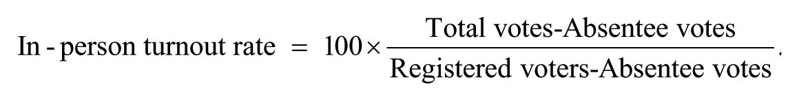
In - person turnout rate = 100 \times \frac{Total votes - Absentee votes}{Registered voters - Absentee votes} .

Absentee ballot information is not available for the 1998 election or for Newton County in 1994, so the in-person rate is also missing for these observations.

Because Indiana’s daylight-saving-time counties were mostly those in multi-state metropolitan areas, various demographic factors likely affect counties’ likelihood of experiencing a clock shift before the election as well as turnout rates. These include the electorate’s racial composition, measured by Census estimates of the White and Black shares of the local population as of July of the given election year, and the local age distribution, measured with the year’s Census estimate of the proportion of the population over 65. To account for economic factors, the models include both the county’s unemployment rate (as reported by the Bureau of Labor Statistics for the month of the election) and the change in that unemployment rate over the previous 3 months. The models also, to measure urbanness directly, control for the (natural logarithm of) population per square mile of county land area. Finally, Indiana allows for fixed effects for (i.e., indicator variables for each level of) year and county. These subsume secular trends or influences wrought by the Energy Policy Act or by 2010’s anomalous post-election clock shift and allow for difference-in-difference estimation of the clock-shift effects.

Table 1 displays the ordinary least-squares regression results. Whether using overall or in-person turnout rates, recent clock shifts associate with an approximately 2.5-percentage-point increase in predicted turnout. While this effect attains only marginal levels of statistical significance, the point estimate is credible in comparison with the effects of the control variables: It has roughly the same effect as increasing a jurisdiction’s over-65 population by 5 percentage points, for example. Few of the substantive control variables see statistically significant effects, perhaps because the county fixed effects capture much of the relevant variation. However, more densely populated counties do appear to have a higher turnout, all else equal, perhaps because people tend to live nearest to their voting place in urban areas (Gimpel & Schuknecht, 2003).

Table 1.

OLS Models of Percent Registered Voters Who Cast Ballots in Indiana Counties (1990-2010).

	All turnout	In-person turnout
Clocks change 2 days before election	2.57 (1.536)	2.56 (1.521)
Percent population White	−0.89 (0.479)	−0.23 (0.527)
Percent population Black	−0.76 (0.762)	−0.07 (0.841)
Percent population at least 65 years old	0.40 (0.286)	0.65 (0.301)
Unemployment rate, month of election	0.04 (0.151)	0.07 (0.155)
3-month unemployment rate change	−0.08 (0.213)	−0.08 (0.218)
Natural log, people per square mile	7.60 (3.620)	8.86 (3.719)
n	1,012	919

Note. Year fixed effects are included but are suppressed; robust standard errors are given in parentheses. OLS = ordinary least squares.

States

Indiana’s idiosyncratic patchwork of standards may sensitize its residents to time-related factors. When considering electoral effects, its polls’ early closing time might do so as well: Evening daylight³ normally correlates with more turnout (Rallings, Thrasher, & Borisyuk, 2003), but Indiana’s unusual 6:00 a.m. to 6:00 p.m. poll hours may make sunrise as relevant. To see whether clock shifts matter more broadly, this section looks for similar effects across state-years. (“State” here generically includes the District of Columbia, though its exclusion does not appreciably change reported results.) State-level data have the additional advantage of including some states (Kentucky, Mississippi, New Jersey, and Virginia; Louisiana state elections, falling on Sunday, have a different temporal relationship to clock shifts and so are excluded) with state-level elections in odd-numbered years, allowing for more years (1971, 1993, 1999, 2007, 2009, and 2011) with clock shifts 2 days before the election.

Using an indicator of whether state-years saw clock shifts just before elections is mostly unproblematic, with two exceptions. One is Indiana with its hopelessly mixed policy; reported models in this section exclude the state, although including it for years when it adopted statewide daylight saving time produces very similar results. The other is Arizona: the Navajo Nation observes daylight saving time, whereas the rest of Arizona does not. This taints Arizona data with some population that may have experienced a clock shift just before the election. However, the Navajo Nation population is a relatively small fraction of Arizona’s (falling over the period here from around 7% of the state to around 2.5%), and any bias from misidentification should conservatively reduce effect sizes by reducing the difference between levels of the independent variable.

For the dependent variable, the basic measure here is Michael P. McDonald’s measure of voter turnout as a share of the voting-eligible population (McDonald, 2002). This measure, which improves comparison across states by accounting for differences in non-citizen or disenfranchised populations, is available (for even-numbered, federal-election years only) from 1980 through 2010, although McDonald’s data anomalously lack information for Louisiana in 1982. To ensure that uncertainty in the corrections for voting eligibility does not drive results, an alternative measures the number of votes cast as a fraction of the Census’s estimated voting-age population; this measure is available for most state-years from 1971 through 2011.

For control variables, state fixed effects account for differences in state culture that influence voting as well as likelihood of adopting policies such as daylight saving time. To capture the effect of different elections in a state, the models include indicators of whether the state-year features a presidential or gubernatorial election and a count of the number of local Senate races. A linear time trend, and an indicator for whether the state-year postdates the Energy Policy Act’s shift in daylight saving time policy, accounts for variation in voting behavior over time. Finally, as a particularly influential electoral policy that has, like pre-election clock shifts, recently become more common, the models indicate whether the state-year allowed for election-day registration.

Table 2 presents the results; having an extra hour in the day just before the election again associates with more voting. Here, the estimated turnout increase is 4.5 percentage points using the voting-eligible population measure. This is atypically large compared with the estimates from Indiana, though the estimate returns to being somewhat less than 3 percentage points using the voting-age population measure. These estimates easily attain standard benchmarks of statistical significance, and are somewhat larger than the predicted effects of having a gubernatorial or senatorial race in the state. Other control variables also have plausible coefficient estimates: Presidential races stimulate predictably massive increases in turnout, while recent elections have seen rates of participation above the historical trend. Election-day registration sees little effect in these models, likely because of its correlation with underlying state-level effects.

Table 2.

OLS Models of Voter Turnout, by U.S. State (Excluding Indiana).

	% Eligible voters	% Voting-age population
Clocks change 2 days before election	4.51 (0.416)	2.63 (0.408)
Presidential election	15.78 (0.425)	15.85 (0.398)
Gubernatorial election	1.66 (0.432)	2.77 (0.406)
Senatorial election(s)	1.32 (0.316)	1.04 (0.302)
Year	0.07 (0.019)	−0.02 (0.016)
Post-Energy Policy Act year	1.00 (0.534)	1.07 (0.589)
Election-day registration	−0.57 (1.247)	0.54 (1.015)
Odd-numbered year		−1.32 (1.082)
n	799	1,068

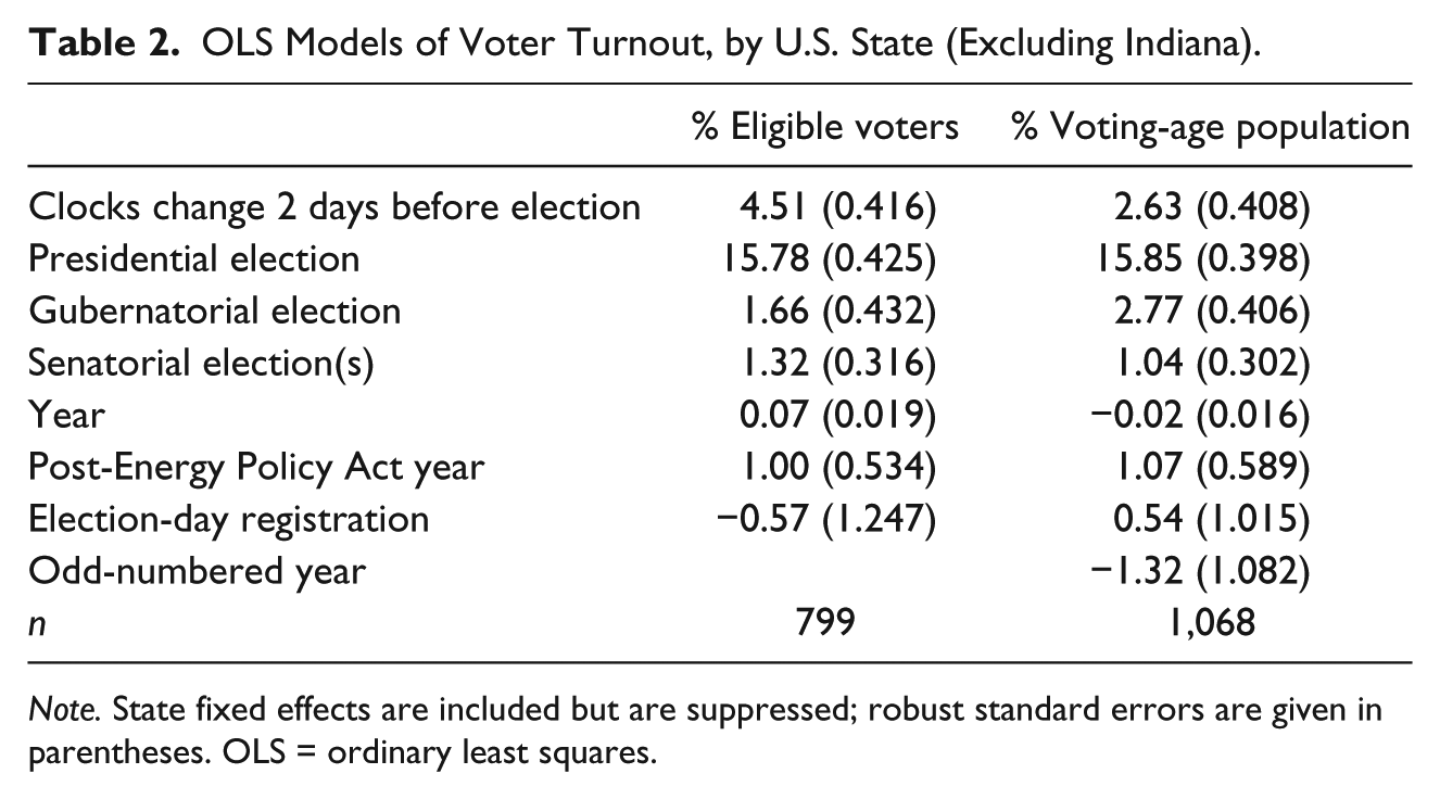
Note. State fixed effects are included but are suppressed; robust standard errors are given in parentheses. OLS = ordinary least squares.

Survey Responses

To explore the effect of daylight saving time’s end on turnout in a survey, the ideal data source would have information across years and places. One such data source is the American National Election Study (ANES), which has asked respondents nationwide about their voting behavior since before the Uniform Time Act standardized the United States’ observance of daylight saving time. The primary independent variable of interest is whether the respondent resides in a place where local time shifted by an hour exactly 2 days before the election.

In this survey, the dependent variable, electoral participation, is a simple indicator equal to 1 when the respondent reports having cast a ballot in the election and 0 otherwise. As with the Indiana models, an alternative measure excludes those who voted absentee and thereby did not make an Election-Day decision about voting. The ANES only systematically collected information on early and absentee voting from 1994, so focusing only on Election-Day voters excludes the earlier years’ data (as well as respondents from later years who did vote early). Despite its necessarily smaller sample, looking only at this narrower measure of turnout offers a check that the causal mechanism in question is actually animating any observed results.

For control variables, state of residence is an obvious issue, so the models include a full battery of indicator variables for states. To account for changes in policy over time, with more widespread adoption of daylight saving time and the alteration in daylight saving time’s schedule from 2007 on, the models below, like in Table 2, include controls for year of survey, an indicator of whether the year involved was after the implementation of the Energy Policy Act, and an indicator of whether the state-year allowed voters to register on Election Day. Year-level effects also associate with cross-year differences in which offices are up for election, which can exert strong influences on turnout. To account for this, three variables code if the respondent was in a state-year having presidential, gubernatorial, and (federal) senatorial elections. The first two of these variables are indicator variables, while the third counts how many U.S. Senate seats were on the ballot for the given state-year. Individual-level factors are perhaps less likely to condition one’s willingness to live in a jurisdiction with shifting clocks. Nevertheless, they merit inclusion in the model because their absence from the model may produce such large prediction errors as to render all estimates unreliable. These include controls for such demographic factors as age (in years), age squared, femaleness (measured with an indicator variable), and belonging to a racial or ethnic minority (also coded with an indicator). The models also include measures of education (on a 4-point scale), income (on a 5-point scale), and intensity of partisanship (on a 4-point scale), as generally important predictors of electoral participation.

The first two columns of Table 3 report the model results, using logistic regression (because the dependent variable of having reported voting is a binary variable). In both models, a clock change just before the election associates with higher probability of voting. The magnitude of that effect is somewhat smaller than the predicted effect of having a gubernatorial election in a state; for someone at median levels of the control variables, the estimated probability of voting increases by around 2 percentage points after a clock shift. The effect has only modest statistical significance when using the all-voter turnout measure (two-tailed p = .072), though the effect for in-person day-of-poll voting is more confidently estimated.

Table 3.

Logistic Model of Individual Turnout (1972-2008), From ANES Data.

	Baseline model	No early voters	Interaction
Clocks change 2 days before election	0.10 (0.058)	0.50 (0.163)	0.14 (0.062)
Predicted habitual voter			0.03 (0.052)
Clock change × Habitual voter			−0.13 (0.072)
Presidential election	1.09 (0.062)	1.37 (0.188)	1.09 (0.065)
Gubernatorial election	0.15 (0.073)	0.57 (0.228)	0.15 (0.073)
Senatorial election(s)	0.03 (0.041)	0.10 (0.078)	0.03 (0.041)
Year	−0.01 (0.002)	−0.06 (0.021)	−0.01 (0.002)
Post-Energy Policy Act year	0.41 (0.102)	0.17 (0.162)	0.43 (0.103)
Election-day registration	0.44 (0.127)	0.95 (0.235)	0.43 (0.128)
Age (years)	0.09 (0.005)	0.06 (0.010)	0.09 (0.005)
Age²	−0.00058 (0.000050)	−0.00034 (0.000099)	−0.00058 (0.000050)
Education category	0.65 (0.021)	0.67 (0.041)	0.65 (0.025)
Income category	0.28 (0.016)	0.33 (0.029)	0.28 (0.017)
Non-White or Hispanic	−0.12 (0.046)	0.05 (0.073)	−0.12 (0.046)
Female	−0.04 (0.033)	0.07 (0.068)	−0.04 (0.033)
Intensity of partisanship	0.48 (0.017)	0.53 (0.032)	0.48 (0.019)
n	27,097	7,002	27,097

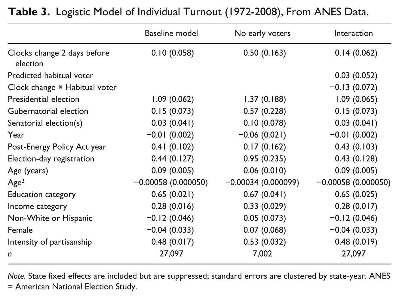
Note. State fixed effects are included but are suppressed; standard errors are clustered by state-year. ANES = American National Election Study.

The control variables mostly have plausible coefficients. Presidential elections, intense partisanship, the ability to register on the day of the election, and high levels of income or education have very large turnout-enhancing effects, whereas the coefficients on age imply turnout rates rising through most of the age distribution, only declining slightly in extreme old age. Other variables mostly do not prove to have consistently significant effect, except for a trend toward lower turnout rates over time (which may not be meaningful, given increasingly biased ANES turnout reports over time; see Burden, 2000).

One advantage of individual-level data is that they can be used to see how different groups’ turnout behavior reacts to recent clock shifts. Notably, electoral effects of a recent clock shift should, like most turnout effects, be much smaller among habitual voters who were very likely to vote even without extra time available (Aldrich, Montgomery, & Wood, 2011). Marginal voters, who need an above-average spur to turn out, may by contrast have their motivation to participate in elections more meaningfully bolstered by feeling they have a little more time on Election Day. If the causal story discussed here were really operating, in other words, the effect should be concentrated among those who are not habitual voters. Habitual voters thus offer something of a placebo test for the effects of clock shifts, a desirable cross-check of whether other observed results reflect the hypothesis rather than random chance (Sekhon, 2009).

To measure which respondents’ electoral participation was overdetermined, consider the prediction of the model from Table 3’s first column estimated without the daylight-saving-time variable. This produces an estimate of how likely each respondent would be to vote independent of the clock shift. Those with a predicted probability of voting higher than 75% are deemed habitual voters (using the predicted probability instead of the binary measure produces similar results). Interacting this measure with exposure to a recent clock shift can then be included in models predicting turnout. This checks whether habitual voters’ turnout is indeed less sensitive to recent clock shifts. This does problematically use an interactive predictor variable in a nonlinear regression (Ai & Norton, 2003), but when interpreted with due caution, the results can provide a useful sense of the relevant effects. Table 3’s rightmost column provides the model estimates.

The model tends to confirm that the end of daylight saving time matters most for those who do not habitually vote. The coefficient on recent clock shifts is positive, while that on the variable interacting clock shifts with habitual voting is negative with an almost identical magnitude. This implies that only those who are not habitual voters see an increase in expected turnout when the election comes just after the end of daylight saving time. To be specific, for someone with median levels of the other independent variables, a recent clock shift associates with a 2.6 percentage-point change in voting probability for non-habitual voters, but only a 0.2 percentage-point change for habitual voters. This tends to reinforce the evidence that daylight saving time drives the reported effects.

Conclusion: It’s About Time

Whether looking at individual survey respondents, counties in Indiana, or states within the United States, contexts where prospective voters get the benefit of an extra hour in the days just prior to an election see higher rates of turnout. The increase is comparable in magnitude with that seen by there being a gubernatorial race on the ballot, or roughly the same size as the effect seen in studies of several other forces often pointed to as shifting turnout, such as registration rules or day-of-election reminders (e.g., Dale & Strauss, 2009; Neiheisel & Burden, 2012).

This has many implications. Most directly, these concern forecasts of American elections. Turnout is not the only electoral outcome at play, as some evidence suggests that would-be Democratic voters’ turnout decisions are more sensitive to day-of-election factors (Gomez, Hansford, & Krause, 2007). The post-2006 electoral calendar may then, by more frequently boosting turnout among marginal voters, augment the performance of Democratic candidates in most years. Yet extra sleep also enhances people’s moods, which in turn associate with incumbent performance (Healy, Malhotra, & Mo, 2010). Both parties’ incumbents may then do better when elections occur just after the autumn clock shift. In other words, the conjunction of extra sleep with elections may influence not only the set of people who turn out to vote, but also the preferences of voters within that set. Furthermore, clock shifts are just one source of widespread sleep adjustments: Other events in the days before an election—whether national events like late-night games in Major League Baseball’s World Series (especially in the Eastern Time Zone), local matters like nighttime thunderstorms, or personal factors like recent cross-time-zone travel—could have similar effects.

The findings suggest several potential paths for future research. More substantively, the effects raised here may interact with other voting regulations, or with personal characteristics, that could fruitfully be considered by individual-level studies or even experimental interventions. Parents of small children, for example, may have sleep and life schedules that are relatively less attuned to the clock and so be less sensitive to the clock shifts. Indeed, evidence suggests that different personality types may respond more or less dramatically to circadian-rhythm disruptions (Suvanto, Härmä, & Laitinen, 1993). And while the American calendar may be uniquely susceptible to the effects of clock shifts, other countries might see their own specific implications. For example, in countries with endogenous election timing, governments can choose to manage turnout by strategically juxtaposing the timing of votes vis-à-vis seasonal clock changes. Even with exogenous electoral timing, politicians could manipulate sleep for electoral ends: Placing midnight phone calls to likely opposition voters shortly before an election (perhaps “accidentally”) could strategically exploit effects like those considered here. More broadly, the findings suggest that the recent vogue for biological explanations of political behavior may extend beyond genetics to matters of hormonal and other biochemical processes. The same sleep disruption that influences voting also affects other politically relevant outcomes; for instance, public opinion surveys taken just after a clock shift may also generalize less well than do those from other times. The salience of sleep is likely to expand as social trends lead to increasingly common chronic sleep deprivation (Rajaratnam & Arendt, 2001). The start and end of daylight saving time offer a small window on larger vistas of potential effects on behavior.

The results also speak to the possibilities of considering the political consequences of seemingly irrelevant policies. The arguments regarding changes in the end of daylight saving time in the United States essentially ignored elections; the debates in Congress showed more attention to evening hours of daylight trick-or-treating at Halloween. Yet precisely because the change did not explicitly aim to manipulate voting, it sheds a unique light on the public’s decision-making process surrounding voting. Other policies have similar potential. Districts vary in the length of their school day, and education advocates have long lobbied for more hours in school (Patall, Cooper, & Allen, 2010): Would this, by providing extra childcare time for parents, encourage voting among those with school-age children? Transportation policies that reduce congestion can not only free up time but also make the experience of commuting to polls less unpleasant (Eliasson, Hultkrantz, Nerhagen, & Rosqvist, 2009): Might this alter voting behavior? Overtly electoral policies certainly have important implications for political outcomes, but other regulations can also be telling.

Footnotes

Acknowledgements

I thank Amy Erica Smith, David A. M. Peterson, Brian Gaines, and the anonymous reviewers for helpful comments on earlier drafts of this article.

Declaration of Conflicting Interests

The author(s) declared no potential conflicts of interest with respect to the research, authorship, and/or publication of this article.

Funding

The author(s) received no financial support for the research, authorship, and/or publication of this article.

Notes

Author Biography

R. Urbatsch is an associate professor at Iowa State University. His research focuses on geography and political economy.

References

Norton

E. C.

(2003). Interaction terms in logit and probit models. Economics Letters, 80, 123-129.

Aldrich

J. H.

Montgomery

J. M.

Wood

(2011). Turnout as a habit. Political Behavior, 33, 535-563.

Barnes

C. M.

Wagner

D. T.

(2009). Changing to daylight saving time cuts into sleep and increases workplace injuries. Journal of Applied Psychology, 94, 1305-1317.

Burden

B. C.

(2000). Voter turnout and the National Election Studies. Political Analysis, 8, 389-398.

Dale

Strauss

(2009). Don’t forget to vote: Text message reminders as a mobilization tool. American Journal of Political Science, 53, 787-804.

Eliasson

Hultkrantz

Nerhagen

Rosqvist

L. S.

(2009). The Stockholm congestion-charging trial 2006: Overview of effects. Transportation Research Part A: Policy and Practice, 43, 240-250.

Gibson

Kim

Stillman

Boe-Gibson

(2013). Time to vote? Public Choice, 156, 517-536.

Gimpel

J. G.

Schuknecht

J. E.

(2003). Political participation and the accessibility of the ballot box. Political Geography, 22, 471-488.

Gomez

B. T.

Hansford

T. G.

Krause

G. A.

(2007). The Republicans should pray for rain: Weather, turnout, and voting in US presidential elections. Journal of Politics, 69, 649-663.

10.

Healy

A. J.

Malhotra

C. H.

(2010). Irrelevant events affect voters’ evaluations of government performance. Proceedings of the National Academy of Sciences, 107, 12804-12809.

11.

Janszky

Ljung

(2008). Shifts to and from daylight saving time and incidence of myocardial infarction. New England Journal of Medicine, 359, 1966-1968.

12.

Kamstra

M. J.

Kramer

L. A.

Levi

M. D.

(2010). Effects of daylight-saving time changes on stock market volatility: A comment. Psychological Reports, 107, 877-887.

13.

Kantermann

Juda

Merrow

Roenneberg

(2007). The human circadian clock’s seasonal adjustment is disrupted by daylight saving time. Current Biology, 17, 1996-2000.

14.

Karp

J. A.

Brockington

(2005). Social desirability and response validity: A comparative analysis of overreporting voter turnout in five countries. Journal of Politics, 67, 825-840.

15.

Kotchen

M. J.

Grant

L. E.

(2011). Does daylight saving time save energy? Evidence from a natural experiment in Indiana. Review of Economics and Statistics, 93, 1172-1185.

16.

Lahti

T. A.

Haukka

Lönnqvist

Partonen

(2008). Daylight saving time transitions and hospital treatments due to accidents or manic episodes. BMC Public Health, 8, 74.

17.

Lahti

T. A.

Leppämäki

Lönnqvist

Partonen

(2006). Transition to daylight saving time reduces sleep duration plus sleep efficiency of the deprived sleep. Neuroscience Letters, 406, 174-177.

18.

Lavie

(2001). Sleep-wake as a biological rhythm. Annual Review of Psychology, 52, 277-303.

19.

McDonald

M. P.

(2002). The turnout rate among eligible voters for U.S. States, 1980-2000. State Politics & Policy Quarterly, 2, 199-212.

20.

Michelson

(2011). Sleep time: Media hype vs. diary data. Social Indicators Research, 101, 275-280.

21.

Mills

J. N.

(1966). Human circadian rhythms. Physiological Reviews, 46, 128-171.

22.

Monk

T. H.

Aplin

L. C.

(1980). Spring and autumn daylight saving time changes: Studies of adjustment in sleep timings, mood, and efficiency. Ergonomics, 23, 167-178.

23.

Neiheisel

J. R.

Burden

B. C.

(2012). The impact of election-day registration on voter turnout and election outcomes. American Politics Research, 40, 636-664.

24.

Ohayon

M. M.

Smolensky

M. H.

Roth

(2010). Consequences of shiftworking on sleep duration, sleepiness, and sleep attacks. Chronobiology International, 27, 575-589.

25.

Olsen

O. K.

Pallesen

Eid

(2010). The impact of partial sleep deprivation on moral reasoning in military officers. Sleep, 33, 1086-1090.

26.

Patall

E. A.

Cooper

Allen

A. B.

(2010). Extending the school day or school year: A systematic review of research (1985-2009). Review of Educational Research, 80, 401-436.

27.

Pilcher

J. J.

Huffcutt

A. I.

(1996). Effects of sleep deprivation on performance: A meta-analysis. Sleep, 19, 318-326.

28.

Rajaratnam

S. M. W.

Arendt

(2001). Health in a 24-hour society. Lancet, 358, 999-1005.

29.

Rallings

Thrasher

Borisyuk

(2003). Seasonal factors, voter fatigue and the costs of voting. Electoral Studies, 22, 65-79.

30.

Sadavoy

(1997). Survivors: A review of the late-life effects of prior psychological trauma. American Journal of Geriatric Psychiatry, 5, 287-301.

31.

Schredl

Piel

(2006). War-related dream themes in Germany from 1956 to 2000. Political Psychology, 27, 299-307.

32.

Sekhon

J. S.

(2009). Opiates for the matches: Matching methods for causal inference. Annual Review of Political Science, 12, 487-508.

33.

Shipan

C. R.

(1996). Senate committees and turf: Do jurisdictions matter? Political Research Quarterly, 49, 177-189.

34.

Suvanto

Härmä

Laitinen

J. T.

(1993). The prediction of the adaptation of circadian rhythms to rapid time zone changes. Ergonomics, 36, 111-116.

35.

Valdez

Ramírez

García

(2003). adjustment of the sleep-wake cycle to small (1-2 h) changes in schedule. Biological Rhythm Research, 34, 145-155.

36.

Wagner

D. T.

Barnes

C. M.

Lim

V. K. G.

Ferris

D. L.

(2012). Lost sleep and cyberloafing: Evidence from the laboratory and a daylight saving time quasi-experiment. Journal of Applied Psychology, 97, 1068-1076.