Candidate Age and Youth Voter Turnout

Abstract

The research addresses youth voter turnout in the United States and, specifically, tests the relationship between candidate age and a commitment to vote by young people in a controlled experiment. We learn that potential young voters are more willing to commit to vote when they view pictures of younger candidates running. This is the case after controlling for the age and partisanship of respondents. In a real-world test of our experimental results, we examine state-level variation in youth voter turnout in midterm governor and Senate races (1994-2010). In the state-level analysis, we find a larger candidate age gap in governor and Senate races associates with higher levels of youth mobilization. In all, the research affirms the value of candidate characteristics as a predictor of voting behavior.

Keywords

youth mobilization voter turnout candidate age social identity theory

. . . non-voting among the young seems more important than non-voting among the very old for the practical reason that it seems more remediable.

—Converse (1971, p. 445)

This research addresses the extent to which the age of candidates influences youth voter mobilization. The broadest normative focus is a concern for widespread participation in democracies to foster republican accountability (see Cohen, 1973; Pennock, 1979). The more specialized motivation is a more complete understanding of overall low levels of youth voter turnout in the United States. This specific question has been a concern of scholars for some time, evidenced by Converse’s (1971) work, which draws data from elections held in the 1950s. Intriguingly, Converse’s work on youth voter turnout predates passage of the Twenty-Sixth Amendment in 1971, which lowered the eligible voting age from 21 to 18 years, and led to an even greater disparity in turnout between the young and other age cohorts (Burden, 2000).

Figure 1 demonstrates lower youth voter participation rates in U.S. national elections, since 1978.¹ From the figure, we learn the phenomenon of lower youth voter turnout has persisted into the 21st century. Empirically the gap in voter turnout between the youngest and oldest age groups has averaged around 33% since the late 1970s (33.9% from 1978 to 2000 and 33.6% from 2002 to 2010). The largest disparity in voter turnout between the youngest and oldest age cohorts occurred just prior to the dawn of the 21st century in the 1998 midterm elections (44.1%). However, there is a second trend of interest in Figure 1 that is not obvious at first. Note less variation in the line representing voter turnout of the age group most likely to vote (65 and older). This compares to a line with comparatively more movement for 18- to 24-year-olds. The standard deviation of the 18 turnout values representing the group ages 65 and older is 4.8%, whereas the standard deviation of youth voter turnout is 10.8%. This extra volatility in aggregate youth voting suggests there may be factors in play that influence youth voter turnout that do not affect other age groups (standard deviation of all age groups equals 7.7%). This research begins to unravel whether the age of candidates may be part of an explanation for the greater variability in youth voter turnout.

Figure 1.

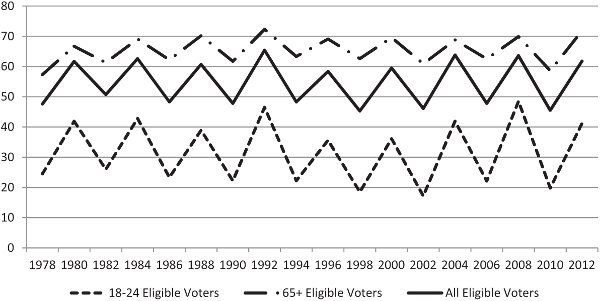
Voter turnout in U.S. national elections: 1978-2012.

Electoral participation is ranked high by those who seek to define and describe quality democracy (Dahl, 1971; Powell, 1982) and many recognize that political elites have less concern for the policy preferences of non-voters (Almond & Verba, 1963; Berelson, 1952). Although some suggest non-voters and voters do not differ appreciably, Arend Lijphart (1997) in his presidential address to the American Political Science Association challenged this contention, suggesting that if mobilized the class consciousness of non-voters would increase and their opinions would change. William Riker (1965) for his part argues, “the essential democratic institution is the ballot box” (p. 25), and therein lies democratic accountability. Others suggest, specifically, “because electoral engagement is an essential element of a strong democratic system, youth disengagement harms the nation as a whole” (Ulbig & Waggener, 2011, p. 544; see also Arendt, 1958; Barber, 1984; Lijphart, 1997; Pateman, 1970). If young adults turn out to vote at a higher rate, arguably, initiatives and policies that address their particular policy concerns would become more salient.

Against the normative backdrop of quality representation born of higher youth voter turnout, this research uses elements of social identity theory (SIT), which has been tapped to explain the electoral behavior of Latin Americans (Jackson, 2011), African Americans (Bobo & Gilliam, 1990), women (Dolan, 1998; Matson & Fine, 2006), and individuals of a generic identity (Bassi, Morton, & Williams, 2011). Specifically, SIT suggests people will vote for and support candidates who are like themselves or are members of the same group (Conover, 1984; Greene, 1999; Huddy, 2001; Oakes, 2002; Tajfel, Billig, Bundy, & Flamet, 1971). Groups can be defined as individuals with like demographic characteristics, individuals with similar views, or simply people who belong to the same organization. Here, we use the logic of SIT to theorize that potential young voters will be more likely to identify with younger candidates and this increased connectivity will cause greater electoral mobilization. Traditionally, identities examined through the lens of SIT are static, yet age is fluid. However, we feel age can work as an “identity” and a rallying agent similar to race and gender empathy. We suspect this might especially be the case when there is considerable disparity in the age of candidates.

At the heart of this research is a controlled experiment that isolates the influence of candidate age on a commitment to vote by young adults. Specifically, college students in general education classes at a midsized, public, Midwestern university were asked to report their likelihood of voting after viewing pictures of older and younger looking candidates in hypothetical elections. To deal with possible imbalance across randomly constituted groups in the statistical tests which follow, we control for the age and partisanship of the students. We also use two sets of pictures to help address the possibility that a particular set of candidate photographs is driving the results.² In the end, we learn traditional college students are more likely to commit to vote when younger looking candidates are running.

There has been long-standing academic uneasiness about external validity when using college students in social science experiments. In this instance, the concern is whether college students between the ages of 18 and 24 accurately represent the population of others the same age who have not attended college. In our case, we think the bias may function in a manner that would cause us to underreport evidence of SIT. One might imagine students in college being more politically sophisticated, on average, than those not enrolled in college and consequently less likely to use a simple heuristic such as candidate age to determine whether they would turn out to vote. If this were the case, our results might prompt Type II error or the tendency to accept a null hypothesis when the reality is that a relationship exists. Importantly, recent research argues that external and internal validity are not necessarily compromised by student participants (Druckman & Kam, 2011).³ Druckman and Kam (2011), using simulations, suggest student participants do not pose an appreciably greater “treatment effect” than do other less homogeneous participants (p. 50).

To provide a real-world test of our experimental findings, we examine state-level variation in youth voter turnout in midterm gubernatorial and Senate elections in the American states. The focus is on midterm elections to prevent the age of the more highly visible U.S. presidential candidates from tainting the analysis. As gubernatorial and Senate candidates are often both over 50 years of age and there is a real dearth of races with a young candidate running, we focus on the candidate age gap while controlling for the youngest candidate running. But first, we scrutinize carefully four Senate races, which had a candidate less than 35 years of age. In these races, we uncover empirical evidence in support of SIT. In the systematic test of the candidate age gap, we learn 18- to 24-year-olds voted at a statistically higher rate in elections when the age difference between candidates was larger, although the effect is only present in reasonably competitive races.

Explaining Youth Voter Turnout

In much of the voting turnout literature, it is widely recognized that as one gets older, participation rates go up, but gradually fall off very late in life (Brown, Jackson, & Wright, 1999; Campbell, Converse, Miller, & Stokes, 1960; Converse, 1971; R. E. Wolfinger & Hoffman, 2001; N. H. Wolfinger & Wolfinger, 2008; for generational effects on voter turnout, see Lyons & Alexander, 2000). Voter registration requirements are believed to be one of the culprits (Converse, 1971) because of the burden they place on first-time voters, wary of the rational calculus or costs associated with voting (Blais, 2000). Converse (1971) uncovers a particular burden placed on young voters by voter registration laws that require individuals to register to vote “at some other time than Election Day itself” (p. 466; see also Kaufmann, Petrocik, & Shaw, 2008, p. 118). In the experiment conducted for this research, voter registration requirements are held constant by conducting the test in a single geographic location, and also by the fact students are asked to respond to questions about a hypothetical election. In the real-world test of the age gap, a control variable for same day voter registration is incorporated in the model.

In addition, it is well-established that education (Milligan, Moretti, & Oreopoulos, 2004) influences individual and aggregate youth voter turnout levels (Jackman, 1987; Powell, 1986). A primary concern has been age variation in political knowledge (Delli Carpini & Keeter, 1991; Galston, 2004; Jennings, 1996).⁴ In this vein, Cogan (1997) and Eagles and Davidson (2001) suggest the declining value of high school civics classes may be the causal mechanism. Others note the reduced time young people spend reading newspapers (Wattenberg, 2012). In the experiment, we hold education constant via random assignment of college students, in general education classes to two different treatment groups and a control group. In the gubernatorial and Senate race analysis, we use the turnout of eligible voters 25 and older, in each state and each election year, as a means of controlling for the long list of systematic and random factors that influence state-level and year-specific voter turnout values.

Another species of research on youth voter turnout focuses on electoral conditions where individuals live (Cho, Gimpel, & Dyck, 2006; Fauvelle-Aymar & Francois, 2006; Gimpel, Dyck, & Shaw, 2004; Kenny, 1992; Pacheco, 2008; Pacheco & Plutzer, 2008). For example, Pacheco (2008) finds the amount of electoral competition in a geographic region has a positive effect on voter turnout. Others note that electoral competition increases voter turnout in both high-profile (Kau & Rubin, 1976) and second-order elections (Barzel & Silberberg, 1973; Patterson & Caldeira, 1983). In the experiment, we control for a competitive electoral environment by conducting the test in a single geographic location.

Next, scholars have come to appreciate the manner by which economic conditions influence voter turnout (Rosenstone, 1982; Stevens, 2006). Specifically, unemployment (Grant & Toma, 2008; Southwell, 1988) is believed to affect voting rates. In an experiment, Lassen (2005) finds both public and private employment inversely relate to voter turnout. By extension, unemployment should associate positively with more voting.⁵ In the experiment, unemployment will be held constant by random assignment to test groups. In the analysis of gubernatorial and Senate races, we control for the October unemployment rate in each state preceding each election.⁶ We suspect that unemployment may have a special influence on the mobilization of young Americans who may be looking for their first job after finishing either high school or college.

With all the work just cited on voter turnout, generally, and youth voter turnout, specifically, one might wonder why yet another exposé on the subject matter. The unique contribution this research seeks to make is a test of youth voter mobilization as it relates to candidate age, a variable that has received comparatively less scholarly attention.

An Experimental Test of Youth’s Commitment to Vote and Candidate Age

Researchers have found candidate appearance plays a role in citizen evaluations (Banducci, Karp, Thrasher, & Rallings, 2008). To test whether a young looking candidate will lead young people to commit to vote at a higher rate, we build on the work of Sigelman and Sigelman (1982) who expose undergraduate students to written descriptions of fictional political candidates of different ages, gender, and race. The Sigelmans uphold a “similarity hypothesis” (Sigelman & Sigelman, 1982, p. 267), and suggest there is “ageism” in America’s youth, or that young voters are prejudiced against older candidates. Our research differs considerably from the Sigelmans’ work because our concern is a commitment to vote rather than vote choice. Consistent with Banducci et al. (2008), but distinct from the Sigelmans, we use photographs to answer our research question.⁷

In the analysis that follows, we test respondents’ commitment to vote in a race with two old candidates running, a race with one old and one young candidate running, and a race with two young candidates. A total of 784 students participated in the experiment, but we eliminate incomplete surveys and responses by students 25 years of age or older. We had no respondents less than 18 years of age. We exclude the older group for the sake of being consistent with the age designation (18-24) most commonly used by the Census Bureau and other investigators of youth voter mobilization. This yields a useable sample of 691, representing 88% of participants. Approximately one third of the students saw each of the three pairs of photographs.⁸ The experiment took place in general education or freshman-level courses over three semesters. Students were told they were involved in research on candidate image.

All photos were of White males to control for possible racial and gender effects on a commitment to vote.⁹ The experiment used two sets of six photographs to control for the possibility that a particular set of photographs was driving the results and we control for the 1st Set of Pictures in the model that follows and expect a commitment to vote to be lower with the first set of pictures because a post hoc analysis determined that the second set of photographs depicted older candidates who “looked older.” As a screen for our true test, students were asked which candidate they would be more likely to vote for,¹⁰ and then, their likelihood of voting in each race on a scale ranging from “1” to “10,” with 10 representing the strongest commitment to vote. The appendix exhibits the form students were asked to fill out.

Table 1 provides summary data on the dependent variable and explanatory variables used in the experiment. Concerning the dependent consideration, Commitment to Vote, the sample returned a mean value of 6.03 with a one standard deviation of 2.55 points. Concerning our treatment—photos of candidates of varying age—we use the hypothetical race with two older looking candidates running as our reference group. Hence, we have a variable for Old vs. Young and a second variable for Young vs. Young. Our expectation is that there will be a stronger commitment to vote when there is at least one young candidate running and the strongest commitment to vote when there are two young candidates running.

Table 1.

Summary Data Youth Commitment to Vote Experiment.

Dependent variable	Minimum value	Maximum value	Mean	SD
Commitment to vote	1	10	6.03	2.55
Treatment variables
			Frequency
Old vs. young	0	1	230/691
Young vs. young	0	1	218/691
Control variables
1st set of pictures	0	1	201/691
			Mean	SD
Participant age	18.00	24.83	20.27	1.58
			Frequency
Strong Republican	0	1	16/691
Republican	0	1	104/691
Indep Leaning Republican	0	1	72/691
Independent	0	1	132/691
Indep Leaning Democrat	0	1	148/691
Democrat	0	1	174/691
Strong Democrat	0	1	45/691
N		691

Note. Indep. = Independent

We begin with a simple bivariate test of the association between a commitment to vote and the two treatment groups and the control group. Table 2 displays these results. There is a statistically insignificant positive relationship between a commitment to vote and the set of photographs that depicted one old and one young candidate running. There is a statistically significant and positive bivariate relationship between a commitment to vote and the set of pictures that exhibited two young candidates facing off. Third, there is a significant negative relationship when considering a hypothetical race with two older looking candidates running.

Table 2.

Bivariate Relationships Between a Commitment to Vote and Different Groups.

	Expected sign	Pearson’s r, p value	Sample size
Treatment groups
Old vs. young	+	.02, p < .35	230
Young vs. young	+	.07, p < .03	218
Control group
Old vs. old	−	−.09, p < .02	243

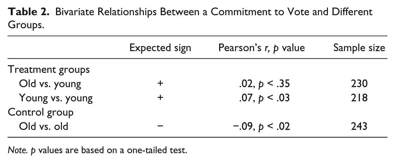
Note. p values are based on a one-tailed test.

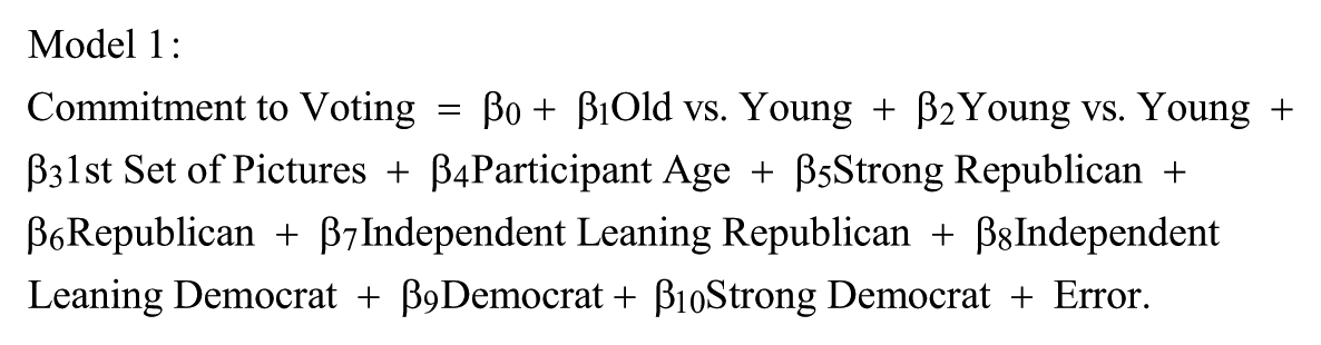
We now turn to a regression analysis that will control for the set of pictures used, but also Participant Age and a list of party identifications. The logic of random assignment in an experiment suggests this may be unnecessary; however, a regression with theoretically important control variables included ought to sharpen the estimates. Participant age we hold will be positively associated with a commitment to vote (Mean age = 20.27; 1 SD = 1.58). We measured party identification using the traditional seven ordered categories—but not the multi-stage question sequence—from the American National Election Study (see the appendix). Our expectation is that self-identified Independents will be less likely to commit to vote (Keith et al., 1992) and use them as our omitted category. Hence, we expect the tests of Strong Republican, Republican, Independent Leaning Republican, Independent Leaning Democrat, Democrat, and Strong Democrat will all return positive coefficients. We suspect Strong Party Identifiers will be especially more likely to commit to vote (Abramson & Aldrich, 1982; Campbell et al., 1960). In addition, some prior work has found that Republicans have higher turnout rates (Conway, 1985; Mangum, 2003). We estimate the following ordinary least squares (OLS) model and report the results in Table 3:

\begin{array}{l} Model 1 : Commitment to Voting = β_{0} + β_{1} Old vs . Young + β_{2} Young vs . Young + β_{3} 1 st Set of \\ Pictures + β_{4} Participant Age + β_{5} Strong Republican + β_{6} Republican + β_{7} Independent Leaning \\ Republican + β_{8} Independent Leaning Democrat + β_{9} Democrat + β_{10} Strong Democrat + Error \end{array} .

Table 3.

Youth Commitment to Vote and Young Candidates: An Experiment (Model 1: Ordinary Least Squares Regression).

	Expected sign	Coefficient (SE)
Treatment variables
Old vs. young	+	0.45 (0.22)*
Young vs. young	+	0.61 (0.23)**
(Old vs. old omitted group)
Control variables
1st set of pictures	−	−1.14 (0.21)***
Participant age	+	0.03 (0.06)
Strong Republican	+	0.89 (0.64)
Republican	+	1.77 (0.32)***
Independent Leaning Republican	+	1.56 (0.36)***
Independent Leaning Democrat	+	1.31 (0.29)***
Democrat	+	0.09 (0.29)
Strong Democrat	+	0.99 (0.42)**
(Independents omitted group)
Constant		4.66 (1.27)***
F statistic		8.87***
Adjusted R²		.10
Sample size		691

p < .05. **p < .01. ***p < .001 (one-tailed tests).

First, and foremost, we learn from model output that when there is a young candidate running there is a stronger commitment to vote on the part of student participants, all else being equal. Moreover, based on the size of the coefficients and the level of statistical significance, the greatest commitment to vote occurs when there are two young looking candidates running. This is consistent with our hypotheses and the logic of SIT.

Considering the control variables, we learn the first set of pictures used is linked to a weaker commitment to vote as anticipated and that participant age, on average, is positively associated with a commitment to vote, but the test does not return a statistically significant coefficient. Minimal variation on the age variable undoubtedly contributes to the lack of a statistical relationship. Last, several of our partisan hypotheses are confirmed. We find that strong Democratic Party identifiers are more likely to commit to vote, on average, but the same is not true for strong Republican Party identifiers. The small number of strong Republican Party identifiers in our sample (16 out of 691) may be compromising the estimate derived from this test. Other Republicans are more committed to vote as anticipated and it is the case, across the board, that Independents are the least likely to commit to vote, on average.

We also estimate the model as an ordered logit to substantiate our findings and to gain some insights into the substantive significance of our tests. With the ordered logit regression, we again use the 1 to 10 scale representing a commitment to vote. These results are not reported in any table, but are available in the online appendix. Importantly, the tests of statistical significance are consistent with the OLS model output. Moreover, we learn the odds of moving from one value of the dependent variable (a commitment to vote) to the next value in a positive direction are 1.37 times greater when there is one young candidate running. This grows to 1.56 times greater when there are two young candidates running, ceteris paribus. The odds of moving up one value on the scale are 3.87 times greater if the student is a Republican and 2.40 times more likely when the respondent is a Strong Democrat.

Looking for Evidence of SIT in Cross-State Variation in Youth Voter Turnout

The experimental results affirm the potential value of SIT as it relates to candidate age. Next, we turn to an analysis of some real-world election scenarios to see if there is any evidence of SIT in some recent high-profile American elections. Specifically, we look for variation in youth voter turnout when there are young candidates running for either a U.S. Senate seat or in governor races during the five most recent midterm election cycles (1994, 1998, 2002, 2006, and 2010). We focus our attention on variation in voter turnout of the voting eligible population from the 18- to 24-year age group, as measured by the Current Population Survey and reported by the U.S. Census Bureau. We construct an original data set that includes all gubernatorial and Senate races in the five election cycles. In some state-election years, there are races for both governor and Senate occurring, concurrently. When this happens, we consider the age of four candidates representing the two highest vote getters in the two races. In the end, we examine 230 elections, 50 standalone Senate races, 63 standalone gubernatorial elections, and 117 elections where there is both a governor and Senate race on the same ballot.¹¹

Most specifically, we collect data on two unique considerations of candidate age. We measure the age of the Youngest Candidate and the Candidate Age Gap.¹² We always use the age of the two candidates who finished first and second, nearly always one Republican and one Democratic Party candidate. In standalone gubernatorial and Senate elections, the measurement is straightforward. For the elections, where there were concurrent gubernatorial and Senate races, we use the age of the youngest of the four candidates to capture “Youngest Candidate.” For the age gap consideration, we use the difference between the oldest and youngest candidate among the four candidates running.

We note upfront that of the 698 individuals we study, there are only four candidates under the age of 35, all of them Senate candidates. The average age of the youngest candidate is 48.0 years. This creates a considerable obstacle for any test of SIT using data from these races. Yet, systematic analysis of a relationship between candidate age and youth voter turnout in more local elections, where younger candidates might be present, is compromised by long ballots and the lack of youth voter turnout estimates at appropriate geographic aggregations. We forge forward with a test of SIT using the age of candidates at the top of midterm election ballots. Table 4 exhibits youth voter turnout figures in the four cases with Senate candidates under 35 years of age and compares this with youth voter turnout in the previous midterm election and to the voter turnout of people 25 and older in these same elections.¹³ We expect there to be a smaller voter turnout gap between the two age groups (18-24 and 25+) when there is a young candidate running. Put differently, evidence of SIT, based on age, will be present if voter turnout of young people more closely mirrors the turnout of others when a candidate under the age of 35 is running.

Table 4.

Youth Voter Turnout Compared With Other Ages and Previous Election: Young Candidate Running.

Year	State	Youngest age^a		18- to 24-year-old TO	25+ year old TO	TO gap
2002	Michigan	33.8	Young candidate running	21.5	54.7	33.2
2002	Michigan	33.8	Previous midterm election	18.1	56.1	38.0
2010	Arizona	32.4	Young candidate running	27.1	52.0	24.9
2010	Arizona	32.4	Previous midterm election	17.5	50.5	33.0
2010	Illinois	34.6	Young candidate running	20.6	49.5	28.9
2010	Illinois	34.6	Previous midterm election	20.8	51.3	30.5
2010	South Carolina	33.2	Young candidate running	33.5	53.2	19.7
2010	South Carolina	33.2	Previous midterm election	18.6	49.0	30.4

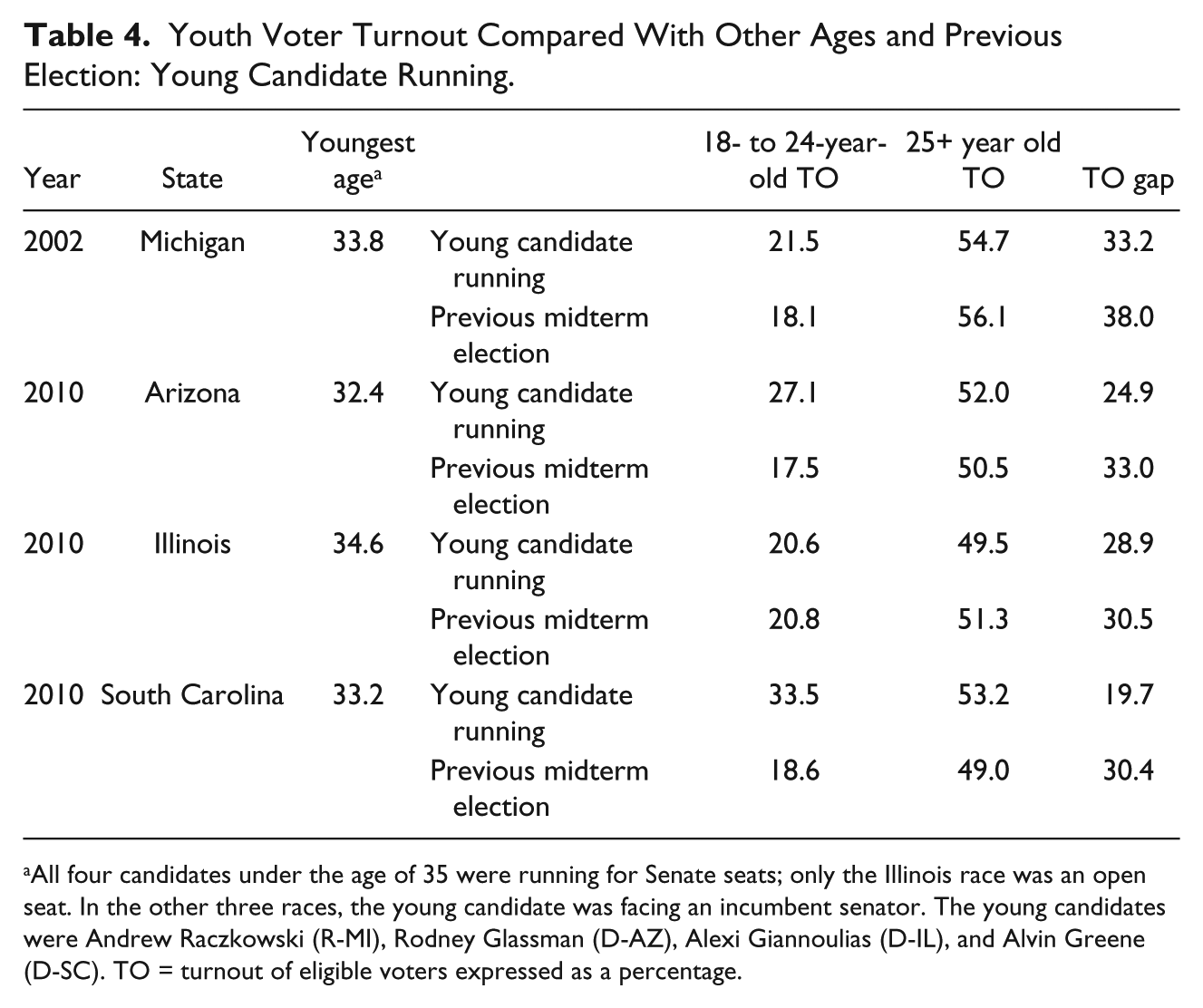
All four candidates under the age of 35 were running for Senate seats; only the Illinois race was an open seat. In the other three races, the young candidate was facing an incumbent senator. The young candidates were Andrew Raczkowski (R-MI), Rodney Glassman (D-AZ), Alexi Giannoulias (D-IL), and Alvin Greene (D-SC). TO = turnout of eligible voters expressed as a percentage.

By examining column 5 in Table 4, we note that in three of the four cases, voter turnout for the young age group is higher than it had been in the previous midterm election, when there was not a candidate under the age of 35 in the running—nearly 15 percentage points higher in South Carolina. In the one instance, where voter turnout was not higher, the under 35 candidate in Illinois was running in an open seat race against a relatively young Mark Kirk (R-IL), 51 years of age at the time of the election. The candidate age gap would have been less obvious in this race than it was in the other three races, which had a younger candidate facing off against incumbent senators who were 59, 68, and 74 years of age. Yet, in all four instances (see column 7), the difference between the two age groups drew closer when a candidate under 35 was running. In Illinois, where young people did not turn out at a higher rate, compared with the previous election, the difference with the other age group in 2010 was still smaller than it had been in 2006.

Given so few instances of young candidates running, we turn to an analysis of the candidate age gap. Arguably, the presence of a “younger” candidate becomes more obvious when he or she is juxtaposed in a race with a considerably older candidate. In the experiment when respondents saw pictures of one young and one old candidate running, they were more likely to commit to vote than when they saw pictures of two old candidates; albeit the commitment to vote was not as strong as it was when viewing two young candidates. We know in the 2008 American presidential race, which saw the largest age gap between presidential candidates since the Twenty-Sixth Amendment was passed (Barack Obama was 25 years younger than John McCain), eligible 18- to 24-year-olds turned out at the highest rate (48.5%) they had since the seminal presidential election post–Twenty-Sixth Amendment.¹⁴ In contrast, the smallest age gap between presidential candidates, in the past four decades, occurred in 2000 when George W. Bush faced Albert Gore (a 2-year gap). In this instance, the turnout of eligible 18- to 24-year-olds was the second lowest it has been (35.6%) during recent presidential election years.¹⁵

Given observed anecdotes and the results of our experiment, our suspicion is that the candidate age gap can be a motivating factor bringing young people to the polls in gubernatorial and Senate races. Specifically, we hypothesize that as the difference in candidate age grows, eligible voters between 18 and 24 years of age, in the aggregate, will be more likely to turn out to vote. Importantly, we know the candidate age gap has no relationship with voter turnout of the eligible population 25 and older. In the five elections cycles we examine, the bivariate correlation between Voter Turnout 25+ and the candidate age gap is insignificant and actually negative (r = −.06, p < .38). If we are able to uncover a significant positive association between the age gap and youth voter turnout, this will be occurring independent of any influence the age gap has on voter turnout of older voters.

In the analysis of the effect of candidate age gap on youth voter turnout, we will include in the model voter turnout of those 25 and older. There is no causal argument here; instead the inclusion of voter turnout of non-youths is intended as a surrogate for the myriad of systematic and random factors that can influence voter turnout across all ages. Not the least of these is state-level electoral competition (Durden & Gaynor, 1987; Tucker, 1986). Note 16 provides a list of bivariate correlations between factors others note influence voter turnout and turnout of the 25 and older population during the time period of this study.¹⁶

We do include two additional considerations that we believe will have a disproportionate influence on youth voter turnout, specifically. We include the October Unemployment Rate and whether a state at the time the election was held allowed Same Day Voter Registration.¹⁷ Unemployment is negatively correlated with voter turnout of eligible voters 25 and older (r = −.18, p < .006); however, we hypothesize it will produce a positive association with youth voter turnout.¹⁸ Our hunch is that, in the aggregate, young people will be frustrated by the lack of job prospects and will consequently be more inclined to show themselves at the polls when state unemployment is higher. Next, scholars note residential mobility decreases voter turnout rates (Highton, 2000), and higher levels of residential mobility among young Americans cause us to control for same day voter registration, which was allowed in eight states for at least some of the time period analyzed.

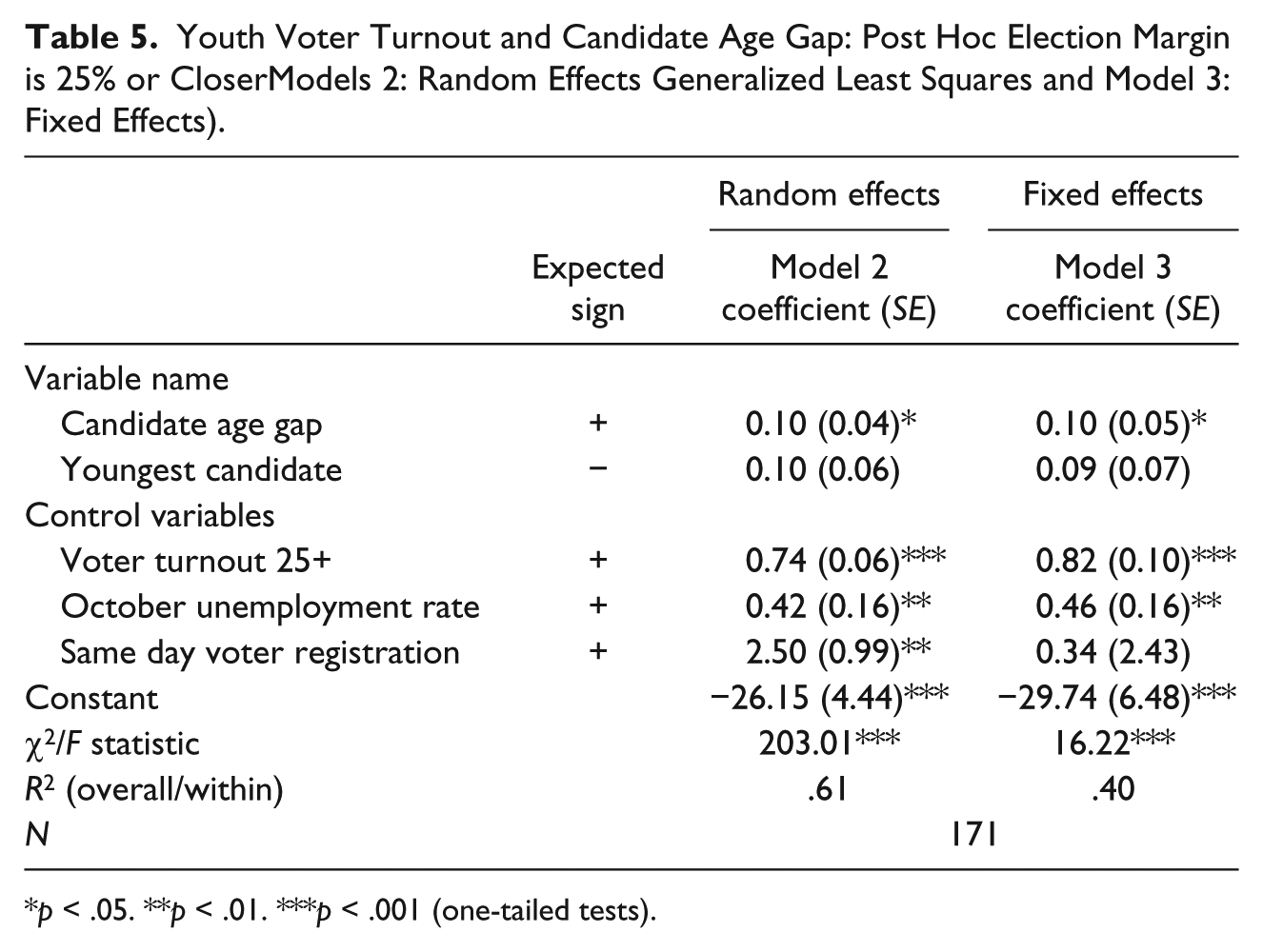
Table 5 reports the results of the candidate age gap test. The sample size drops from 230 to 171 because we eliminate races where the winning candidate had over a 25% margin of victory. The 171 cases include 51 standalone gubernatorial races, 31 standalone Senate races, and 89 races when there was both a gubernatorial and Senate race on the same ballot. It is important to point out that when we estimate the models using all 230 cases, we cannot reject the null hypothesis that the candidate age gap has no influence on youth voter turnout. However, it is difficult to imagine the age of candidates influencing voter turnout rates when there is little electoral competition or expectation that one’s vote will make a difference.¹⁹

Table 5.

Youth Voter Turnout and Candidate Age Gap: Post Hoc Election Margin is 25% or CloserModels 2: Random Effects Generalized Least Squares and Model 3: Fixed Effects).

	Expected sign	Random effects	Fixed effects
	Expected sign	Model 2 coefficient (SE)	Model 3 coefficient (SE)
Variable name
Candidate age gap	+	0.10 (0.04)*	0.10 (0.05)*
Youngest candidate	−	0.10 (0.06)	0.09 (0.07)
Control variables
Voter turnout 25+	+	0.74 (0.06)***	0.82 (0.10)***
October unemployment rate	+	0.42 (0.16)**	0.46 (0.16)**
Same day voter registration	+	2.50 (0.99)**	0.34 (2.43)
Constant		−26.15 (4.44)***	−29.74 (6.48)***
χ²/F statistic		203.01***	16.22***
R² (overall/within)		.61	.40
N		171

p < .05. **p < .01. ***p < .001 (one-tailed tests).

Because our data are arrayed over time and across the same 50 states, there is the possibility that values on the dependent variable may be correlated with one another in a manner that unexplained variance (or error) is not random. For this reason, we adopt a random effects generalized least squares (GLS) model specification. We also estimate a fixed effects model to test whether our age variables have an influence on youth voter turnout within each of the 50 states.²⁰

We test the following two models:

\begin{array}{l} Model 2 (Random Effects) : {Youth Voter Turnout}_{i t} = β_{0} + β_{1} {Candidate Age Gap}_{i t} + β_{2} Young \\ {Candidate}_{i t} + β_{3} {October Unemployment Rate}_{i t} + β_{4} {Same Day Voter Registration}_{i t} + μ_{i} + v_{i t} \end{array},

\begin{array}{l} Model 3 (Fixed Effects) : {Youth Voter Turnout}_{i t} = η_{i} + β_{1} {Candidate Age Gap}_{i t} + β_{2} Young \\ {Candidate}_{i t} + β_{3} {October Unemployment Rate}_{i t} + β_{4} {Same Day Voter Registration}_{i t} + μ_{i t} \end{array},

where i indexes the American states and t indicates each of the five midterm elections analyzed (1994, 1998, 2002, 2006, and 2010).

When we truncate the analysis and look at just those races that, in the end, were reasonably competitive, we can report the candidate age gap is statistically linked to higher youth voter turnout.²¹ The substantive significance, although not dramatic, is potentially important. Considering the age gap and the random effects model (Model 2), our results suggest an increase in 1 year in the candidate age gap associates with about a 0.10% increase in youth voter turnout, on average. Put differently, an increase in the candidate age gap of 30 years (e.g., one candidate is 35 and the other is 65 years of age) ought to increase youth voter turnout by about 3%, ceteris paribus. The average age gap for cases in this analysis is 13.9 years, with a minimum age difference of 0.2 years and a maximum of 41.8 years. The youngest candidate variable does not produce a statistically significant association with youth voter turnout after controlling for the age gap and other factors.

Considering voter turnout of the 25 and older population and the two control variables, the former is linked in a statistically important manner to youth voting. We know that overall voter turnout is determined by a whole host of, often times random, state-year circumstances and we hope that these are being captured by the Voter Turnout 25+ consideration. The two control variables both perform as hypothesized. The October unemployment rate serves to mobilize younger voters both over time and between states (Model 2) and within states (Model 3). Considering Model 2, we learn that a 1% increase in the October unemployment rate associates with a little less than a half percentage point increase (0.42) in youth voter turnout. Alternatively, a one standard deviation increase in the October unemployment rate (2.09%) across the five election cycles produces an increase in youth voter turnout of about 1%, on average. Our analysis suggests that states that allow same day voter registration can expect about a 2.5% increase in youth voter participation, on average. In the fixed effects model, however, the coefficient obtained from the test of same day voter registration is indistinguishable from zero. Limited variation within states is likely responsible for the null finding. The only within-state variation occurs as the result of three states that adopt the policy during the time period of this study (New Hampshire after 1996, Montana after 2005, and Iowa after 2007).

Conclusion

The research tests the value of SIT, experimentally, and through a follow-up analysis of some real-world election scenarios. In the first instance, the random assignment of students and a considerable sample size afford the opportunity to test an age stimulus while controlling for a whole host of considerations that might influence the likelihood that a young person would commit to vote. To tighten our estimates, we control directly for participant age and partisanship. Our results suggest a stronger commit to vote when young adults view younger looking candidates running, affirming the value of SIT as it relates to candidate age. One possible shortcoming is that our sample includes only young adults who are enrolled in college. The question is whether the results are applicable to young people who do not attend college. Further studies can answer this question. However, if we assume that more educated young adults, enrolled in college, use more information to make political decisions, and are less likely to use heuristic shortcuts, it is possible that we are actually underreporting the extent to which candidate age predicts a young adult’s commitment to vote.

When we put our experimental results to task by examining real-world election scenarios, we can easily find anecdotes from presidential and Senate races where the age gap or age of the youngest candidate appears to predict youth mobilization. Most directly, an analysis of four Senate races with a candidate under the age of 35 finds young Americans voting at higher rates or at a rate more similar to other Americans. In a systematic multivariate test of the age gap, we learn that age difference is associated with greater youth voter turnout, although only when there is some reasonable level of electoral competition. We can also note that the October unemployment rate and same day voter registration laws, on average, influence youth voter turnout in the American states in a statistically and substantively important manner.

Our results from the real-world test would benefit from a larger sample of young candidates. Perhaps an analysis of young mayoral or U.S. House candidates would be a suitable testing ground for further inquiry into SIT as it relates to candidate age. Data limitations and long ballots, however, will present obstacles that will need to be navigated. Last, we would like to point out that our real-world tests are based on an analysis of less salient midterm elections. These less noticed elections may be creating a bias that would cause one to undervalue SIT as it relates to candidate age. It may be that the candidate age considerations will have an even greater effect in more prominent presidential election cycles. The reasoning is that the more motivated voting population, in midterm elections, may be less influenced by a voting cue such as candidate age. When the young voting population grows in presidential elections, we might see the less committed pool of voters more susceptible to the use of a shortcut, such as age, to determine their presence at the polls.

Footnotes

Appendix-Experimental Instrument

This research recognizes that there is insufficient information provided to determine a vote choice. However, our interest is purely in the effect that candidate image has on voting behavior. Hence, we are going to ask you to respond to two questions using only a set of pictures to base your answers on. First, we need to know a little about you. Please answer the following questions about your background:

Date of Birth: ______ ______ _______

Month Day Year

Circle the Appropriate Category:

Party Affiliation: Strong Republican Republican Independent Leaning Republican Independent Independent Leaning Democrat Democrat Strong Democrat

Gender: Male Female

Which candidate you would you be more likely to vote for.Circle either Candidate A or Candidate B:

Candidate A Candidate B

Now, based on the photos how likely would you be to turn out to vote? Please circle a number on the scale from 1 to 10.

1 2 3 4 5 6 7 8 9 10

Definitely Definitely

would not would vote

vote

Note. Institutional Review Board exemption was granted because the research was conducted anonymously without any threat to participants. Code of Federal Regulations (45 CFR 46) 46.101b, paragraph 2 (February 1, 2012).

Acknowledgements

We would also like to extend our appreciation to Benjamin Donovan for research assistance. We would like to thank Dr. Artemus Ward, Rebecca Hannagan, and Jennifer Soss for allowing us to use their classrooms to conduct the experiment. We would also like to thank Dr. Mathew Streb and Dr. Jeffery Mondak for their feedback on issues related to research design, Dr. Brad Bishop for advice on modeling decisions, and we wish to extend a significant debt of gratitude to the anonymous reviewers and the editor of American Politics Research who provided valuable feedback on previous drafts of the article.

Authors’ Note

This research was first presented at the 2012 Midwest Political Science Association Conference.

Declaration of Conflicting Interests

The author(s) declared no potential conflicts of interest with respect to the research, authorship, and/or publication of this article.

Funding

The author(s) received no financial support for the research, authorship, and/or publication of this article.

Notes

Author Biographies

Michael J. Pomante II is a doctoral candidate in the political science department at Northern Illinois University. He is co-author, with Scot Schraufnagel, of the Historical Dictionary of the Barack Obama Administration.

Scot Schraufnagel is an associate professor of political science at Northern Illinois University. He is author of Third Party Blues: The Truth and Consequences of Two-Party Dominance.

References

Abramson

P. R.

Aldrich

J. H.

(1982). The decline of electoral participation in America. American Political Science Review, 76, 502-521.

Almond

G. A.

Verba

(1963). The civic culture. Princeton, NJ: Princeton University Press.

Andolina

M. W.

Jenkins

Zukin

Keeter

(2003). Habits from home, lessons from school: Influences on youth civic engagement. Political Science & Politics, 36, 275-280.

Arendt

(1958). The human condition. Chicago, IL: University of Chicago Press.

Banducci

S. A.

Karp

J. A.

Thrasher

Rallings

(2008). Ballot photographs as cues in low-information elections. Political Psychology, 29, 903-916.

Barber

B. R.

(1984). Strong democracy: Participatory politics for a new age. Berkeley: University of California Press.

Barzel

Silberberg

(1973). Is the act of voting rational? Public Choice, 16, 1-58.

Bassi

Morton

R. B.

Williams

K. C.

(2011). The effects of identities, incentives, and information on voting. The Journal of Politics, 73, 558-571.

Bennion

E. A.

(2005). Caught in the ground wars: Mobilizing voters during a competitive congressional campaign. Annals of the American Academy of Political and Social Science, 601, 123-141.

10.

Berelson

B. R.

(1952). Democratic theory and public opinion. Public Opinion Quarterly, 16, 313-330.

11.

Blais

(2000). To vote or not to vote?: The merits and limits of rational choice theory. Pittsburgh, PA: University of Pittsburgh Press.

12.

Bobo

Gilliam

F. D.

(1990). Race, sociopolitical participation, and black empowerment. American Political Science Review, 84, 337-393.

13.

Brown

R. D.

Jackson

R. A.

Wright

G. C.

(1999). Registration, turnout, and state party systems. Political Research Quarterly, 52, 463-479.

14.

Budesheim

T. L.

DePaola

S. J.

(1994). Beauty or the beast? The effects of appearance, personality, and issue information on evaluations of political candidates. Personality and Social Psychology Bulletin, 20, 339-348.

15.

Burden

B. C.

(2000). Voter turnout and the national election studies. Political Analysis, 8, 389-398.

16.

Burgess

Haney

Snyder

Sullivan

J. L.

Transue

J. E.

(2000). Rocking the vote: Using personalized messages to motivate voting among young adults. Public Opinion Quarterly, 64, 29-52.

17.

Cain

B. E.

McCue

(1985). The efficacy of registration drives. The Journal of Politics, 47, 1221-1229.

18.

Campbell

Converse

P. E.

Miller

W. E.

Stokes

D. E.

(1960). The American voter unabridged edition. Chicago, IL: University of Chicago Press.

19.

Cho

W. K.

Gimpel

J. G.

Dyck

J. J.

(2006). Residential concentration, political socialization, and voter turnout. The Journal of Politics, 68, 156-167.

20.

Cogan

J. J.

(1997). Crisis in citizenship education in the United States. International Journal of Social Education, 11(2), 21-36.

21.

Cohen

(1973). Democracy. Glencoe, IL: Free Press.

22.

Conover

P. J.

(1984). The influence of group identifications on political perception and evaluation. The Journal of Politics, 46, 760-785.

23.

Converse

P. E.

(1971). Non-voting among young adults in the United States. In Crotty

W. J.

Freeman

D. M.

Gatlin

D. S.

(Eds.), Political parties and political behavior (pp. 443-466). Boston, MA: Allyn & Bacon.

24.

Conway

M. M.

(1985). Political participation in the United States. Washington, DC: Congressional Quarterly Press.

25.

Dahl

R. A.

(1971). Polyarchy: Participation and opposition. New Haven, CT: Yale University Press.

26.

Dale

Strauss

(2009). Don’t forget to vote: Text message reminders as a mobilization tool. American Journal of Political Science, 53, 787-804.

27.

Delli Carpini

M. X.

Keeter

(1991). Stability and change in the U.S. public’s knowledge of politics. Public Opinion Quarterly, 55, 583-612.

28.

Dolan

(1998). Voting for women in the “year of the women.” American Journal of Political Science, 42, 272-293.

29.

Druckman

J. N.

Kam

C. D.

(2011). Students as experimental participants. In Druckman

J. N.

Green

D. P.

Kuklinsky

J. H.

Lupia

(Eds.), Cambridge handbook of experimental political science (pp. 41-56). Cambridge, UK: Cambridge University Press.

30.

Durden

G. C.

Gaynor

(1987). The rational behavior theory of voting participation: Evidence from the 1970 and 1982 elections. Public Choice, 53, 231-242.

31.

Eagles

Davidson

(2001). Civic education, political socialization and political mobilization. Journal of Geography, 100, 233-242.

32.

Fauvelle-Aymar

Francois

(2006). The impact of closeness on turnout: An empirical relation based on a study of a two-round ballot. Public Choice, 127, 461-483.

33.

Galston

W. A.

(2004). Civic education and political participation. Political Science & Politics, 37, 263-266.

34.

Gimpel

J. G.

Dyck

J. J.

Shaw

D. R.

(2004). Registrants, voters, and turnout variability across neighborhoods. Political Behavior, 26, 343-375.

35.

Grant

Toma

(2008). Elemental tests of the traditional rational voting model. Public Choice, 137, 173-195.

36.

Greene

(1999). Understanding party identification: A social identity approach. Political Psychology, 20, 393-403.

37.

Gujarati

D. N.

(1995). Basic econometrics (3rd ed.). New York, NY: McGraw-Hill.

38.

Highton

(2000). Residential mobility, community mobility, and electoral participation. Political Behavior, 22, 109-120.

39.

Huddy

(2001). From social to political identity: A critical examination of social identity theory. Political Psychology, 22, 127-156.

40.

Jackman

R. W.

(1987). Political institutions and voter turnout in the industrial democracies. American Political Science Review, 81, 405-423.

41.

Jackson

M. S.

(2011). Priming the sleeping giant: The dynamic of Latino political identity and voter choice. Political Psychology, 32, 691-716.

42.

Jennings

M. K.

(1996). Political knowledge over time and across generations. Public Opinion Quarterly, 60, 228-252.

43.

Jennings

M. K.

Niemi

R. G.

(1968). The transmission of political values from parent to child. American Political Science Review, 62, 169-184.

44.

Jennings

M. K.

Niemi

R. G.

(1974). The political character of adolescence: The influence of family and schools. Princeton, NJ: Princeton University Press.

45.

Jennings

M. K.

Stoker

Bowers

(2001, January). Politics across generations: Family transmission reexamined (Working paper). Institute of Governmental Studies, University of California, Berkeley.

46.

Kau

Rubin

P. H.

(1976). The electoral college and the rational vote. Public Choice, 27, 101-107.

47.

Kaufmann

K. M.

Petrocik

J. R.

Shaw

D. R.

(2008). Unconventional wisdom: Facts and myths about American voters. New York, NY: Oxford University Press.

48.

Keith

B. E.

Magleby

D. B.

Nelson

C. J.

Orr

Westlye

M. C.

Wolfinger

R. E.

(1992). The myth of the independent voter. Berkeley: University of California Press.

49.

Kenny

C. B.

(1992). Political participation and effects from the social environment. American Journal of Political Science, 36, 259-267.

50.

Korpi

Palme

(2000, August 24-27). Distributive conflict, political mobilization and the welfare state: Comparative patterns of emergence and retrenchment in the westernized countries (Typescript). Presented at the Meeting of RC 19 in Tilburg, the Netherlands.

51.

Lassen

D. D.

(2005). The effect of information on voter turnout: Evidence from a natural experiment. American Journal of Political Science, 49, 103-118.

52.

Lijphart

(1997). Unequal participation: Democracy’s unresolved dilemma. American Political Science Review, 91, 1-14.

53.

Lyons

Alexander

(2000). A tale of two electorates: Generational replacement and the decline of voting in presidential elections. The Journal of Politics, 62, 1014-1034.

54.

Mangum

(2003). Psychological involvement and black voter turnout. Political Research Quarterly, 56, 41-48.

55.

Mathes

E. W.

Brennan

S. M.

Haugen

P. M.

Rice

H. B.

(1985). Ratings of physical attractiveness as a function of age. The Journal of Social Psychology, 125, 157-168.

56.

Matson

Fine

T. S.

(2006). Gender, ethnicity, and ballot information: Ballot cues in low-information elections. State Politics & Policy Quarterly, 6, 49-72.

57.

Milligan

Moretti

Oreopoulos

(2004). Does education improve citizenship? Evidence from the United States and the United Kingdom. Journal of Public Economics, 88, 1667-1695.

58.

Nedelmann

(1987). Individuals and parties—Changes in processes of political mobilization. European Sociological Review, 3, 181-202.

59.

Oakes

(2002). Psychological groups and political psychology: A response to Huddy’s critical examination of social identity theory. Political Psychology, 23, 809-824.

60.

Pacheco

J. S.

(2008). Political socialization in context: The effect of political competition on youth voter turnout. Political Behavior, 30, 415-436.

61.

Pacheco

J. S.

Plutzer

(2008). Political participation and cumulative disadvantage: The impact of economic and social hardship on young citizens. Journal of Social Issues, 64, 571-593.

62.

Pateman

(1970). Participation and democratic theory. Cambridge, UK: Cambridge University Press.

63.

Patterson

S. C.

Caldeira

G. A.

(1983). Getting out the vote: Participation in gubernatorial elections. American Political Science Review, 77, 675-689.

64.

Pennock

J. R.

(1979). Democratic political theory. Princeton, NJ: Princeton University Press.

65.

Powell

G. B.

Jr. (1982). Contemporary democracies. Cambridge, MA: Harvard University Press.

66.

Powell

G. B.

Jr. (1986). American voter turnout in comparative perspective. American Political Science Review, 80, 17-43.

67.

Riker

W. H.

(1965). Democracy in the United States (2nd ed.). New York, NY: Macmillan.

68.

Rosenstone

S. J.

(1982). Economic adversity and voter turnout. American Journal of Political Science, 26, 25-46.

69.

Sandell

Plutzer

(2005). Families, divorce and voter turnout in the US. Political Behavior, 27, 133-162.

70.

Shea

D. M.

Green

J. C.

(2007). Fountain of youth: Strategies and tactics for mobilizing America’s young voters. Lanham, MD: Rowman & Littlefield.

71.

Sigelman

C. K.

(1982). Sexism, racism, and ageism in voting behavior: An experimental analysis. Social Psychology Quarterly, 45, 263-269.

72.

Southwell

P. L.

(1988). The mobilization hypothesis and voter turnout in congressional elections: 1974-1982. The Western Political Quarterly, 41, 273-287.

73.

Squire

(2007). Measuring state legislative professionalism: The Squire index revisited. State Politics & Policy Quarterly, 7, 211-227.

74.

Stevens

(2006). Mobilization, demobilization and the economy in American elections. British Journal of Political Science, 37, 165-186.

75.

Tajfel

Billig

Bundy

R. P.

Flamet

(1971). Social categorization and intergroup behavior. European Journal of Social Psychology, 1, 149-178.

76.

Tedin

K. L.

(1974). The influence of parents on the political attitudes of adolescents. American Political Science Review, 68, 1579-1592.

77.

Todorov

Mandisodza

A. N.

Goren

Hall

C. C.

(2005). Inferences of competence from faces predict election outcomes. Science, 308, 1623-1626.

78.

Tucker

H. J.

(1986). Contextual models of participation in U.S. state legislative elections. The Western Political Quarterly, 39, 67-78.

79.

Ulbig

S. G.

Waggener

(2011). Getting registered and getting to the polls: The impact of voter registration strategy and information provision on turnout of college students. Political Science & Politics, 44, 544-551.

80.

Wattenberg

M. P.

(2012). Is voting for young people? (3rd ed.). New York, NY: Pearson Longman.

81.

Wolfinger

N. H.

Wolfinger

R. E.

(2008). Family structure and voter turnout. Social Forces, 86, 1513-1528.

82.

Wolfinger

R. E.

Hoffman

(2001). Registering and voting with motor voter. Political Science & Politics, 34, 85-92.

Supplementary Material

Please find the following supplemental material available below.

For Open Access articles published under a Creative Commons License, all supplemental material carries the same license as the article it is associated with.

For non-Open Access articles published, all supplemental material carries a non-exclusive license, and permission requests for re-use of supplemental material or any part of supplemental material shall be sent directly to the copyright owner as specified in the copyright notice associated with the article.

0.00 MB

0.14 MB