Measuring the Vice-Presidential Home State Advantage With Synthetic Controls

Abstract

Measuring the effect strategic choices have on electoral outcomes is problematic, because this requires an assessment of the outcome under a counterfactual that is not observed. To overcome this problem, we extend the synthetic control approach for causal inference to circumstances with multiple treated cases and use it to estimate the effect of vice-presidential candidates on their home states’ vote. Existing research has concluded that vice-presidential candidates have little effect on the outcome of elections in their home states. However, our results from elections spanning 1884-2012 suggest that vice-presidential candidates increase their tickets’ performance in their home states by 2.67 percentage points on average—considerably higher than previous studies have found. In addition, our results suggest that the vice-presidential home state advantage (HSA) could have swung four presidential elections since 1960, if presidential candidates had chosen running mates from strategically optimal states.

Keywords

elections and campaigns presidential politics synthetic controls voting behavior

Introduction

Political actors involved in presidential election campaigns make a variety of strategic choices with the hope that these will help them win the White House.¹ Although political scientists have shown that the “fundamentals” (e.g., the state of the economy, whether the country is at war, etc.) are the strongest predictor of the outcome of an election (see, for example, Sides & Vavreck, 2013), there is evidence that campaign strategy can be important, particularly in close elections (Erikson & Wlezien, 2012; Shaw, 2006). Among the many different strategic choices made in presidential election campaigns is the selection of a vice-presidential candidate. One key question in this regard that has puzzled political strategists is whether there is any electoral benefit to selecting a vice-presidential candidate from a particular state.²

A series of studies devoted to this question have concluded that running mates generally do not improve the ticket’s chance of winning in their home states. Attempts to measure the vice-presidential home state advantage (HSA)—the number of points of the two-party vote a vice-presidential candidate adds to her party’s performance in her home state—have consistently shown that vice-presidential candidates do not have much impact (see, for example, Devine & Kopko, 2011, 2013; Dudley & Rapoport, 1989). The most recent estimate of the average vice-presidential HSA is a mere 0.69 percentage points, a number statistically indistinguishable from zero (Devine & Kopko, 2013).³ Importantly, this conclusion has not gone unnoticed outside the realm of political science: Republican strategist Karl Rove cited Devine and Kopko’s (2011) article as evidence that Mitt Romney should base his 2012 running mate selection on the candidates’ experience and potential strengths as vice-president post inauguration, rather than seek out a viable running mate with roots in a battleground state (Rove, 2012).

In this article, we question the validity of the formula most commonly used to measure the vice-presidential HSA and propose an alternative measure relying on the synthetic control method. Our suspicions of the traditional formula are founded on a series of individual vice-presidential HSA measurements that appear to be implausible estimates of the actual effect these vice-presidential candidates had on their home state’s vote based on historical assessments of the relevant elections and candidates. For example, although Lyndon Johnson’s selection by John F. Kennedy in 1960 is frequently described as a clever tactical move to gain support in an increasingly less Democratic Southern state, the HSA measured by Devine and Kopko puts Johnson’s contribution at −14.72. If correct, this effect would indicate that Johnson cost Kennedy votes in Texas and that JFK would have increased his vote share by nearly 15 percentage points in Texas by not selecting Johnson. This case, and other individual measurements, which seem unrealistic based on historical assessments, suggests that there is a serious flaw in the current measurement of the vice-presidential HSA.⁴ We argue that this flaw stems from the formula’s failure to account for the fact that vice-presidential candidates are often selected from states in which their party has recently seen a decline in support (see Figure 1). In other words, a number of vice-presidential candidates violate the parallel trends assumption on which inference in the difference-in-differences framework the current literature relies on is based. In these cases, the HSA measure compares realized vote totals with an artificially high “expected” or counterfactual result and therefore underestimates the effect vice-presidential candidates have on the vote in their home states.

Figure 1.

Treated states’ average two-party vote share in comparison with the U.S. average over nine pre-treatment and treated elections.

We propose a new approach to estimating the vice-presidential HSA, which applies the synthetic control method (Abadie, Diamond, & Hainmueller, 2010, 2015). Using this method allows us to estimate the vice-presidential HSA without the bias that would otherwise be caused by time-varying heterogeneity across states. Our approach produces an average vice-presidential home state effect of 2.67 percentage points—a number that is statistically distinguishable from zero and close to the average 3.61 percentage point increase presidential candidates are purported to produce in their home states (Devine & Kopko, 2013). Substantively, a 2.67 percentage point increase in a ticket’s share of the two-party vote—ceteris paribus—would be enough to swing nearly 20% of state-years in our data from one party to another. These results indicate that vice-presidential candidates, although on average less influential than presidential candidates in their home states, can in fact affect election outcomes and that the commonly accepted narrative that running mates lack the capacity to add to their ticket’s performance in their home state is incorrect. Indeed, we show that a carefully chosen vice-presidential candidate from an important battleground state could plausibly have altered the outcome of four presidential elections in our sample period.

Localism and the Vice-Presidential Home State Advantage

The hypothesis that candidates for elective office should perform better in their home state is derived from V.O. Key’s concept of “localism.” Key (1949) noted that in the South, “candidates for state office tend to poll overwhelming majorities in their home counties and to draw heavy support in adjacent counties” (pp. 37-38). Early quantitative tests of Key’s theory of localism include Black and Black (1973), who found that George Wallace performed better in his home county than should be expected based on levels of Black and working class voters, and Tatalovich (1975), who found that candidates in local races in Mississippi received a higher percentage of the vote in counties closer to the county in which they reside.

On a national level, Brogan (1954) argued that “state pride and the interests of the state machine” produce a presidential HSA (Brogan, 1954, p. 197). Lewis-Beck and Rice (1983) were the first to measure this presidential HSA, relying on the following formula:

H = (S_{a} - S_{e}) - (N_{a} - N_{e}),

in which $S_{a}$ is the presidential candidate’s actual popular vote in her home state; $S_{e}$ the average popular vote percentage for the candidate’s party in her home state over the five previous presidential elections; $N_{a}$ the presidential candidate’s national popular vote percentage; and $N_{e}$ the average national popular vote percentage for the candidate’s party over the last five presidential elections. This measurement produced an average presidential HSA of 4 percentage points.

Dudley and Rapoport (1989) and Devine and Kopko (2011, 2013) use the same formula to measure the vice-presidential HSA. Using the 2008 election as an example, the vice-presidential HSA for Joe Biden can be calculated as

(62.64 - 53.62) - (53.69 - 50.67) = 6,

suggesting that the Democratic ticket received a 6-point bump in Delaware, relative to a counterfactual Democratic ticket in which Joe Biden retained all of his experience and characteristics but was not from Delaware.

By Lewis-Beck and Rice’s measure, however, Biden appears to be an anomaly. Both Dudley and Rapoport and Devine and Kopko find a very small average vice-presidential HSA (0.3 and 0.69 points, respectively). Almost without exception, other attempts to measure the effect of vice-presidential candidates on election outcomes have come to similar conclusions.⁵ However, although the vice-presidential HSA appears inconsequential, this average hides a wide spread of results, ranging from Ed Muskie’s (D-ME) 13.32-point increase in 1968 to Lyndon Johnson’s (D-TX) 14.72-point decrease. Although variation across candidates is to be expected, some of these individual measurements are unlikely to be correct representations of the actual HSA produced by vice-presidential candidates. Indeed, politicians who were widely regarded as popular in their home states are, in the Lewis-Beck and Rice HSA measurement, argued to have produced negative (Johnson, John Nance Garner [D-TX], John Sparkman [D-AL]) or surprisingly low (Calvin Coolidge [R-MA]) effects. Each of these vice-presidential candidates had a substantial voting base and a proven record of winning statewide elections by landslide margins in their home states.⁶ As such, it is unlikely that presidential candidates would have performed better without these highly popular running mates.

Home-State Advantage as Difference-in-Differences

We argue that the Lewis-Beck and Rice measurement, when used to estimate the vice-presidential HSA, requires onerous assumptions that are unlikely to be met in practice. To start, consider Equation 1 above: A slight rearrangement of terms reveals that Lewis-Beck and Rice’s measure is precisely the difference in two differences: the difference between $S_{a}$ and $N_{a}$ , and the difference between $S_{e}$ and $N_{e}$ .⁷ Two assumptions are required to return an unbiased estimate of the vice-presidential HSA in a difference-in-differences framework, neither of which are satisfied in this application.

First, previous researchers assume that an appropriate control group for states “treated” with a vice-presidential candidate selection consists of an average of all other U.S. states. Second, they assume that any difference between treated and control units is time-invariant.⁸ These two assumptions are related: Comparing treated states with national averages is sensible only insofar as treated states’ pre-treatment trends closely track the pre-treatment trends in the national average. Figure 1 provides evidence that this is not true, by plotting the share of the two-party vote in treated states versus the U.S. average in the pre-treatment and treated periods. Figure 1 demonstrates that vice-presidential candidates often come from states whose support for their party was on a downward trajectory. Thus, the pre-treatment trends in treated states are not well-approximated by all other U.S. states over the same period.⁹ If treatment and control groups do not share parallel trends in the outcome variable prior to treatment, there is no reason to believe that they would share parallel trends post treatment, in a counterfactual world where the treated group went untreated. Without satisfying this assumption, inferences based on difference-in-differences—even the informal versions used by researchers in the HSA literature—are biased.

Previous researchers amplify both problems by aggregating results from five prior elections into a single pre-treatment period. This not only assumes that the difference between, for instance, Texas and the remaining U.S. states will stay constant from one election to the next; it also assumes that the average difference between Texas and the other U.S. states over the past five elections will remain in the treated election, obscuring shifts in vote totals that differentially affect treated units. The logic of combining several elections is that it reduces the effect of idiosyncratic events on estimates of HSA. In practice, though, combining election results going back 20 years into a single pre-treatment level ignores seismic shifts in American politics that affect states in different ways.¹⁰

To illustrate the problem, Figure 2 graphs the Democrats’ Texas and national vote share, respectively, from 1928 to 1960. When calculating Lyndon Johnson’s HSA in 1960, Dudley and Rapoport and Devine and Kopko combine elections from 1940 to 1956 into a single pre-treatment level. By including 1940, 1944, and 1948 in the term $S_{e}$ from Equation 1, the expected Democratic performance in Texas in the absence of treatment is overestimated: Scholars who rely on the Lewis-Beck and Rice formula assume that—in a counterfactual world where Johnson is not from Texas—Democrats would continue to best their national vote shares in Texas by roughly 25 points. Devine and Kopko estimate that Johnson cost the Democratic ticket 14.72 percentage points in Texas, but this figure is an artifact of Texas’ prior position as a Democratic stronghold.¹¹

Figure 2.

Democratic performance in Texas and the United States in the run-up to the 1960 election (1928-1960).

A Synthetic Control Approach

Our alternative to the current HSA measurement is to apply the synthetic control method developed by Abadie et al. (2010) to a situation with many treated units. The synthetic control method was designed for the purposes of estimating causal effects in comparative case studies where only a single unit was treated.¹² By weighting a set of control units—in this case, states—to closely follow the pre-treatment outcomes of a single treated unit, we are able to approximate the key counterfactual for causal inference: what the treated state would have looked like in the absence of treatment. In the case of Texas in 1960, we seek a weighted combination of control states whose Democratic vote shares most closely match that of Texas prior to 1960. Assuming that a set of control states and weights exists that approximates pre-treatment Texas well, we can use the actual Democratic vote share in that “synthetic Texas” in 1960 as an estimate of what the Democratic vote share in Texas in 1960 would have been in the absence of treatment.

Consider the simplest case with 50 states, indexed by $i$ , over $t$ time periods or elections. $Y_{i t}^{N}$ is the potential outcome of state $i$ in election $t$ in the absence of treatment. In our context, this refers, for illustration, to the Democratic share of the two-party vote in State $i$ and Election $t$ when no individual from State $i$ is on the Democratic ticket. We define $Y_{i t}^{I}$ as the potential outcome for State $i$ in Election $t$ if it is treated. $Y_{i t}$ is the observed outcome, and combines the potential outcome for $Y_{i t}$ under the non-treated condition and the unit-specific treatment effect (or HSA) $a_{i t},$

Y_{i t} = Y_{i t}^{N} + a_{i t} D_{i t},

where $D_{i t}$ is an indicator variable for treatment. Given this setup, the unit-specific treatment effect for state $i$ in time $t$ is $a_{i t} = Y_{i t}^{I} - Y_{i t}^{N} .$ We observe $Y_{i t}^{I}$ for the treated unit; our goal is to estimate $Y_{i t}^{N}$ using a weighted combination of available control states.

The primary improvement Abadie et al. (2010) offer over the standard difference-in-differences model is to allow for the effect of unobserved confounders to vary over time.¹³ A set of control units and weights, which satisfies two conditions, is an unbiased estimate $Y_{i t}^{N} :$ First, it should match the treated unit on a set of observable covariates. Second, over a set of pre-treatment periods, it should closely match the treated unit’s values of the outcome variable. When a synthetic control unit meets these two conditions, it will account for unobserved, time-varying confounders and for heterogeneous responses to both observed and unobserved factors (Abadie et al., 2010). Unit-specific treatment effects are the simple difference in outcomes between the synthetic control and the treated unit in time $t,$

a_{i t} = Y_{i t}^{I} - Y_{i t}^{N} = Y_{i t}^{I} - \sum_{j = 1}^{49} w_{j} Y_{j t},

where $W_{j}$ is a vector of weights for each possible control unit in the donor pool and $Y_{j t}$ is the observed outcome for unit $j$ in time $t .$ When the two conditions outlined above hold, this simple difference is an unbiased estimate of the unit-specific treatment effect.

In practice, small amounts of noise remain between the treated and synthetic control units even in very well-matched cases. Figure 3 shows this problem in the case of Maine: Prior to the treated election in 1968, Maine’s Democratic vote share was slightly higher than that of “synthetic Maine.” This pre-treatment difference would bias our result upward if it remained constant into the treatment period. Correcting for such noise is possible by differencing out the pre-treatment difference from time $t - 1$ . In sum, we use the synthetic control method as a form of data pre-processing akin to matching (e.g., Ho, Imai, King, & Stuart, 2007), creating well-balanced treatment and control groups prior to performing our analysis.¹⁴ After constructing synthetic control units for each treated state-year, we average the unit-specific treatment effect for each to calculate the Sample Average Treatment Effect on the Treated (SATT), our quantity of interest.¹⁵

Figure 3.

Democratic performance in Maine relative to a “synthetic Maine,” 1936-1968.

Note that, by differencing out pre-treatment noise, we reintroduce the assumption that there is no time-varying heterogeneity between treated and control groups. Therefore, if the treatment group is subject to idiosyncratic shocks between times $t - 1$ and $t$ , our approach will yield biased estimates. However, we derive significant benefits by trimming the control group using the synthetic control approach prior to estimating difference-in-differences. For example, Texas and a set of states weighted to resemble Texas have pre-treatment trends that are demonstrably closer than an aggregate of all other U.S. states (see Figure 2). Our choice of “synthetic Texas” is based almost precisely on its satisfaction of the criterion that it has shared a parallel trend with Texas in pre-treatment elections.¹⁶ Optimizing our control unit selection to match pre-treatment trends gives us much greater confidence that our key identifying assumption is met: A control unit that has parallel trends in the pre-treatment period is more likely to have parallel trends in the treated period, under the counterfactual.¹⁷

We apply Abadie et al.’s (2010) method by constructing synthetic control units for each of our 53 treated cases individually, restricting the set of possible control units to states, which were not treated during the pre-treatment period under consideration. For instance, in the case of Delaware in 2008, we seek to construct a synthetic control unit that closely matches Delaware over the period 1976-2004. The donor pool excludes any states treated by a major-party presidential or vice-presidential candidate in 2008 (Illinois, Alaska, Arizona). We eliminate a further set of states (14 in total) because they had major-party candidates during the pre-treatment period 1976-2004.¹⁸ Each match in our sample can be judged for quality visually or by using the metric Mean Squared Prediction Error (MSPE) during the pre-treatment period.¹⁹ To illustrate the high quality of matches that we generate, we ranked our 53 cases on MSPE and plotted the pre-treatment trends for the case that fell at the 25th percentile. Figure 3 shows that even a synthetic control on the lower end of the range (25th percentile) is well-matched.

This matching strategy—which combines fractions of different control states to compose a single synthetic control “state” for each treated state—may appear non-intuitive or even objectionable. Our comparison, in the case of a single treated state, is no longer between two actual states; rather, it is between a treated state that exists and a conglomeration of one or more existing states. We note that other empirical methods are equally susceptible to such critiques, including workhorse methods such as cross-sectional matching and linear regression. The synthetic control method makes weighting explicit and transparent—indeed, by reviewing the supplemental appendix, one can see the precise weights that our method generated for each case—in contrast to many common alternative methodologies.

Overall, our empirical strategy deals with each of the major criticisms of existing studies we leveled in the previous section. We minimize assumptions about temporal changes, inherent in prior studies, by using a single pre-treatment election in calculating the difference-in-differences estimate, rather than five. More importantly, we are able to offer close pre-treatment matches between treated units and their respective synthetic control units, which prior studies that use all untreated states as a control group cannot. This increases the probability of satisfying the key identifying assumption required for difference-in-differences.

Politicians Playing at Home

Our outcome variable is the two-party vote share for Republicans and Democrats in each state, over Presidential elections from 1872 to 2012.²⁰ Our quantity of interest is the SATT, which we calculate by averaging the unit-specific effects of 53 treated cases. We also discuss alternative estimators, including the simple difference between treated and synthetic control units, and the MSPE ratio proposed by Abadie et al. (2010). We prefer the post-processing difference-in-differences on both theoretical and substantive grounds, but report inferences from alternatives in the supplemental appendix—in short, our conclusions are unchanged.

As discussed in Abadie et al. (2010), we choose a set of predictor variables based on their power to predict vote share. Importantly, predictor variables are distinct from control variables in regression models or even matching variables in standard matching models. Unlike propensity score or other forms of matching, which generally maximize balance between treated and control groups on a set of covariates thought to influence selection into treatment, synthetic control methods maximize balance on pre-treatment values of the outcome variable itself. Predictor variables are balanced only to the extent that they are good predictors of the outcome variable and are also used to check fit between the treated and synthetic control units.²¹

We emphasize this point because the conditions for credible identification are distinct from those that apply to cross-sectional matching models. Our approach does not require us to assume away selection on unobservables, and the predictor variables are not included to adjust for confounding. Rather, predictor variables provide the synthetic control algorithm more information to use in its minimization function, and provides a second check on the quality of matches produced.²²

Data covering the long time series that we study are sparse. Even attempts to forecast modern Presidential elections use Spartan models (see, for example, Lewis-Beck, 2005). Our inclusion of the late 19th century and early 20th century means that our choice of predictor variables is necessarily constrained. We use a set of demographic controls constructed from U.S. Census records, as well as Census variables that capture the economic structure of individual states. We include the percentage of African Americans and the percentage of the population that was foreign-born, because these groups have historically voted differently from Caucasians and the native-born. We also include the percentage of rural inhabitants, the total acreage used in agriculture and the average acreage of farms, as rural states often have interests distinct from urban, industrialized states. The number of manufacturing establishments in each state further captures economic structure. For political variables, we include the two-party vote share in gubernatorial elections, because swings in pre-treatment Presidential vote share may not reflect the actual partisanship of a state (Congressional Quarterly Press, 2010). Finally, we also include indicator variables for census region and division, as regional differences are particularly pronounced throughout our sample period.²³ As mentioned previously, the particular set of predictor variables is less important in synthetic control models, relative to matching models. Nonetheless, in the supplemental appendix, we report results from several alternative specifications; our results are robust—indeed, virtually unchanged even at the level of individual cases—to alterations in the set of predictor variables used. Balance plots for our predictor variables are similarly available in the appendix.

We show our primary results visually in Figure 4, which plots the gap in two-party vote share between the treatment group and their synthetic control units over time. We estimate that vice-presidential candidates increase their tickets’ two-party vote share by 2.67 percentage points in their home states measured across this entire period, demonstrated by the substantial jump in the gap between treated and synthetic control units at time $t .$ Informally, the large size of the jump at time $t,$ relative to the pre-treatment fit from $t - 8$ to $t - 1,$ suggests that our results are unlikely to arise by chance.

Figure 4.

The gap in two-party vote share between the treatment group and their synthetic control units (solid line).

In Figure 5, we report these primary results and a series of subgroup analyses as point estimates, separating our treated cases by the party of the candidate, by the size of the state, and providing estimates for cases where the treated state is electorally competitive—the effect size does not vary appreciably when we limit the analysis to competitive elections.²⁴

Figure 5.

Aggregate and subgroup estimates of the vice-presidential home state advantage using synthetic controls.

When aggregating cases matched individually, it is possible that our results could be driven primarily by those cases that are poorly matched. To ensure that our results are not an artifact of merely poorly matched cases, we divided the sample and recalculated the sample average treatment effect on the treated among only well-matched cases. These results also appear in Figure 5, which shows that our estimated effect size actually increases when we limit the analysis to the half of the sample with the best pre-treatment matches. Our estimate is also not driven by large positive outliers: The median effect size is 2.43%.

As Wawro and Katznelson (2014) have pointed out, averaging effects over long historical stretches runs the risk of obscuring crucial temporal changes that influence political outcomes over time. To study the effect of the vice-presidential HSA over time, we present the average HSA over each of the “party systems” covered in our sample in the bottom portion of Figure 5.²⁵ As the results illustrate, HSA varies across time periods, with the lowest and highest average HSA in the sectional party and New Deal party systems, respectively. However, much of this variation may be an artifact of small sample sizes, because we estimate effects for just three sectional period elections.

Another possible cause for concern is strategic allocation of campaign resources by opposing campaigns. In cases in which vice-presidential candidates were selected with the specific intent of helping their ticket win their home state, the opposing ticket might counter by increasing their campaign activities in the run-up to the election, eliminating or reducing the VP HSA in such cases. If true, this would mean that the average HSA we find—although substantial—would only apply in cases where this advantage is not particularly relevant—that is, states that are either safe for one or the other party or that do not carry many electoral votes.²⁶ To provide a rough check of this argument, we include HSA estimates for states that could reasonably be considered safe or competitive at the time, and states that had a higher-than-average number of electoral votes.²⁷ As can be seen in Figure 5, candidates from states that both carried many electoral votes and were competitive—the combination most likely to include those candidates selected with the HSA in mind—do, indeed, have a slightly lower average effect, but the effect is still substantial.

As with traditional matching (Abadie & Imbens, 2008), the proper method for conducting statistical inference in synthetic control models is unknown. Abadie, Diamond, and Hainmueller suggest using a series of placebo tests to calculate non-standard p values for inference; this same idea has been used in recent working papers to calculate non-standard confidence intervals in the case of multiple treated units (see, for example, Acemoglu, Johnson, Kermani, Kwak, & Mitton, 2013). Although using methods such as those of Acemoglu et al. (2013) produces very similar conclusions regarding uncertainty, we prefer to situate inference within the randomization inference framework pioneered by Ronald Fisher, as applied to observational studies by Rosenbaum (2002).²⁸

Fisher’s framework has several advantages. First, its properties under a variety of distributional assumptions and in varying sample sizes are well-understood.²⁹ More importantly, Fisher’s framework utilizes the control group that is best justified by our research design. Abadie et al.’s (2010) suggestion differs in that it relies on placebo tests among the entire sample of possible control units (i.e., the entire donor pool), implicitly assuming that all units in the donor pool are equally suitable counterfactuals for the treated unit. This assumption is violated in practice—as we showed in Figure 1. Not all states are good counterfactuals for our treated states, illustrated by the fact that pre-treatment trends in our treated units are poorly approximated by the pre-treatment trends in an average of all available control units.

In contrast, we apply randomization inference among the treated and synthetic control units only, because the latter are the best counterfactuals for their respective treated units. Treatment assignment is plausibly ignorable between these two groups, but not between the treated and all possible control units. As a result, our approach to inference should be more conservative and more accurate than that advocated by Abadie et al. (2010).³⁰

Fisher’s approach to inference is straightforward.³¹ Consider inference as a missing data problem under the potential outcomes framework. We know the realized potential outcomes for treated and control units, because they are observed. We do not know the potential outcomes for those same units under the counterfactual condition. Under a sharp null hypothesis of no treatment effect for any unit, we can fill in the missing potential outcomes under the counterfactual, because they are assumed to be precisely the same as the realized, observed potential outcomes.

What is the distribution of possible treatment effects under such a null hypothesis? We can calculate the randomization distribution (or empirical null distribution) by randomly assigning units to placebo treatment and control conditions and calculating the treatment effect obtained. By repeating this process for many possible realizations of randomization, we obtain the empirical null distribution. Then, a comparison between our treatment effect estimate and the distribution allows us to perform statistical inference by asking how likely our result is under the null—how far into the right or left tail of the empirical null distribution does our result fall?

Our research design mirrors a matched-pair design discussed by Rosenbaum (2002). We have 53 matched pairs, each consisting of a treated and synthetic control unit, with treatment assigned within each pair. To calculate the randomization distribution, we randomly assign placebo treatment within each pair, assigning each unit probability of treatment equal to .5. For each iteration, we calculate the difference-in-differences test statistic. A paired design with 106 cases produces $106! / (53!) (53!)$ possible permutations of treatment assignment. To make computation feasible, we draw 20,000 such permutations to approximate the randomization or empirical null distribution. Our treatment effect estimate of 2.67% is larger than that calculated from all but two of the permutations (p = .0001).³² Such a large treatment effect, relative to the randomization distribution, is extremely unlikely to arise by chance.

One advantage that we derive by using the synthetic control method is that the estimated effect from each case is individually meaningful; in expectation, each is an unbiased estimate of the unit-specific treatment effect. As one would expect, these estimates vary from −12 points to as high as 16 points. We report each candidate’s estimated treatment effect in Table 1.³³

Table 1.

Unit-Specific Estimates of the Vice-Presidential Home State Advantage.

Year	Democratic cases			Republican cases
Year	Treated state	Candidate	Treatment effect	Treated state	Candidate	Treatment effect
1884	Indiana	Hendricks	—	Illinois	Logan	−0.03
1888	Ohio	Thurman	−0.93	New York	Morton	—
1892	Illinois	Stevenson	2.31	Ohio	Reid	—
1896	Maine	Sewall	−12.41	New Jersey	Hobart	10.77
1900	Illinois	Stevenson	0	New York	Roosevelt	—
1904	West Virginia	Davis	1.68	Indiana	Fairbanks	1.7
1908	Indiana	Kern	2.48	New York	Sherman	—
1912	Indiana	Marshall	0.88	New York	Sherman/Butler	—
1916	Indiana	Marshall	—	Indiana	Fairbanks	—
1920	New York	Roosevelt	—	Massachusetts	Coolidge	8.18
1924	Nebraska	Bryan	11.13	Illinois	Dawes	−4.51
1928	Arkansas	Robinson	−4.07	Kansas	Curtis	16.3
1932	Texas	Garner	7.53	Kansas	Curtis	10.5
1936	Texas	Garner	10.72	Illinois	Knox	1.77
1940	Iowa	Wallace	−1.38	Oregon	McNary	9.2
1944	Missouri	Truman	1.52	Ohio	Bricker	0.65
1948	Kentucky	Barkley	6.27	California	Warren	6.38
1952	Alabama	Sparkman	−1.58	California	Nixon	2.33
1956	Tennessee	Kefauver	3.91	California	Nixon	2.17
1960	Texas	Johnson	5.08	Massachusetts	Cabot Lodge	—
1964	Minnesota	Humphrey	2.15	New York	Miller	−4.9
1968	Maine	Muskie	7.17	Maryland	Agnew	1.05
1972	Maryland	Shriver	—	Maryland	Agnew	—
1976	Minnesota	Mondale	−0.86	Kansas	Dole	−6.33
1980	Minnesota	Mondale	−0.65	Texas	Bush	−3.52
1984	New York	Ferraro	2.43	Texas	Bush	2.82
1988	Texas	Bentsen	—	Indiana	Quayle	5.7
1992	Tennessee	Gore	3.87	Indiana	Quayle	3.05
1996	Tennessee	Gore	3.59	New York	Kemp	−4.91
2000	Connecticut	Lieberman	4.7	Wyoming	Cheney	5.46
2004	North Carolina	Edwards	3.72	Wyoming	Cheney	6.4
2008	Delaware	Biden	4.25	Alaska	Palin	4.04
2012	Delaware	Biden	1.36	Wisconsin	Ryan	2.53

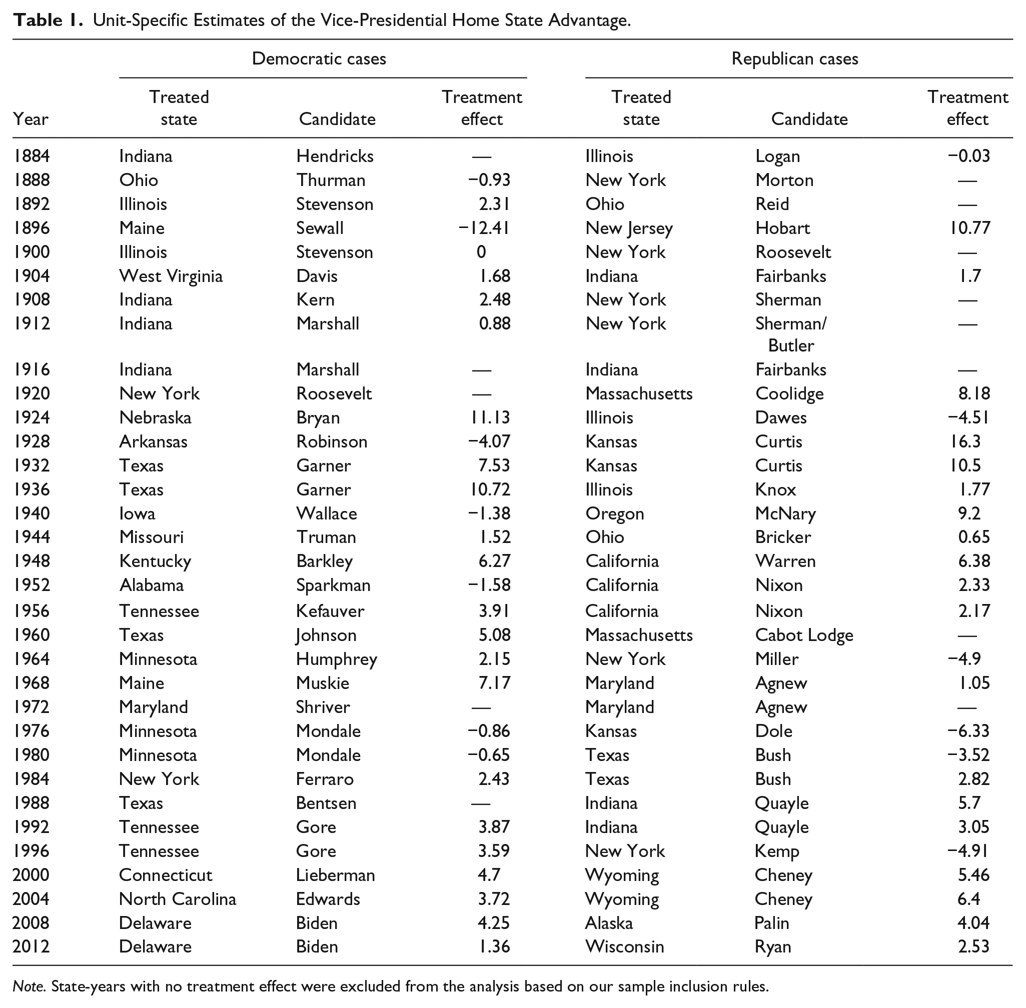
Note. State-years with no treatment effect were excluded from the analysis based on our sample inclusion rules.

Despite our earlier objections to the method for statistical inference proposed by Abadie et al. (2010), it has the significant advantage of being estimable for singular cases. Because any approach to inference at an aggregate level—including our own—assumes that treated and non-treated cases across different years are drawn from the same “treated distribution” and “non-treated distribution,” respectively, we use Abadie et al.’s (2010) method to provide estimates of “extremeness” for each individual case, relative to untreated cases in the same election year. Again, we note objections to this approach, particularly that unit-specific p values are underestimated, because treatment is not ignorable across units in the same election year. This objection motivated our decision to use randomization inference, but we report p values calculated using Abadie et al.’s (2010) method in the interest of estimating case-level uncertainty, despite its drawbacks.

We rank each treated case compared with all non-treated cases on the basis of effect size in the same election year and calculate the p value as the rank over the total number of cases in that year, applying Abadie et al.’s (2010) method to each treated case in our sample. Under the null hypothesis of no effect, the distribution of p values calculated in this way should be uniform on the unit interval. Figure 6 plots our 53 effect estimates and their p values and shows that the distribution is heavily skewed toward positive effect estimates and small p values—highly suggestive of a positive average effect.³⁴

Figure 6.

Distribution of Effect Estimates and p Values for Each Treated Case.

Falsification and Robustness Checks

Our investigation shows a positive and substantial effect of vice-presidential candidates on the two-party vote share in their home states. Our conclusions differ markedly from past findings. To increase confidence in our results and guard against specific threats to inference, we subject our findings to a series of falsification tests and robustness checks.

In our first falsification test, we exploit the fact that a state’s treatment in our study is time-limited. Vice-presidential candidates are on the ticket for one or two terms and then either exit the ticket or run as presidential candidates themselves. If a state is represented on the ticket in just one election, any increase we observe from the HSA should dissipate in the next election. Among our sample, there are 25 such cases, in which a state was represented on one of the major-party tickets in precisely one consecutive election. In Figure 7, we restrict the sample to these “singletons” and plot the gap in two-party vote share in times $t - 2$ through $t + 2$ between the 25 treated cases and their synthetic control units.³⁵ The effect size estimated in this sub-sample is dramatically smaller than our main result—unsurprising, given that these 25 vice-presidential candidates were almost uniformly on losing tickets. The key result is clear, however: Vote share in the home state, relative to the synthetic control unit, spikes during the treated election and then falls back to normal as soon as the state is no longer treated.³⁶

Figure 7.

The gap in vote share between treated and synthetic control units, among those treatment cases which lasted a single election cycle.

An additional threat to valid inference comes from interpolation biases. In practice, a synthetic control unit could be composed of highly dissimilar states that, when combined, mimic the pre-treatment outcomes in the treated unit. A simple example of such a phenomenon would be to combine highly Democratic Washington, D.C. and highly Republican Utah to create a synthetic control unit for Wisconsin in 2012. Abadie et al.’s (2010) suggestion in this regard is to trim the pool of donor units, limiting the pool to those states that would provide sensible matches to the treated unit. We trim on the basis of vote share in $t - 1,$ limiting the pool of possible donor units for each treated case to those states that most closely match the treated unit’s vote share in the prior election. Because there is little guidance on this topic in the literature, we experimented with three alternatives. We trimmed the pool of donor states to increasingly dramatic degrees, alternately dropping 10%, 25%, and 50% of the donor pool for each treated unit.³⁷ These approaches generate poorer quality matches on average, but do not have significant effects on our main findings: When we trim the donor pool by 10% and 50%, our effect estimates change from 2.67 to 2.78 and 2.20 percentage points, respectively. These results are shown in Figure 5, and additional details are provided in the supplemental appendix.

A further source of potential bias in our results arises from the regional appeal a running mate might have. For instance, those who argue LBJ was selected as a running mate who could deliver Texas often suggest this was part of a larger strategy by the Kennedy campaign to improve the ticket’s chances across the South, violating the no-spillover assumption needed for valid inference. However, to the extent that the states that make up our synthetic control units are often geographically proximate to the treated unit, this possibility would only serve to reduce the estimated advantage vice-presidential candidates provide in their home states. If, for example, Johnson improved the Democrats’ performance in Mississippi and Florida—the two states that comprise our synthetic control unit for Texas—then our results actually underestimate the vice-presidential HSA.

The results we have presented are both substantively meaningful and statistically significant according to our permutation tests. We have also shown that the treatment effect is temporally bound in cases in which treatment lasts for a single electoral period, and that our results are robust to—or even underestimated because of—the most likely sources of bias. As a final check on our results, in the next section, we investigate several cases in which our results diverge most dramatically from the findings of past studies.

Sensitivity Analysis of Divergent Cases

How do our individual estimates compare with those of previous studies? As would be expected, in several cases, there are sizable differences between our estimates and those of Devine and Kopko (2011). To further check the quality of our estimates, we subjected our results to two additional tests concerning “divergent cases”—those cases in which our estimates differ most dramatically from those of past studies. For eight divergent cases, we use a simple sensitivity analysis suggested by Abadie et al. (2015). For each case, we take the list of states that were included in the synthetic control, iteratively drop two at a time, and re-estimate the unit treatment effect.³⁸

Consider Massachusetts in 1920, whose synthetic control unit consists of New Hampshire, Rhode Island, Vermont, and North Carolina, in order of decreasing weight. In a first iteration, we remove New Hampshire and Rhode Island from the pool of possible donor states to the synthetic control and re-estimate; our effect estimate drops from 8.2 points to 5.6 points, and the synthetic control is constructed from Connecticut, Vermont, Texas, and Georgia, respectively. In a second iteration, we remove New Hampshire and Vermont from the analysis, and allow Rhode Island to return to the donor pool. We repeat this process, removing two states at a time from the pool, until we have exhausted all possible combinations.

In general, the primary synthetic control units that we report in our main results are prima facie logical. Arbitrary limitations on the states included in the donor pool, by design, never improve the pre-treatment fit between treated and control units.³⁹ However, our confidence in this formal approach to donor selection is buttressed by the fact that we generally prefer our primary synthetic control unit to the available alternatives on qualitative, case-specific grounds as well.

The results from our sensitivity analysis are summarized in Figure 8, which—for each of the eight cases—plots our primary estimate in a gray circle and each alternative estimate in hollow circles versus estimates generated by Devine and Kopko (2011) in gray squares. We find very few substantively important differences in estimates across available alternatives. In most cases, the alternatives return effect sizes similar to the primary results we report; more importantly, there does not appear to be any systematic bias in our primary estimates toward a larger-than-normal effect size.

Figure 8.

Primary models, alternative models, and a comparison with Devine and Kopko’s model for “divergent cases.”

Conclusion and Implications

In this article, we have attempted to solve a problem common to the study of strategic choices in electoral campaigns: estimating the counterfactual outcome in a world where the strategic choice was not made. Our assessment of the vice-presidential HSA shows the limitations of existing approaches in this regard. Our solution is to apply the synthetic control method for comparative case studies to an instance with multiple treated units. We argue that this approach allows us to estimate the vice-presidential HSA without biases that plagued earlier studies.

In academic literature, as well as in assessments of modern presidential campaigns by politicians and members of the media, it has become conventional wisdom that vice-presidential candidates are, electorally speaking, nearly irrelevant—generally unable even to affect the vote in their own home states. We argue that this viewpoint is partly based on an HSA measurement with considerable inherent flaws. In contrast, our results suggest that the average vice-presidential candidate improves his or her tickets’ performance in his or her home state by 2.67 points of the two-party vote.

The effect size we estimate is close to that attributed to presidential candidates, and can have substantial consequences for electoral outcomes within particular states. From our sample of 1,524 total state-year elections, a 2.67 percentage point improvement in vote share would have swung the outcome to the opposing party in 294 elections, or 19.3% of state-years. Although most presidential elections are not decided by a single state, a 2.67-point swing in a single state can still affect the outcome of the presidential election as a whole. For example, had a strategically optimal running mate been available and selected, and had she produced at least a 2.67-point effect, such a choice would have swung the 1960 and 1976 elections to the Republican side, and the 2000 and 2004 elections to the Democrats. Specifically, a 2.67-point bump in New York in either 1960 or 1976 would have resulted in a Republican electoral college win. An increase of 2.67 points in any of six states (Florida, Missouri, Nevada, New Hampshire, Ohio, or Tennessee) in 2000 or two states (Florida or Ohio) in 2004 would have resulted in Democratic victories.⁴⁰

Although there is broad consensus among political scientists that the “fundamentals” are mostly responsible for shaping the outcomes of presidential elections, strategic choices are still ubiquitous in election campaigns. These include the type of choices campaigns make on a day-to-day basis, from having candidates hold campaign appearances in specific locations to buying advertisements in specific media markets. Studying the effect these choices have on electoral outcomes presents a minefield of inferential problems. We believe our use of the synthetic control method to estimate the vice-presidential HSA can serve as a blueprint for investigating the impact of many other strategic choices in election campaigns. Strategic choices are unlikely to single handedly change the winner of most elections. However, strategic decisions aggregate over the life of a campaign. Indeed, even taken in isolation, we have shown that the choice of a vice-presidential running mate could have altered the outcome in several key elections over the last 60 years.

Footnotes

Declaration of Conflicting Interests

The author(s) declared no potential conflicts of interest with respect to the research, authorship, and/or publication of this article.

Funding

The author(s) received no financial support for the research, authorship, and/or publication of this article.

Notes

Author Biographies

Boris Heersink is a PhD candidate in Political Science at the University of Virginia. He studies American political party organizations, presidential campaigns and elections, and Southern politics.

Brenton D. Peterson is a PhD candidate in Political Science at the University of Virginia and a Research Affiliate at Strathmore University. He studies African politics, ethnicity and political methodology.

References

Abadie

Diamond

Hainmueller

(2010). Synthetic control methods for comparative case studies: Estimating the effect of California’s tobacco control program. Journal of the American Statistical Association, 105, 493-505.

Abadie

Diamond

Hainmueller

(2011). Synth: An R package for synthetic control methods in comparative case studies. Journal of Statistical Software, 42, 1-17.

Abadie

Diamond

Hainmueller

(2015). Comparative politics and the synthetic control method. American Journal of Political Science, 59, 495-510.

Abadie

Imbens

G. W.

(2008). On the failure of the bootstrap for matching estimators. Econometrica, 76, 1537-1557.

Acemoglu

Johnson

Kermani

Kwak

Mitton

(2013, December). The value of connections in turbulent times: Evidence from the United States (NBER Working Paper No. 19701). Retrieved from http://www.nber.org/papers/w19701

Black

(1973). The Wallace vote in Alabama: A multiple regression analysis. Journal of Politics, 35, 730-736.

Brogan

D. W.

(1954). Politics in America. New York, NY: Harper.

Carson

J. L.

Jenkins

J. A.

(2011). Examining the electoral connection across time. Annual Review of Political Science, 14, 25-46.

Carson

J. L.

Roberts

J. M.

(2007). Strategic politicians and U.S. House elections, 1874-1914. Journal of Politics, 67, 474-496.

10.

Congressional Quarterly Press. (2010). Guide to U.S. elections. Washington, DC: Author.

11.

Devine

C. J.

Kopko

K. C.

(2011). The vice presidential home state advantage reconsidered: Analyzing the interactive effect of home state population and political experience, 1884-2008. Presidential Studies Quarterly, 41, 1-17.

12.

Devine

C. J.

Kopko

K. C.

(2013). Presidential versus vice presidential home state advantage: A comparative analysis of electoral significance, causes and processes, 1884-2008. Presidential Studies Quarterly, 43, 814-838.

13.

Dudley

R. L.

Rapoport

R. B.

(1989). Vice-presidential candidates and the home state advantage: Playing second banana at home and on the road. American Journal of Political Science, 33, 537-540.

14.

Erikson

R. S.

Wlezien

(2012). The timeline of presidential elections. Chicago, IL: University of Chicago Press.

15.

Fisher

R. A.

(1935). The design of experiments. London, England: Oliver and Boyd.

16.

Fowler

(2013). Electoral and policy consequences of voter turnout: Evidence from compulsory voting in Australia. Quarterly Journal of Political Science, 8, 159-182.

17.

Garand

J. C.

(1988). Localism and regionalism in presidential elections: Is there a home state or regional advantage? The Western Political Quarterly, 41, 85-103.

18.

Grofman

Kline

(2010). Evaluating the impact of vice presidential selection on voter choice. Presidential Studies Quarterly, 40, 303-309.

19.

D. E.

Imai

King

Stuart

E. A.

(2007). Matching as nonparametric preprocessing for reducing model dependence in parametric causal inference. Political Analysis, 15, 199-236.

20.

Holbrook

T. M.

(1991). Presidential elections in space and time. American Journal of Political Science, 35, 91-109.

21.

Jacobson

G. C.

Kernell

(1981). Strategy and choice in congressional elections. New Haven, CT: Yale University Press.

22.

Keele

McConnaughy

White

(2012). Strengthening the experimenter’s toolbox: Statistical estimation of internal validity. American Journal of Political Science, 56, 484-499.

23.

Key

V. O.

(1949). Southern politics in state and nation (1st ed.). Knoxville: University of Tennessee Press.

24.

Kolodny

(1998). Pursuing majorities: Congressional campaign committees in American politics. Norman: University of Oklahoma Press.

25.

Kreif

Grieve

Hangartner

Turner

A. J.

Nikolova

Sutton

(2015). Examination of the synthetic control method for evaluating health policies with multiple treated units. Health Economics. Advance online publication. doi:10.1002/hec.3258

26.

Ladd

J. M.

Lenz

G. S.

(2009). Exploiting a rare communication shift to document the persuasive power of the news media. American Journal of Political Science, 53, 394-410.

27.

Lewis-Beck

M. S.

(2005). Election forecasting: Principles and practice. British Journal of Politics and International Relations, 7, 145-164.

28.

Lewis-Beck

M. S.

Rice

T. W.

(1983). Localism in presidential elections: The home state advantage. American Journal of Political Science, 27, 548-556.

29.

Liou

Y. M.

Musgrave

(2014). Refining the oil curse: Country-level evidence from exogenous variations in resource income. Comparative Political Studies, 47, 1584-1610.

30.

Romero

D. W.

(2001). Requiem for a lightweight: Vice presidential candidate evaluations and the presidential vote. Presidential Studies Quarterly, 31, 454-463.

31.

Rosenbaum

P. R.

(2002). Covariance adjustment in randomized experiments and observational studies. Statistical Science, 17, 286-327.

32.

Rosenstone

S. J.

(1983). Forecasting presidential elections. New Haven, CT: Yale University Press.

33.

Rove

(2012, April 25). I was wrong about Dick Cheney. The Wall Street Journal, Op-ed.

34.

Shaw

D. R.

(2006). Race to 270: The electoral college and the campaign strategies of 2000 and 2004. Chicago, IL: University of Chicago Press.

35.

Sides

Vavreck

(2013). The gamble: Choice and chance in the 2012 presidential election. Princeton, NJ: Princeton University Press.

36.

Sigelman

Wahlbeck

P. J.

(1997). The “veepstakes”: Strategic choice in presidential running mate selection. American Political Science Review, 91, 855-864.

37.

Silbey

J. H.

(2010). Regimes, epochs, state authority, and the nature of American political life over two centuries. Historical Methods, 43, 171-174.

38.

Tatalovich

(1975). “Friends and neighbors” voting: Mississippi, 1943-73. Journal of Politics, 37, 807-814.

39.

Wawro

G. J.

Katznelson

(2014). Designing historical social scientific inquiry: How parameter heterogeneity can bridge the methodological divide between quantitative and qualitative approaches. American Journal of Political Science, 58, 526-546.

40.

Woolley

J. T.

Peters

(2013). The American presidency project (Online Repository). Available from http://www.presidency.ucsb.edu/

41.

(2015). Generalized synthetic control method for causal inference with time-series cross-sectional data (MIT Political Science Department Research Paper No. 2015-1). Retrieved from http://ssrn.com/abstract=2584200