Accelerated Brain DCE-MRI Using Iterative Reconstruction With Total Generalized Variation Penalty for Quantitative Pharmacokinetic Analysis: A Feasibility Study

Abstract

Purpose:

To investigate the feasibility of using undersampled k-space data and an iterative image reconstruction method with total generalized variation penalty in the quantitative pharmacokinetic analysis for clinical brain dynamic contrast-enhanced magnetic resonance imaging.

Methods:

Eight brain dynamic contrast-enhanced magnetic resonance imaging scans were retrospectively studied. Two k-space sparse sampling strategies were designed to achieve a simulated image acquisition acceleration factor of 4. They are (1) a golden ratio–optimized 32-ray radial sampling profile and (2) a Cartesian-based random sampling profile with spatiotemporal-regularized sampling density constraints. The undersampled data were reconstructed to yield images using the investigated reconstruction technique. In quantitative pharmacokinetic analysis on a voxel-by-voxel basis, the rate constant K ^trans in the extended Tofts model and blood flow F _B and blood volume V _B from the 2-compartment exchange model were analyzed. Finally, the quantitative pharmacokinetic parameters calculated from the undersampled data were compared with the corresponding calculated values from the fully sampled data. To quantify each parameter’s accuracy calculated using the undersampled data, error in volume mean, total relative error, and cross-correlation were calculated.

Results:

The pharmacokinetic parameter maps generated from the undersampled data appeared comparable to the ones generated from the original full sampling data. Within the region of interest, most derived error in volume mean values in the region of interest was about 5% or lower, and the average error in volume mean of all parameter maps generated through either sampling strategy was about 3.54%. The average total relative error value of all parameter maps in region of interest was about 0.115, and the average cross-correlation of all parameter maps in region of interest was about 0.962. All investigated pharmacokinetic parameters had no significant differences between the result from original data and the reduced sampling data.

Conclusion:

With sparsely sampled k-space data in simulation of accelerated acquisition by a factor of 4, the investigated dynamic contrast-enhanced magnetic resonance imaging pharmacokinetic parameters can accurately estimate the total generalized variation-based iterative image reconstruction method for reliable clinical application.

Keywords

brain DCE-MRI pharmacokinetic analysis total generalized variation iterative reconstruction

Introduction

Dynamic contrast-enhanced magnetic resonance imaging (DCE-MRI) is an advanced MR technique that can be used as a noninvasive imaging tool for the measurement of microvascular properties. Based on the rapid acquisition of a series of images before, during, and after the intravenous administration of a low-molecular-weight contrast agent (CA), DCE-MRI is sensitive to differences in blood flow, blood volume, and vascular permeability that can be associated with tumor angiogenesis.¹ By fitting the DCE-MRI data to certain pharmacokinetic (PK) models, volumetric maps of quantitative physiological parameters can be obtained in PK model analysis. Compared with computed tomography in probing microvascular characteristics, DCE-MRI has a higher sensitivity to CA with no use of ionizing radiation.² In addition, as a functional imaging method against the functional nuclear medicine imaging methodology including positron emission tomography and single-photon emission computed tomography, DCE-MRI has the distinguishing feature of combining morphological and functional information acquirement in a single imaging session with potentially improved spatial resolution.³ Because of these merits, DCE-MRI is a promising method for various clinical oncologic tasks and has been investigated in early diagnosis,^4,5 tumor staging,⁶ treatment planning,^7,8 and treatment response assessment.^9

–13

Of all possible factors that may influence the accuracy in either semiquantitative or quantitative DCE-MRI analysis, temporal resolution (Δt) is well documented as an important one.^14,15 Because of the dynamic nature of DCE-MRI, high temporal resolution is desirable. In particular, the arterial input function (AIF), which depicts the CA dynamics within the feeding arterial blood, has to be determined via imaging a major arterial structure that exists in the imaging volume with high temporal resolution.^16,17 To ensure the accuracy of PK analysis, the reliable AIF information derivation demands 1 second or faster temporal resolution in image acquisition to accurately capture the rapid washin and washout processes of CA in arterial blood.^18,19 However, owing to the limited volume acquisition time or lack of arterial structure within the image volume, the individualized AIF measurement may not always be feasible.²⁰ By assuming the similar CA dynamics of different subjects, population-derived mathematical AIF models have been proposed.^21
–23 However, these simplified models ignore the potentially large physiological variability among subjects and may introduce additional errors to the PK analysis.²⁴ Additionally, insufficient temporal resolution may also affect the accuracy of PK analysis by introducing intensity uncertainties in the CA concentration measurement of tissue of interest. It has been noted by both imaging and simulation studies that when accurate AIF information was available, the error of CA rate constants increases as the temporal resolution degrades.^25,26 As a result, improving temporal resolution is of particular interest in DCE-MRI studies toward the clinical application.¹²

To accelerate DCE-MRI acquisition, various fast imaging methods using reduced k-space data sampling, such as sliding window (SW), 3D keyhole,^27,28 and k-t Broad-use linear acquisition speed-up technique,²⁹ have been proposed and investigated. In recent years, the theory of compress sensing (CS) proved that at the violation of classic Nyquist theorem, a small sampling fraction in certain patterns is sufficient to reconstruct compressible signals using a linear reconstruction subject to a specified penalty.^30
–32 The sparsity implicit in MR images under Fourier transformation suggests the great potential of CS in the acceleration of MRI studies. To date, CS application in dynamic MR has been successfully demonstrated in many studies.^33

–36 As for DCE-MRI, several studies have been conducted in the past to investigate CA rate constants using the reconstructed images with undersampled patient and animal data.^37

–41 In these studies, the concept of total variation (TV) based on the first-order derivative calculation was commonly adopted in the constrained image reconstruction to minimize the gradient of the reconstructed image.⁴² In spite of its popularity, the concept of TV relies on the assumption that MR image consists of piecewise constant regions, yet this assumption may not always be valid in human MR imaging with the potential inhomogeneity of exciting field.⁴³ With the existence of staircasing artifacts, the accuracy of TV-based reconstructed image may be compromised. The staircasing artifacts may further affect the accuracy of PK parameter map calculation in DCE-MRI. Another problem in these studies is that the AIF was approximated by published models or previously reported measurements, and these approximations may lead to errors in the evaluation of undersampling effect. Furthermore, few studies have been conducted to explore the feasibility of using undersampled k-space data for quantitative blood perfusion analysis.

In this study, we explored the clinical feasibility of using undersampled k-space data for quantitative analysis with 2 commonly adopted DCE-MRI PK models. Clinical brain DCE-MRI scans were used, and 2 k-space data sampling strategies were proposed to achieve an acceleration factor of 4. In the iterative image reconstruction, a penalty term based on the recently developed mathematical concept of second-order total generalized variation (TGV) was adopted.⁴⁴ In the PK analysis, individualized AIF information was measured, and the accuracy of our approach was investigated via the quantitative evaluation of the derived PK parametric maps.

Materials and Methods

Reference Data

Eight sets of brain DCE-MRI scans from 6 patients with recurrent malignant glioma were selected from an institutional review board-approved clinical study as the reference images. The scans were acquired in the axial plane using a bird-cage quadrature head coil and a 3-dimensional (3D) spoiled-gradient recalled echo sequence on a clinical 1.5T scanner (General Electric, Fairfield, Connecticut). Each set of scan consists of preinjection calibration volumes at various flip angles and 60 postinjection volumes, and the temporal resolution was about 5.25 seconds of each volume (image matrix size: 256 × 256; acquisition matrix size: 256 × 128). The k-space data of the clinical scans were saved as the full sampling data in this study, and the undersampled k-space data were generated via sampling the full data with 2 specific undersampling strategies discussed subsequently.

Radial-Based Sampling Scheme

Because of a good balance of central/peripheral sampling weights with good low-frequency coverage and potentially improved point spread function,⁴⁵ an optimized radial-based undersampling profile with multiple spokes was investigated to demonstrate the mathematical accuracy of this TGV-based reconstruction algorithm. Specifically, in this work, the undersampled k-space data were generated by sampling each slice of the full sampling data with a 32 non-Cartesian-ray radial sampling profile defined on a Cartesian grid.³⁹ Related to the golden ratio, the sampling profile was generated by a constant azimuthal increment of Δβ = 111.25° (Figure 1),⁴⁶ and radial rays were evenly spaced with time.⁴⁷ This sampling pattern acquired approximately 11.5% of full k-space area and simulated an accelerated image acquisition by a factor of 4. Compared to the even-distributed sampling profile, the sampling efficiency of this golden ratio–based profile has no difference.⁴⁸ Radial rays were evenly spaced with time, and only 3 different azimuthal gaps occurred in comparison with the evenly distributed rays. Thus, this sampling profile allows a posteriori adjustment of the temporal resolution.⁴⁹

Figure 1.

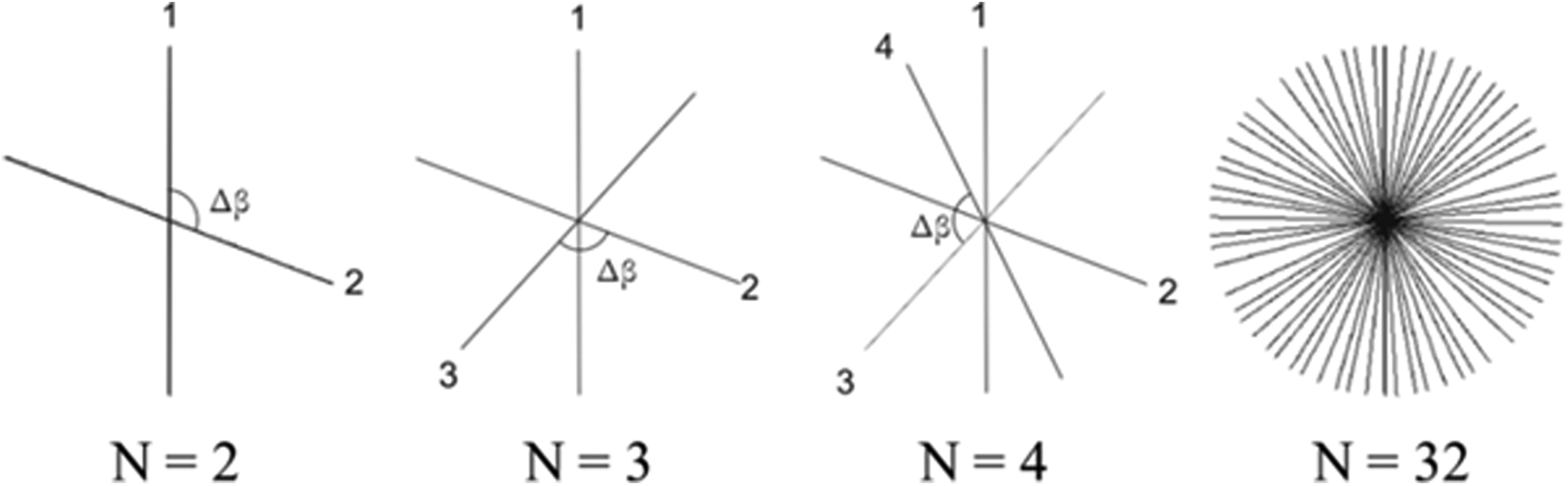
Generation of the 32-ray radial sampling pattern at a golden ratio angular increment.

Cartesian-Based Sampling Scheme

Although radial sampling profile has its advantages for limited k-space acquisition, the higher demand for hardware implementation inhabits its application on most clinical task-oriented scanners. Besides, image reconstruction from radially sampled data requires certain regridding approaches that are often far from trivial.⁵⁰ In contrast, sampling profiles defined in Cartesian coordinate system are straightforward and are suitable for easy implementation. However, because of evenly distributed sampling density on the frequency-encoding direction, more readout lines are required to achieve an adequate k-space coverage for backprojection. Early efforts were made to integrate SW technique into Cartesian undersampling profile sequences.⁵¹ Although the feasibility was demonstrated, the achieved acceleration factor was limited without proper indication of possible application in DCE-MRI.

Based on above issues, a novel Cartesian-based sampling profile sequence with integrated SW technique was designed as the second sampling scheme of this work. First, a variable Poisson ellipsoid spatial sampling density function was built as demonstrated in Figure 2.

Figure 2.

Illustration of a 2-dimensional (2D) sampling profile with variable sampling density. The central red region is fully sampled, and the rest in gray level is sampled with varying sampling density.

Specifically, for each 2-dimensional (2D) full profile covered in the original acquisition of the clinical scan, the central 15% of k-space along the phase-encoding direction was fully sampled (indicated by red color). Then, the rest k-space region was treated as high-frequency (HF) sampling region, and each side of the region was evenly divided into 4 subregions along the phase-encoding direction. Each subregion was assigned a uniform sampling density ρ _i , which decreases exponentially from k-space center (indicated by gray levels with color bar):

ρ_{i} = ρ_{0} e^{- r_{i} / τ}

where ρ₀ is the scaling factor to ensure the probability density normalization. The parameter r_i indicates the relative length (in phase-encoding direction) if the ith HF subregion in reference to the total HF region length, and the dimensionless decay constant τ was chosen as 1. In this work, HF data in 10% of the original k-space size was acquired in the designated HF region. Thus, an acceleration of 4 was achieved by sampling each 2D reference data with 25% data size (15% in central region and 10% in HF region).

For a series of 2D k-space data at a certain location in the dynamic scan, the SW technique was applied by inserting HF data acquired in 2 adjacent frames into the HF region of the k-space to be constructed. Figure 3 shows the schematic of SW in the HF region. In the first row, at each time point, k-space data were acquired using the variable density profile in Figure 2. For the k-space to be reconstructed at time point t₁ in the second row, the HF region was filled by HF data from t₀ , t₁ , and t₂ points, while central k-space region was filled with data only from t₁ central k-space data. To achieve a higher k-space coverage ratio, temporal constraints were added to Equation 1 to ensure that sampled HF regions have no overlap within each k-space triplet. The synthesized k-space slices were then used for image reconstruction.

Figure 3.

A schematic of sliding window (SW) with variable density Cartesian sampling profiles. Each black line represents a sampled readout line.

Image Reconstruction

Using each data sampling scheme, the undersampled data were then used for Cartesian MR reconstruction in an inverse problem with a penalty term of TGV theory:

{argmin}_{u} {| | F (u) - k | |}_{2}^{2} + {β TGV}^{2} (u),

where u represents the reconstructed image, F represents Fourier transform, k represents the undersampled k-space data, and β denotes the regularization parameter for the TGV penalty term. The TGV penalty term can be organized as⁴⁴:

{TGV}^{2} (u) = {min}_{v} {\int_{Ω} | \nabla u - v | dx + α \int_{Ω} \frac{1}{2} | \nabla v + \nabla v^{T} | dx},

where the minimum is taken over all vector fields on Ω, and v is an introduced test function in the same order as the first-order derivative of the reconstructed image (∇u). At the neighborhood of edges on the image, the test function v approximates the first-order derivative of the image, and the first integration term in Equation 3 preserves the edge information as the optimal outcome. On the other hand, the symmetric derivative of v in the second integration term of Equation 3 improves the smoothness of the image based on the observation that second-order derivative (∇²u) is locally small within the smooth region of the image. The parameter α is used to keep a balance between the first- and second-order derivatives of the image. Thus, the TGV penalty term regularizes the features on both smooth and sharp region of the image. The nonlinear inversion in Equation 2 can be approximated using the iterative-regularized Gaussian-Newton method.^52
–54 At each step n for the given uⁿ , update the δu of the minimization problem:

{min}_{δ} {| | F^{'} (u^{n}) δ u + F (u^{n}) - k | |}^{2} + 2 β_{k} {TGV}^{2} (u^{n} + δ u),

which can be estimated efficiently using the first-order primal dual algorithm.^55
–57 As in the reconstruction, no reference image was used. In Equation 2, α was set to 2 based on our experience for best brain imaging accuracy⁴³; the initial value of β _k was set as 1, and its attenuation factor along iterations was empirically chosen as 5. The maximum iteration step was set to 8 in the consideration of a balance between image accuracy and computation cost.

Pharmacokinetics Analysis

Pharmacokinetics analysis with same procedures was conducted using the reference clinical image series as well as the image series reconstructed from undersampled k-space data with 2 difference sampling schemes, respectively. In order to quantify the CA concentration C(t), a linear relationship between the 2 quantities is assumed:

\frac{1}{T_{1} (t)} = r_{1} C (t) + \frac{1}{T_{10}},

where T ₁₀ is the preinjection T ₁ value, T ₁(t) is the changed T ₁ value at each time point after the injection, and r ₁ is the longitudinal relaxivity of CA at 1.5T magnetic field strength. Both T ₁₀ and T ₁(t) were calculated voxel-by-voxel using the standard dual flip angle method,⁵⁸ and flip angles 5° and 15° were used. The CA concentration distribution at each time point was then calculated by Equation 5 and was processed by a denoising method.⁵⁹ The CA concentration–time curve in the arterial blood C _p(t) (AIF) was measured in the way as described below: first, an arterial structure within the intracranial imaging volume was carefully contoured in 3D fashion by a clinical professional. Then a histogram of each arterial structure voxel’s time-to-peak (T _max) was generated.⁶⁰ Next, the T _max of the C _p(t) was determined by the peak position of the generated histogram, and the C _p(t) was calculated by averaging the CA concentration of the voxels that constituted the histogram’s peak.

Two commonly used PK models were investigated in this study. First, the extended Tofts model was analyzed to quantify K ^trans, which has served as the primary quantitative imaging biomarker in many oncologic DCE-MRI studies.^14,61 This model assumes that CA exchanges between the blood plasma and extravascular extracellular space (EES) and the CA concentration in tissue of interest C _t (t) can be expressed as⁶²:

C_{t} (t) = K^{trans} \int_{0}^{t} C_{p} (u) \cdot e^{- k_{ep} (t - u)} du + v_{p} \cdot C_{p} (t),

where K ^trans describes CA extravasation rate from blood vessel to EES, k_ep = K^trans/v_e represents the rate constant of CA from EES back to blood plasma, and v _e and v _p denote the volume fractions of EES and blood plasma, respectively. The parameters were determined by a linear least squares-based curve fitting method.⁶³

The 2-compartment exchange model was used to quantify the blood flow and blood volume.^64,65 Following the conservation of CA mass, C _t (t) is expressed as:

C_{t} (t) = F_{B} \int_{0}^{t} C_{p} (u) \cdot [e^{- K_{+} (t - u)} + E (e^{- K_{-} (t - u)} - e^{- K_{+} (t - u)})] du,

where F _B stands for blood flow, K _± were related to the reciprocal CA exchange rate constants between blood plasma and tissue of interest, and E is a parameter associated with K _± and circulation transit time T_T. Fitting Equation 7 with C_p(t) and C _t (t) by Levenberg-Marquardt algorithm with zero initial conditions,⁶⁶ T_T can be calculated as:

T_{T}^{- 1} = K_{+} - E (K_{+} - K_{-}),

and blood volume V _B can be estimated as:

V_{B} = F_{B} \cdot T_{T} .

Quantitative Accuracy Analysis

The investigated PK parameters (K ^trans, F _B, and V _B) were calculated in a voxel-by-voxel pattern, and 2 sets of parameter maps were generated from the original clinical scan image (full sampling set) and the reconstructed images using undersampled data (reduced sampling set), respectively. For the purpose of quantitative accuracy evaluation, a 3D region of interest (ROI) was defined using gross tumor volume from the radiotherapy treatment planning system. As the most commonly reported metrics in clinical studies, the means of K ^trans, F _B, and V _B across the ROI were compared for relative differences. For each parameter, we used the “error in volume mean (EIVM)” for the PK parameters estimation accuracy⁴⁰:

EIVM (P) = \frac{\overline{P_{r} (x, y, z)} - \overline{P_{f} (x, y, z)}}{\overline{P_{f} (x, y, z)}} \times 100 %,

where the P _r(x,y,z) and P _f(x,y,z) denote the parameter’s distributions within the ROI from the reduced sampling set and the full sampling set, respectively, and the overhead bar represents the average across ROI. For voxel-based analysis, a histogram depicting the parameter’s calculation difference using reduced sampled data was generated. The parameter’s difference map within the ROI was also evaluated. The accuracy was further evaluated using the 2 quantitative metrics: total relative error (TRE) and cross-correlation (CC). The TRE is defined as follows⁶⁷:

TRE = \frac{\sqrt{\sum_{x, y} {[P_{r} (x, y, z) - P_{f} (x, y, z)]}^{2}}}{\sqrt{\sum_{x, y} {[P_{f} (x, y, z)]}^{2}}},

where P _r(x,y,z) and P _f(x,y,z) follow the same definitions in Equation 10. The CC was calculated to measure the similarity of a certain parameter’s distributions from the 2 parameter maps sets:

CC = \frac{\sum_{i} (P_{r, i} - \bar{P_{r}}) (P_{f, i} - \bar{P_{f}})}{{(\sum_{i} {(P_{r, i} - \bar{P_{r}})}^{2})}^{1 / 2} {(\sum_{i} {(P_{f, i} - \bar{P_{f}})}^{2})}^{1 / 2}},

where the summation was calculated within the 3D ROI, and the overhead bar represents the mean value. To determine the significance levels of the differences between the PK parameter results using full sampling data and reduced sampling data, Wilcoxon signed rank test was adopted. Statistical significance was defined as α < .05 with multiple comparison correction.

All image reconstruction works and PK analysis were carried out in a software developed in-house using MATLAB (R2012b; MathWorks Inc, Natick, Massachusetts) on a personal desktop with 16 GB RAM and 3.4 GHz central processing unit. As for efficiency evaluation, computation time was measured using functions “tic” and “toc” in MATLAB.

Results

Radial-Based Sampling Scheme Results

Figure 4 shows a selected patient’s 2D comparison of the original clinical DCE image (A) and the reconstructed image using the undersampled data from the radial-based sampling scheme (B). The images were from a postinjection volume, and the red contour line indicates the ROI for quantitative analysis. As can be seen, (B) preserved most structural details in (A), though some details were lost at high-intensity region. The average TRE value of all patients’ reconstructed images using the radial-based sampling scheme was about 0.113. Figure 5 presents the comparison of measured AIF information, and C _p,f(t) and C _p,r(t) denote the AIF measured on the CA concentration maps derived from original clinical image set (blue) and the reconstructed image set (red), respectively. As can be seen, the peak positions of the 2 curves were identical, and the peak enhancements of C _p,f(t) and C _p,r(t) were 0.350 and 0.366 mmol/L, respectively. The shape features of C _p,f(t) were generally preserved by C _p,r(t), though C _p,r(t) had an overestimated intensity both before and after the first pass peak.

Figure 4.

A comparison of the original postinjection image (A) and the reconstructed image using the radial-based undersampled data (B). The intensity difference between (A) and (B) is shown in (C). The red contour indicates the region of interest (ROI) that contains the tumor.

Figure 5.

The comparison of the measured C _p(t) from the contrast agent (CA) concentration maps calculated from original clinical images (blue curve) and the images reconstructed from radial-based undersampled data (red curve).

Figures 6 to 8 demonstrate the comparison of PK parameter maps (K ^trans, F _B, and V _B) that correspond to the same imaging position shown in Figure 4. In each figure, the parametric maps calculated using the full sampling data and the reduced sampling data are presented in (A) and (B), respectively. The histogram (C) presents the distribution of the relative error of the 3D ROI parameter map in (B) versus (A). The PK parameters’ percentage difference map within the ROI is shown in (D). The results of K ^trans are presented in Figure 6. As can be observed, the 2 K ^trans maps were morphologically similar, and a K ^trans intensity-elevated region within the ROI (indicated by white arrows) was clearly identified on both maps. The heterogeneity of K ^trans intensity within the identified region in Figure 6A was successfully reproduced in Figure 6B. The histogram in (C) suggested an overall acceptable 3D K ^trans estimation accuracy using the reduced sampling data. The median value of absolute percentage difference in (C) was about 6.70%. The difference map in Figure 6D also suggested a good voxel-based quantitative calculation accuracy of K ^trans at the center of ROI, though minor discrepancies of K ^trans underestimation in Figure 6B were found at ROI peripheral region.

Figure 6.

A comparison of K ^trans map calculated using the original full sampling data (A) and using the radial-based undersampled data (B). The histogram about relative error of (B) versus (A) of all 3-dimensional (3D) region of interest (ROI) voxels (C). The histogram about relative error of (B) versus (A) of all 3D region of interest (ROI) voxels. (D). The percentage difference map of the 2D ROI between (A) and (B)

Figure 7.

A comparison of F _B map calculated using the original full sampling data (A) and using the radial-based undersampled data (B). The histogram about relative error of (B) versus (A) of all 3-dimensional (3D) region of interest (ROI) voxels (C). The histogram about relative error of (B) versus (A) of all 3D region of interest (ROI) voxels. (D). The percentage difference map of the 2D ROI between (A) and (B).

Figure 8.

A comparison of V _B map calculated using the original full sampling data (A) and using the radial-based undersampled data (B). The histogram about relative error of (B) versus (A) of all 3-dimensional (3D) region of interest (ROI) voxels (C). The histogram about relative error of (B) versus (A) of all 3D region of interest (ROI) voxels. (D). The percentage difference map of the 2D ROI between (A) and (B).

Figure 7 demonstrates the blood flow F _B results. On both Figure 7A and B, a circular region with elevated F _B was identified approximately at the K ^trans hot region shown in Figure 6A and B. Compared to the F _B-elevated region in Figure 7A, the identified region in Figure 7B had a minor difference at its right posterior boundary. The difference map in Figure 7D shows a good accuracy of F _B estimation in Figure 7B, and the left anterior region indicated a minor F _B underestimation in Figure 5A. The results of blood volume V _B are illustrated in Figure 8. As is the pattern indicated by K ^trans and F _B results, a region with elevated V _B values was indicated in Figure 8A and B. The V _B difference map in Figure 8D also exhibited the good V _B calculation accuracy using the reduced sampling data set.

As for the quantitative accuracy evaluation within the ROI in 3D fashion, Table 1 summarizes each PK parameter’s EIVM, TRE, and CC within the defined ROI of all 8 scans using the radial-based undersampling profile. The EIVM values demonstrated in Table 1 were all around 5% or less except one V _B EIVM value that indicated an 8.7% error. These results suggest that just as the commonly reported metrics in clinical studies, the mean values of the investigated PK parameters can be accurately calculated using the undersampled data. The TRE values varied from 0.08 to 0.15 with an average value of 0.11. As a description of the morphological similarity of 2 images, most CC values were higher than 0.95, and the observed smallest CC was 0.83. In the Wilcoxon signed rank tests, the statistical significance level of differences in K ^trans, F _B, and V _B were 0.528, 0.889, and 0.123, respectively. These results suggested that there is no significant differences between the PK maps calculated from the full sampling set and the one calculated from the reduced sampling set.

Table 1.

The Results of Error in Volume Mean (EIVM), Total Relative Error (TRE), and Cross-Correlation (CC) Within the 3D ROI Using Radial-Based Undersampled Data.

Patient No.	K ^trans			F _B		V _B
Patient No.	EIVM	TRE	CC	EIVM	TRE	CC	EIVM	TRE	CC
1	−0.65%	0.108	0.951	0.78%	0.086	0.981	−0.76%	0.100	0.987
2	5.17%	0.110	0.977	−1.29%	0.098	0.971	−4.33%	0.108	0.941
3^a	−1.53%	0.104	0.990	−3.00%	0.109	0.950	−0.12%	0.096	0.989
3^b	0.85%	0.129	0.979	−0.59%	0.128	0.955	6.49%	0.101	0.978
4	2.66%	0.102	0.960	1.54%	0.075	0.966	6.72%	0.121	0.996
4^b	−1.76%	0.129	0.926	−0.28%	0.131	0.967	−2.09%	0.134	0.981
5	5.90%	0.103	0.941	0.66%	0.097	0.827	−2.23%	0.105	0.943
6	<0.01%	0.133	0.944	−1.66%	0.086	0.944	−8.73%	0.146	0.943

Abbreviations: F _B, blood flow; V _B, blood volume; ROI, region of interest.

^aImages are selected from this scan.

^bSecond scan of this patient.

Cartesian-Based Sampling Scheme Results

Figure 9 shows the comparison of reference DCE image (A) and the reconstructed image using undersampled data from the Cartesian-based undersampling scheme (B) in the same organization as Figure 4. The DCE image in (B) preserves most structural details in (A), and the difference map in (C) indicates the discrepancies at boundaries. The average TRE values of all reconstructed images using the Cartesian-based undersampling scheme was about 0.109, and this number was very close to the corresponding number (0.113) when using the aforementioned radial-based sampling scheme. Figure 10 presents the comparison of measured AIF information from original clinical image (blue) and the reconstructed image (red), respectively. Similar to the results in Figure 5, the red curve has same peak position and fluctuation patterns as of the blue curve. The peak enhancement of the red curve was 0.382 mmol/L, which is more deviant from the 0.350 mmol/L value of the blue curve than the red curve in Figure 5 (0.366 mmol/L) with radial-based sampling scheme.

Figure 9.

A comparison of the original postinjection image (A) and the reconstructed image using the Cartesian-based undersampled data (B). The intensity difference between (A) and (B) is shown in (C). The red contour indicates the location of gross tumor volume (GTV) as region of interest (ROI).

Figure 10.

The comparison of the measured C _P(t) from the contrast agent (CA) concentration maps calculated from original clinical images (blue curve) and the images reconstructed from Cartesian-based undersampled data (red curve).

Figures S1, S2, and S3 in the supplementary material document summarize the K ^trans, F _B, and V _B results in the same organization as in Figures 6 to 8. For a short conclusion, all the 3 PK parametric maps that were reconstructed using the Cartesian-based undersampled data were very similar to the reference maps. For quantitative evaluations, each PK parameter’s EIVM, TRE, and CC of all the 8 scans are summarized as Table 2. The EIVM results in Table 2 were generally around 5% or less, but in some cases, the results were worse than the corresponding values in Table 1. The largest EIVM value in Table 2 is 16.67%. All observed CC values in Table 2 were higher than 0.9, and this result indicates the good morphological match of PK parametric maps using undersampled data. The average TRE values of all calculated PK parametric maps was about 0.122, and this number is higher than the corresponding result (0.111) using the radial sampling scheme. Additionally, no statistically significant results were found between the mean K ^trans (P = .950), F _B (P = .401), and V _B (P = .888) using reference data and using the undersampled data with Cartesian-based scheme.

Table 2.

The Results of Error in Volume Mean (EIVM), Total Relative Error (TRE), and Cross-Correlation (CC) Within the 3D ROI Using Cartesian-Based Undersampled Data.

Patient No.	K ^trans				F _B		V _B
Patient No.	EIVM	TRE	CC	EIVM	TRE	CC	EIVM	TRE	CC
1	6.92%	0.135	0.982	5.11%	0.119	0.961	4.40%	0.106	0.993
2	1.40%	0.135	0.967	6.81%	0.103	0.949	1.98%	0.135	0.994
3^a	2.01%	0.082	0.994	5.02%	0.110	0.977	0.80%	0.084	0.993
3^b	4.55%	0.147	0.935	−3.98%	0.110	0.968	−6.49%	0.121	0.972
4	−1.45%	0.137	0.980	1.40%	0.081	0.923	−5.94%	0.092	0.995
4^b	−4.41%	0.139	0.938	6.22%	0.111	0.994	−1.27%	0.152	0.983
5	−7.89%	0.108	0.990	−6.26%	0.162	0.763	−2.35%	0.149	0.965
6	2.81%	0.111	0.988	−3.96%	0.096	0.990	16.67%	0.155	0.995

Abbreviations: 3D, 3-dimensional; F _B, blood flow; V _B, blood volume; ROI, region of interest.

^aImages are selected from this scan.

^bSecond scan of this patient.

Discussion

In this pilot study toward potential clinical application, we investigated the feasibility of using undersampled k-space data for quantitative PK analysis in clinical brain DCE-MRI study. Particularly, we adopted a TGV penalty term in the iterative image reconstruction, and we analyzed the accuracy of PK parameters from 2 commonly used models using the undersampled data. Our results demonstrate that the investigated PK parameters can be accurately estimated using 2 data undersampling strategies at an acceleration factor of 4. In this part of the article, we further discuss several technical issues regarding the proposed methods in this work.

To ensure the accurate DCE image reconstruction, central k-space region needs to be sampled properly. Because of the superior central k-space sampling scheme, the radial sampling profile could use fewer rays than the Cartesian sampling profile to reach an acceptable central/peripheral k-space coverage balance. The golden ratio–optimized sampling profile is noteworthy. Mathematical deduction proved that when N = 32 rays were used, only 3 different azimuthal gaps occurred in comparison with the evenly distributed rays.⁴⁶ Thus, this sampling profile allows a posteriori adjustment of the temporal resolution.⁴⁹ In terms of sampling efficiency, this golden ratio–based profile has no difference with the uniform profile.⁴⁸ On the other hand, to achieve a same acceleration factor using Cartesian grid sampling, SW technique becomes important to guarantee the adequate k-space coverage. The comparison of the numerical TRE and EIVM results in Tables 1 and 2 suggest that the accuracy of PK parameters using Cartesian-based undersampled data was generally and yet slightly worse than using the radial-based undersampled data. In this work, the radial sampling profile was simulated at the Cartesian grid. Using this approach, the potential error from data gridding/regridding was not included, and the difference in reconstructed images to the reference came from the image reconstruction process only. As a feasibility investigation of the TGV algorithm, this is a good demonstration of the algorithm’s mathematical accuracy. For potential real clinical application, however, the regridding process must be included and could be an important source error. In addition, radial sampling may have gradient delay, off-resonance effects, and strong streaks, which require additional physics works for imaging implementation. In contrast, the proposed Cartesian-based undersampling with spatiotemporal sampling density constraints is relatively easier for implementation and thus more promising for clinical application. The use of 2D sampling strategy is a good start as a feasibility study demonstrating the TGV application in DCE-MRI acceleration. As a natural extension, the 3D radial/Cartesian sampling strategy may further improve the acceleration factor with the k-space undersampling on 2 phase-encoding directions.^68,69 Since the second-order derivative calculation involved in TGV would become computation intensive, the adoption of Graphics Processing Unit (GPU)-based reconstruction implementation may become necessary for future DCE-MRI acceleration in clinical use.⁷⁰

As discussed previously, the TGV term can maintain edge information while enforcing the smoothness in low-contrast region. In Figure 4B, the sharp contrast between the major blood vessels and nearby soft tissue of (A) was preserved, and the homogeneity of soft tissue within ROI in (A) was successfully reproduced. At the same time, the blurring effect can be found at the proximity of some high-intensity region. Similar results can be found in Figure 9 with the Cartesian-based strategy. For comparison purpose, Figure 11 provides an example of DCE image comparison with and without the implementation of the investigated TGV reconstruction algorithm. As can be seen, the image quality improvement after adopting the investigated TGV reconstruction algorithm is obvious. Since SW was adopted in the Cartesian-based undersampling strategy to increase k-space coverage, the quality improvement from (E) to (D) may less obvious than the improvement from (C) to (B). As a quantitative image quality evaluator, the TRE of (C) and (E) was about 0.332 and 0.205, respectively. These 2 values were higher than the TRE values reported in Figures 4 and 9. Since the overall image quality in (C) and (E) are bad with unidentifiable key structures, the PK analysis based on the direct inverse Fourier transform image series becomes meaningless. Although the simulating acceleration factor of 4 in this study seems to be conservative in view of the recently reported studies with up to ×36 acceleration factors,^69,70 the rigorous PK parameter accuracy evaluation in Tables 1 and 2 indicates the good acceptability of the current simulated acceleration of 4; on the hand, in spite of the appealing technical capabilities, more comprehensive evaluation of PK parameter calculation accuracy following the clinical standard is in demand before the further investigation of ultrafast DCE acceleration.

Figure 11.

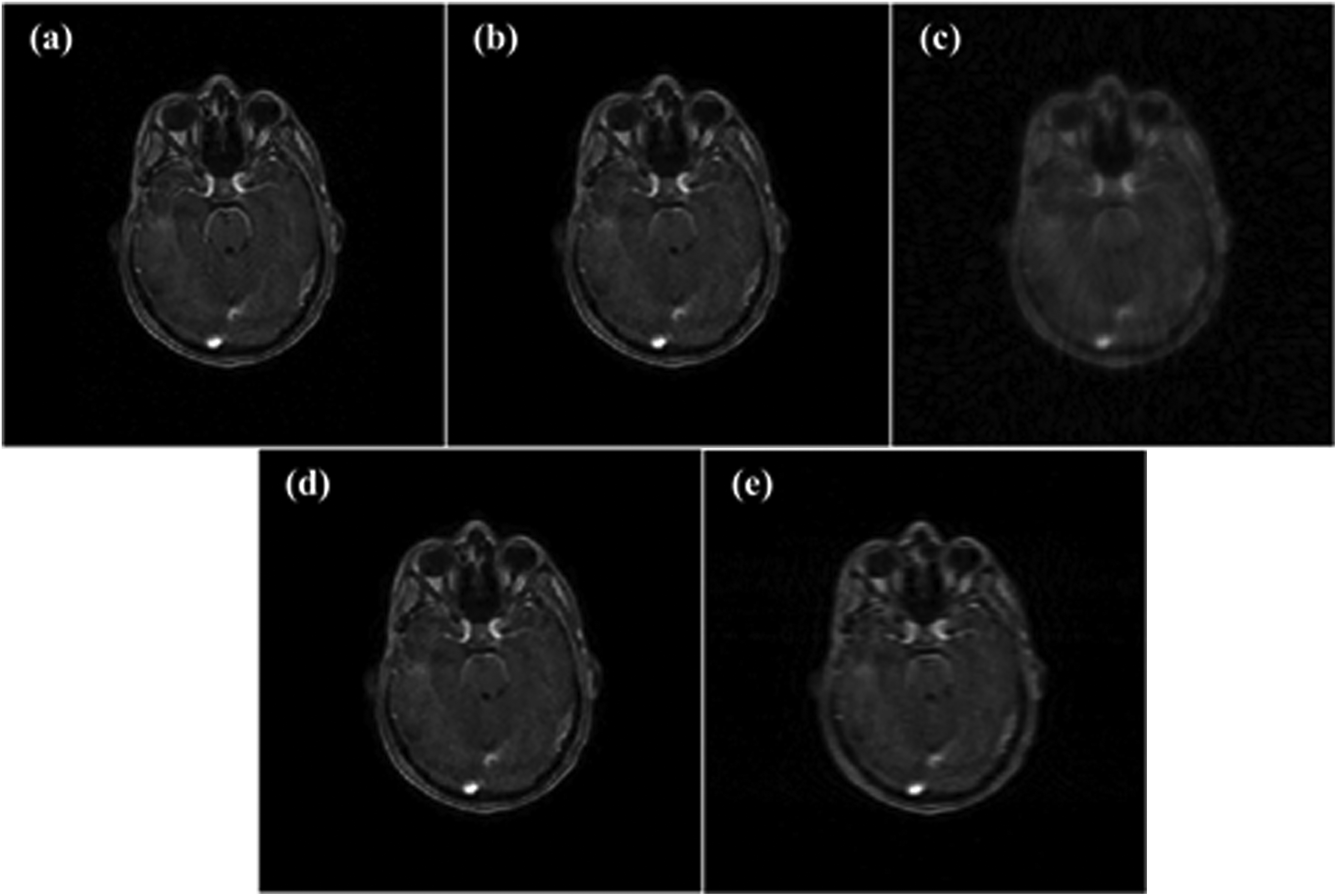
The comparison of undersampled dynamic contrast-enhanced (DCE) image with and without total generalized variation (TGV) reconstruction. A, Reference full-sampled image; (B) TGV-reconstructed image using radial-based undersampling strategy; (C) direct inverse Fourier transform from undersampled data using radial-based undersampling strategy; (D) TGV-reconstructed image using Cartesian-based undersampling strategy; (E) direct inverse Fourier transform from undersampled data using Cartesian-based undersampling strategy.

In a balance of calculation accuracy and efficiency, we limited the maximum iteration step to 8 for DCE image reconstruction in this work, and this choice can be justified by the curves shown in Figure S4 in the supplementary material document. As the average results of 100 reconstructed images from different scans, the blue curve shows the time (in seconds) consumption of each iteration step, and the red curve summarizes the residue (normalized to 100) of the reconstructed images in logarithmic scale at each step. After the eighth step, the blue computation time curve reached a stable plateau, whereas the red residue curve indicated no significant reduction. The total reconstructed time of an image was about 90 seconds.

To improve the PK model fitting quality, an improved texture preserving variational denoising method was applied to the CA concentration maps to reduce the spatial noise effect. The same implementation was adopted for both fully sampled data sets and reduced sampled data sets. In the DCE-MRI acquisition, the image quality may be compromised as the acquisition speed increased. So far, the noise effect in CA concentration maps has not been fully characterized yet. As a typical approach of pixel-by-pixel analysis, the spatial averaging strategy has been reported in various clinical studies for PK analysis.⁷¹ In addition, for certain PK parameters, the spatial filtering was needed to remove the noise effect.⁶⁴ In the denoising method used in this study, the noise reduction was optimized with a spatially varying local power constraint.^59,72 Compared to the classic variational denoising technique and moving average kernel, this method has been reported to improve the image quality in terms of signal-to-noise ratio (SNR) at no change in spatial patterns.^59,73 Defined by the general shape and spatial distribution of a certain biomarker’s map, texture features are independent of the biomarker’s absolute value and are less sensitive to temporal and spatial resolution effects.^74
–76 It has been reported that texture features may have great potentials in monitoring the treatment response as a robust biomarker.⁷⁷ As a future work, it would be interesting to investigate whether texture feature can be accurately reproduced as a robust biomarker with highly accelerated DCE-MRI studies.

In this study, we used the individualized AIF measurement for the PK analysis, and such measurement requires the existence of a major arterial structure within the imaging volume. Due to current technical limit, a limited volume of interest is covered with an adequate spatial resolution at a reasonable temporal resolution, and the lesion has to be close to a major intracranial arterial structure. Unfortunately, this requirement was hard to be satisfied, and thus, only a small number of patients were qualified for this pilot study. We acknowledge that 8 DCE-MRI data sets may not broad enough for a population study, but we think that this feasibility study with these 8 scans would be a good pilot study, and the current work is an early demonstration of the proposed method. Certainly, future works with a much larger number of data sets on various tumors are essential toward the clinical application of the proposed DCE-MRI acceleration method.

The inclusion of individual AIF measurement is an important factor of this work. It has been claimed that characterization of an individual AIF in preclinical studies is very difficult and could be misleading.³⁷ For brain analysis, the AIF extraction based on time-to-peak information has shown its reproducibility in the longitudinal study.⁷⁸ To maintain AIF’s enhancement feature, some studies used only a certain number or percentage of voxels based on the peak enhancement ratio in AIF generation.^60,78 However, such a method is sensitive to the absolute CA concentration value, and the data reproducibility may be reduced when intensity-based image reconstructed methods were used. In this work, we selected a group of voxels based on the time-to-peak distribution and average the resultant time course to create AIF. To ensure the accuracy, this approach requires a large volume of arterial structure to generate a sufficient number of qualified voxels. In practice, however, the requirement was difficult to satisfy. The noise content of the CA concentration curve has been quantified as contrast-to-noise ratio (CNR) that is the ratio of maximum peak to the standard deviation of Gaussian random noise.⁷⁹ The reported CNR value of CA concentration curves ranged from 4 to 20.^64,80 In earlier studies, polynomial filters have been used in the model-free DCE-MRI analysis.⁸¹ For the quantitative PK analysis, the similar filtering strategies may further improve analysis accuracy when using undersampled data, but additional future works are in demand to demonstrate the feasibility of such filtering strategy.

Conclusion

The feasibility of accelerated brain DCE-MRI has been successfully demonstrated in the quantitative PK parameters. As shown in this study, the quantitative parameters from 2 commonly adopted PK models can be accurately calculated from the images reconstructed with 2 data undersampling strategies at a simulated acceleration factor of 4. These results suggested that the investigated acceleration method can be used for reliable clinical image acquisition. Future works with a large population are in demand toward the exploration of this method before routine clinical implementation.

Footnotes

Abbreviations

Acknowledgments

The authors would like to thank Kevin Kelly for his help with DCE-MRI data acquisition. They would also like to thank Dr Ergys Subashi for proofreading the manuscript and for language improvements.

Declaration of Conflicting Interests

The author(s) declared no potential conflicts of interest with respect to the research, authorship, and/or publication of this article.

Funding

The author(s) received no financial support for the research, authorship, and/or publication of this article.

Supplemental Material

The online Supplemental Figures are available at .

References

Hylton

. Dynamic contrast-enhanced magnetic resonance imaging as an imaging biomarker. J Clin Oncol. 2006;24(20):3293–3298. doi:10.1200/Jco2006.06.8080.

Kershaw

Buckley

. Precision in measurements of perfusion and microvascular permeability with T1-weighted dynamic contrast-enhanced MRI. Magn Reson Med. 2006;56(5):986–992. doi:10.1002/mrm.21040.

Choyke

Dwyer

Knopp

. Functional tumor imaging with dynamic contrast-enhanced magnetic resonance imaging. J Magn Reson Imaging. 2003;17(5):509–520. doi:10.1002/Jmri.10304.

Langer

van der Kwast

Evans

Trachtenberg

Wilson

Haider

. Prostate cancer detection with multi-parametric MRI: logistic regression analysis of quantitative T2, diffusion-weighted imaging, and dynamic contrast-enhanced MRI. J Magn Reson Imaging. 2009;30(2):327–334. doi:10.1002/jmri.21824.

Turnbull

. Dynamic contrast-enhanced MRI in the diagnosis and management of breast cancer. NMR Biomed. 2009;22(1):28–39. doi:10.1002/nbm.1273.

Delongchamps

Beuvon

Eiss

. Multiparametric MRI is helpful to predict tumor focality, stage, and size in patients diagnosed with unilateral low-risk prostate cancer. Prostate Cancer Prostatic Dis. 2011;14(3):232–237. doi:10.1038/Pcan.2011.9.

van der Heide

Houweling

Groenendaal

Beets-Tan

RGH

Lambin

. Functional MRI for radiotherapy dose painting. Magn Reson Imaging. 2012;30(9):1216–1223. doi:10.1016/j.mri.2012.04.010.

Yaromina

Krause

Baumann

. Individualization of cancer treatment from radiotherapy perspective. Mol Oncol. 2012;6(2):211–221. doi:10.1016/j.molonc.2012.01.007.

Bauerle

Bartling

Berger

. Imaging anti-angiogenic treatment response with DCE-VCT, DCE-MRI and DWI in an animal model of breast cancer bone metastasis. Eur J Radiol. 2010;73(2):280–287. doi:10.1016/j.ejrad.2008.10.020.

10.

Chang

Wang

. Treatment assessment of radiotherapy using MR functional quantitative imaging. World J Radiol. 2015;7(1):1–6.

11.

Jarnagin

Schwartz

Gultekin

. Regional chemotherapy for unresectable primary liver cancer: results of a phase II clinical trial and assessment of DCE-MRI as a biomarker of survival. Ann Oncol. 2009;20(9):1589–1595. doi:10.1093/annonc/mdp029.

12.

O’Connor

Jackson

Parker

Jayson

. DCE-MRI biomarkers in the clinical evaluation of antiangiogenic and vascular disrupting agents. Br J Cancer. 2007;96(2):189–195. doi:10.1038/sj.bjc.6603515.

13.

Wang

Horton

Yin

Chang

. Assessment of treatment response with diffusion-weighted MRI and dynamic contrast-enhanced MRI in patients with early-stage breast cancer treated with single-dose preoperative radiotherapy initial results [published online July 1, 2015]. Technol Cancer Res Treat. 2015.

14.

Zahra

Hollingsworth

Sala

Lomas

Tan

. Dynamic contrast-enhanced MRI as a predictor of tumour response to radiotherapy. Lancet Oncol. 2007;8(1):63–74. doi:10.1016/S1470-2045(06)71012-9.

15.

Wang

Yin

Horton

Chang

. Review of treatment assessment using DCE-MRI in breast cancer radiation therapy. World J Methodol. 2014;4(2):46–58.

16.

Port

Knopp

Brix

. Dynamic contrast-enhanced MRI using Gd-DTPA: interindividual variability of the arterial input function and consequences for the assessment of kinetics in tumors. Magn Reson Med. 2001;45(6):1030–1038. doi:10.1002/Mrm.1137.

17.

van Osch

MJP

Vonken

EJPA

Viergever

van der Grond

Bakker

CJG

. Measuring the arterial input function with gradient echo sequences. Magn Reson Med. 2003;49(6):1067–1076. doi:10.1002/Mrm.10461.

18.

Henderson

Rutt

Lee

. Temporal sampling requirements for the tracer kinetics modeling of breast disease. Magn Reson Imaging. 1998;16(9):1057–1073.

19.

Wang

Yin

Chang

. An efficient calculation method for pharmacokinetic parameters in brain permeability study using dynamic contrast-enhanced MRI. Magn Reson Med. 2016;75(2):739–749.

20.

Yankeelov

Luci

Lepage

. Quantitative pharmacokinetic analysis of DCE-MRI data without an arterial input function: a reference region model. Magn Reson Imaging. 2005;23(4):519–529. doi:10.1016/j.mri.2005.02.013.

21.

Loveless

Halliday

Liess

. A quantitative comparison of the influence of individual versus population-derived vascular input functions on dynamic contrast enhanced-MRI in small animals. Magn Reson Med. 2012;67(1):226–236. doi:10.1002/mrm.22988.

22.

Parker

Roberts

Macdonald

. Experimentally-derived functional form for a population-averaged high-temporal-resolution arterial input function for dynamic contrast-enhanced MRI. Magn Reson Med. 2006;56(5):993–1000. doi:10.1002/mrm.21066.

23.

d’Arcy

Collins

Padhani

Walker-Samuel

Suckling

Leach

. Informatics in Radiology (infoRAD): Magnetic Resonance Imaging Workbench: analysis and visualization of dynamic contrast-enhanced MR imaging data. Radiographics. 2006;26(2):621–632. doi:10.1148/rg.262045187.

24.

Subashi

Choudhury

Johnson

. An analysis of the uncertainty and bias in DCE-MRI measurements using the spoiled gradient-recalled echo pulse sequence. Med Phys. 2014;41(3):032301. doi:10.1118/1.4865790.

25.

Heisen

Fan

Buurman

van Riel

NAW

Karczmar

Romeny

BMT

. The influence of temporal resolution in determining pharmacokinetic parameters from DCE-MRI data. Magn Reson Med. 2010;63(3):811–816. doi:10.1002/Mrm.22171.

26.

Di Giovanni

Azlan

Ahearn

Semple

Gilbert

Redpath

. The accuracy of pharmacokinetic parameter measurement in DCE-MRI of the breast at 3 T. Phys Med Biol. 2010;55(1):121–132. doi:10.1088/0031-9155/55/1/008.

27.

van Vaals

Brummer

Dixon

. “Keyhole” method for accelerating imaging of contrast agent uptake. J Magn Reson Imaging. 1993;3(4):671–675.

28.

Subashi

Moding

Cofer

. A comparison of radial keyhole strategies for high spatial and temporal resolution 4D contrast-enhanced MRI in small animal tumor models. Med Phys. 2013;40(2):02230 4. doi:10.1118/1.4774050.

29.

Tsao

Boesiger

Pruessmann

. k-t BLAST and k-t SENSE: dynamic MRI with high frame rate exploiting spatiotemporal correlations. Magn Reson Med. 2003;50(5):1031–1042. doi:10.1002/mrm.10611.

30.

Donoho

. Compressed sensing. IEEE Trans Info Theory. 2006;52:1289–1306.

31.

Lustig

Donoho

Santos

Pauly

. Compressed sensing MRI. IEEE Signal Proc Mag. 2008;25(2):72–82. doi:10.1109/Msp.2007.914728.

32.

Lustig

Donoho

Pauly

. Sparse MRI: the application of compressed sensing for rapid MR imaging. Magn Reson Med. 2007;58(6):1182–1195. doi:10.1002/mrm.21391.

33.

Gamper

Boesiger

Kozerke

. Compressed sensing in dynamic MRI. Magn Reson Med. 2008;59(2):365–373. doi:10.1002/mrm.21477.

34.

Jung

Sung

Nayak

Kim

. k-t FOCUSS: a general compressed sensing framework for high resolution dynamic MRI. Magn Reson Med. 2009;61(1):103–116. doi:10.1002/mrm.21757.

35.

Fischer

Breuer

Blaimer

Seiberlich

Jakob

Accelerated dynamic imaging by reconstructing sparse differences using compressed sensing. Paper presented at: ISMRM 16th Scientific Meeting and Exhibition; Toronto, Ontario, Canada: May 3-9, 2008.

36.

Lustig

Santos

Donoho

Pauly

JM.

kt-SPARSE: High frame rate dynamic MRI exploiting spatio-temporal sparsity. In: Proceedings of the 13th Annual Meeting of ISMRM; Seattle, WA, May 6-12, 2006.

37.

Han

Paulsen

Zhu

. Temporal/spatial resolution improvement of in vivo DCE-MRI with compressed sensing-optimized FLASH. Magn Reson Imaging. 2012;30(6):741–752. doi:10.1016/j.mri.2012.02.001.

38.

Wang

Miao

Zhou

. Feasibility of high temporal resolution breast DCE-MRI using compressed sensing theory. Med Phys. 2010;37(9):4971–4981.

39.

Smith

Gambrell

. Robustness of quantitative compressive sensing MRI: the effect of random undersampling patterns on derived parameters for DCE- and DSC-MRI. IEEE Trans Med Imaging. 2012;31(2):504–511. doi:10.1109/TMI.2011.2172216.

40.

Smith

Welch

. Quantitative effects of using compressed sensing in dynamic contrast enhanced MRI. Phys Med Biol. 2011;56(15):4933–4946. doi:10.1088/0031-9155/56/15/018.

41.

Chen

Schabel

DiBella

. Reconstruction of dynamic contrast enhanced magnetic resonance imaging of the breast with temporal constraints. Magn Reson Imaging. 2010;28(5):637–645. doi:10.1016/j.mri.2010.03.001.

42.

Block

Uecker

Frahm

. Undersampled radial MRI with multiple coils. Iterative image reconstruction using a total variation constraint. Magn Reson Med. 2007;57(6):1086–1098. doi:10.1002/Mrm.21236.

43.

Knoll

Bredies

Pock

Stollberger

. Second order total generalized variation (TGV) for MRI. Magn Reson Med. 2011;65(2):480–491. doi:10.1002/Mrm.22595.

44.

Bredies

Kunisch

Pock

. Total generalized variation. Siam J Imaging Sci. 2010;3(3):492–526. doi:10.1137/090769521.

45.

Nagel

Laun

Weber

Matthies

Semmler

Schad

. Sodium MRI using a density-adapted 3D radial acquisition technique. Magn Reson Med. 2009;62(6):1565–1573.

46.

Winkelmann

Schaeffter

Koehler

Eggers

Doessel

. An optimal radial profile order based on the Golden Ratio for time-resolved MRI. IEEE Trans Med Imaging. 2007;26(1):68–76. doi:10.1109/TMI.2006.885337.

47.

Kohler

A projection access scheme for iterative reconstruction based on the golden section. Paper presented at: Nuclear Science Symposium Conference Record; October 16-22, 2004 IEEE:3961–3965.

48.

Tsai

Nishimura

. Reduced aliasing artifacts using variable-density k-space sampling trajectories. Magn Reson Med. 2000;43(3):452–458. doi:10.1002/(Sici)1522-2594(200003)43:3<452::Aid-Mrm18>3.0.Co;2-B.

49.

Kazantsev

Matej

Lewitt

. Optimal ordering of projections using permutation matrices and angles between projection subspaces. Electron Notes Discrete Math. 2005;20:205–216.

50.

Rasche

Boer

RWD

Holz

Proksa

. Continuous radial data acquisition for dynamic MRI. Magn Reson Med. 1995;34(5):754–761.

51.

d’Arcy

Collins

Rowland

Padhani

Leach

. Applications of sliding window reconstruction with Cartesian sampling for dynamic contrast enhanced MRI. NMR Biomed. 2002;15(2):174–183.

52.

Knoll

Clason

Bredies

Uecker

Stollberger

. Parallel imaging with nonlinear reconstruction using variational penalties. Magn Reson Med. 2012;67(1):34–41. doi:10.1002/Mrm.22964.

53.

Hohage

. Logarithmic convergence rates of the iteratively regularized Gauss-Newton method for an inverse potential and an inverse-scattering problem. Inverse Probl. 1997;13(5)1279–1299. doi:10.1088/0266-5611/13/5/012.

54.

Uecker

Hohage

Block

Frahm

. Image reconstruction by regularized nonlinear inversion—joint estimation of coil sensitivities and image content. Magn Reson Med. 2008;60(3):674–682. doi:10.1002/mrm.21691.

55.

Chan

Golub

Mulet

. A nonlinear primal-dual method for total variation-based image restoration. SIAM J Sci Comput. 1999;20(6):1964–1977.

56.

Esser

Zhang

Chan

. A general framework for a class of first order primal-dual algorithms for convex optimization in imaging science. Siam J Imaging Sci. 2010;3(4):1015–1046.

57.

Chambolle

Pock

. A first-order primal-dual algorithm for convex problems with applications to imaging. J Math Imaging Vis. 2011;40(1):120–145. doi:10.1007/s10851-010-0251-1.

58.

Schabel

Morrell

. Uncertainty in T-1 mapping using the variable flip angle method with two flip angles. Phys Med Biol. 2009;54(1):N1–N8. doi:10.1088/0031-9155/54/1/N01.

59.

Gilboa

Sochen

Zeevi

. Texture preserving variational denoising using an adaptive fidelity term. Paper presented at: 2nd IEEE Workshop on Variational, Geometric and Level Set Methods in Computer Vision. Acropolis, Nice, France. October 16, 2003.

60.

Farjam

Tsien

Lawrence

Cao

. DCE-MRI defined subvolumes of a brain metastatic lesion by principle component analysis and fuzzy-c-means clustering for response assessment of radiation therapy. Med Phys. 2014;41(1):01170 8. doi:10.1118/1.4842556.

61.

Yankeelov

Gore

. Dynamic contrast enhanced magnetic resonance imaging in oncology: theory, data acquisition, analysis, and examples. Curr Med Imaging Rev. 2009;3(2):91–107. doi:10.2174/157340507780619179.

62.

Sourbron

Buckley

. On the scope and interpretation of the Tofts models for DCE-MRI. Magn Reson Med. 2011;66(3):735–745. doi:10.1002/mrm.22861.

63.

Murase

. Efficient method for calculating kinetic parameters using T-1-weighted dynamic contrast-enhanced magnetic resonance imaging. Magn Reson Med. 2004;51(4):858–862. doi:10.1002/Mrm.20022.

64.

Sourbron

Ingrisch

Siefert

Reiser

Herrmann

. Quantification of cerebral blood flow, cerebral blood volume, and blood-brain-barrier leakage with DCE-MRI. Magn Reson Med. 2009;62(1):205–217. doi:10.1002/Mrm.22005.

65.

Brix

Kiessling

Lucht

. Microcirculation and microvasculature in breast tumors: pharmacokinetic analysis of dynamic MR image series. Magn Reson Med. 2004;52(2):420–429. doi:10.1002/mrm.20161.

66.

Moré

. Lecture Notes in Mathematics. In: Watson

, ed. Numerical Analysis. Berlin, Germany: Springer; 1978:105–116.

67.

Chang

Xiang

. Highly accelerated MRI by skipped phase encoding and edge deghosting with array coil enhancement (SPEED-ACE). Med Phys. 2006;33(10):3758–3766.

68.

Lebel

Jones

Ferre

Law

Nayak

. Highly accelerated dynamic contrast enhanced imaging. Magn Reson Med. 2014;71(2):635–644. doi:10.1002/mrm.24710.

69.

Zhu

Guo

Lingala

Lebel

Law

Nayak

. GOCART: GOlden-angle CArtesian randomized time-resolved 3D MRI [published online December 18, 2015]. Magn Reson Imaging. 2015.

70.

Zhuo

Haldar

Hwu

Liang

Sutton

. Accelerating iterative field-compensated MR image reconstruction on GPUs. Biomedical Imaging: From Nano to Macro. Paper presented at: 2010 IEEE International Symposium on Biomedical Imaging; April 14-17, 2010; Rotterdam, The Netherlands:820–823.

71.

Cabrera

Cuneo

Desjardins

. Concurrent stereotactic radiosurgery and bevacizumab in recurrent malignant gliomas: a prospective trial. Int J Radiat Oncol. 2013;86(5):873–879. doi:10.1016/j.ijrobp.2013.04.029.

72.

Blanc-Féraud

Charbonnier

Aubert

Barlaud

Nonlinear image processing: modeling and fast algorithm for regularization with edge detection. In Proceedings of International Conference on Image Processing; Crystal City, TX, USA, October 23-26, 1995: 474–477. IEEE, 1995.

73.

Buades

Coll

Morel

. A review of image denoising algorithms, with a new one. Multiscale Model Sim. 2005;4(2):490–530. doi:10.1137/040616024.

74.

Haralick

Shanmuga

Dinstein

. Textural features for image classification. IEEE T Syst Man Cyb Smc. 1973;3(6):610–621. doi:10.1109/Tsmc.1973.4309314.

75.

Holli

Lääperi

A-L

Harrison

. Characterization of breast cancer types by texture analysis of magnetic resonance images. Acad Radiol. 2010;17(2):135–141.

76.

Alic

Veenland

van Vliet

Van Dijke

Eggermont

Niessen

WJ.

Quantification of heterogeneity in dynamic contrast enhanced MRI data for tumor treatment assessment. Paper presented at: 3rd IEEE International Symposium on Biomedical Imaging: Nano to Macro; April 6-9, 2006: 944–947.

77.

Alic

van Vliet

van Dijke

Eggermont

Veenland

Niessen

. Heterogeneity in DCE-MRI parametric maps: a biomarker for treatment response? Phys Med Biol. 2011;56(6):1601–1616. doi:10.1088/0031-9155/56/6/006.

78.

Parker

Jackson

Waterton

Buckley

. Automated arterial input function extraction for T1-weighted DCE-MRI. In: Proceedings of the 11th Annual Meeting of ISMRM; July 10-16, 2003, Toronto, Canada. 1264.

79.

Luypaert

Sourbron

Makkat

de Mey

. Error estimation for perfusion parameters obtained using the two-compartment exchange model in dynamic contrast-enhanced MRI: a simulation study. Phys Med Biol. 2010;55(21):6431–6443. doi:10.1088/0031-9155/55/21/006.

80.

Cao

Shen

Normolle

. Sensitivity of quantitative metrics derived from DCE MRI and a pharmacokinetic model to image quality and acquisition parameters. Acad Radiol. 2010;17(4):468–478. doi:10.1016/j.acra.2009.10.021.

81.

Jesberger

Rafie

Duerk

. Model-free parameters from dynamic contrast-enhanced-MRI: sensitivity to EES volume fraction and bolus timing. J Magn Reson Imaging. 2006;24(3):586–594. doi:10.1002/jmri.20670.

Supplementary Material

Please find the following supplemental material available below.

For Open Access articles published under a Creative Commons License, all supplemental material carries the same license as the article it is associated with.

For non-Open Access articles published, all supplemental material carries a non-exclusive license, and permission requests for re-use of supplemental material or any part of supplemental material shall be sent directly to the copyright owner as specified in the copyright notice associated with the article.

0.00 MB

1.24 MB