The proteomics and interactomics of human erythrocytes

Abstract

In this minireview, we focus on advances in our knowledge of the human erythrocyte proteome and interactome that have occurred since our seminal review on the topic published in 2007. As will be explained, the number of unique proteins has grown from 751 in 2007 to 2289 as of today. We describe how proteomics and interactomics tools have been used to probe critical protein changes in disorders impacting the blood. The primary example used is the work done on sickle cell disease where biomarkers of severity have been identified, protein changes in the erythrocyte membranes identified, pharmacoproteomic impact of hydroxyurea studied and interactomics used to identify erythrocyte protein changes that are predicted to have the greatest impact on protein interaction networks.

Keywords

Erythrocyte red blood cell proteomics proteome interactomics sickle cell disease

Introduction

Over five years ago we published, in this journal, the first review written on the erythrocyte proteome including the first attempts to look at the red blood cell interactome and how it changes in the case of sickle cell disease (SCD).¹ At that time, there had been 751 unique proteins that were demonstrated to be part of the erythrocyte proteome based on studies from several laboratories including our own.^2–5 Today, that number stands at 2289 proteins, and several computational and mathematical techniques have been utilized to understand the resulting interactome and how it is impacted by proteomic changes in blood disorders such as SCD. In this minireview, we summarize the advances over the period of 2007–2012 in both the proteomics and interactomics of the human erythrocyte and how they are impacted by SCD. The aim of the study was to give our view of the flow of this field and, due to the page and reference limitations of a minireview, it will not be an exhaustive review of the entire literature on this subject. We apologize in advance to numerous authors of articles that we will not be able to discuss or reference and refer the reader to several reviews that followed our seminal review, on this subject.^6–16

Advances in erythrocyte proteomics

The erythrocyte proteome in 2007 had 751 unique proteins.¹ We listed them in a table and produced the very first erythrocyte interactome maps which included a repair or destroy (ROD) box that contained a dense set of interconnected and clustered nodes, including proteasomal, chaperonin and heat shock proteins.¹ The presence of proteasomes in mature erythrocytes, first suggested by proteomic studies,³ was confirmed when Neelam et al. recently demonstrated functional 20 S proteasomes within these cells.¹⁷ The 751 proteins listed came primarily from three studies, each of which brought sequential improvements in methodology and/or technology over the previous one. Low et al. ² in 2002 used a two-dimensional IEF-SDS PAGE followed by in gel trypsin digestion and MALDI TOF mass spectrometry (MS) and looked only at erythrocyte membrane proteins. They identified 84 unique proteins. Our own study followed in 2004 and used a well-established set of cell biological approaches to expose various membrane surfaces and membrane skeletal proteins, as well as separating cytosolic proteins by gel filtration, prior to digestion with trypsin in solution.³ We then utilized reverse phase HPLC coupled to a ThermoFinnigan LCQ DECA XP Ion Trap Tandem MS to identify proteins. The result of this next step up in methodology and technology was the identification of 181 unique membrane and cytosolic proteins. The third study in 2006 was by Pasini et al.⁴ in which the jump in proteins identified was based on the availability of more sensitive technology. They used a similar methodology to that used by Kakhniashvili et al.,³ but coupled it to very sensitive and accurate mass spectrometers which had become commercially available (Applied Biosystems Quadropole TOF Q-STAR MS and a Thermo Electron hybrid linear ion trap Fourier transform MS with sensitivity down to attomoles and accuracy to 1 ppm).⁴ The result was identification of 566 unique membrane and cytosolic proteins.⁴ In total, these three studies led to the 751 proteins known to be in the erythrocyte proteome in 2007, which represent one-third of the proteins known to be part of the proteome today (Figure 1).¹

Figure 1

Growth of our knowledge of the erythrocyte proteome from 2002 to 2012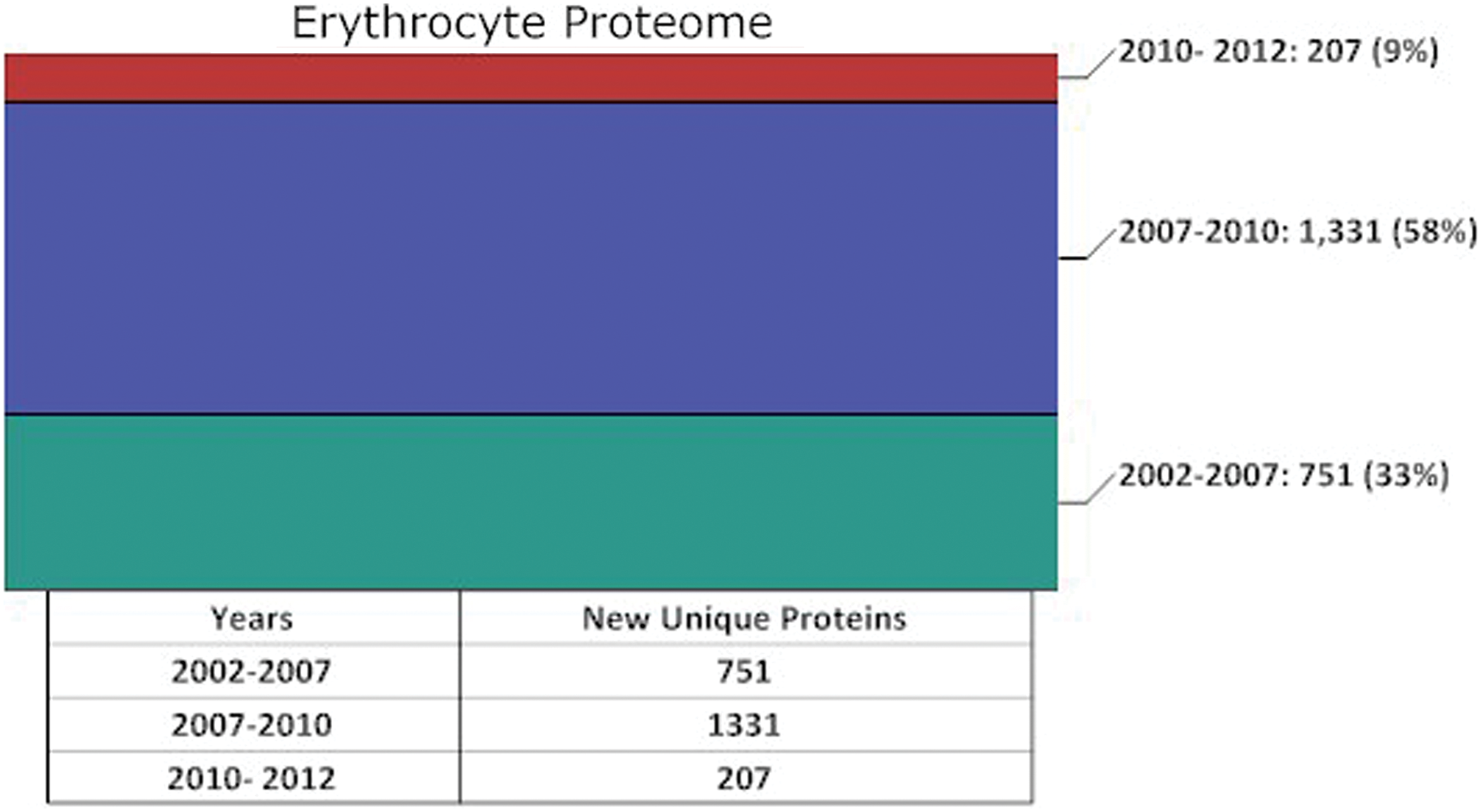

Within one year of the publication of our initial review on this subject, published in Experimental Biology and Medicine, the number of proteins within the erythrocyte proteome had more than doubled to greater than 1800. The greatest jump in the number of erythrocyte proteins within the proteome between 2007 and the end of 2008 was in our knowledge of cytosolic proteins. This growth had been due to a new methodology being applied to the erythrocyte proteome: peptide ligand library and advanced MS.^18–21 Using two different combinatorial libraries of hexapeptides in series, and a Thermo Electron LTQ Orbitrap MS, Roux-Dalvai et al. were able to decrease the dynamic range in solution between the most and least prominent proteins and identify 1578 cytosolic proteins.²⁰ An interesting update of our review by D’Alessandro et al.¹² which was published in 2010 included proteomic studies published after the submission of our review.¹ These studies included the analysis by the combinatorial library Proteominer Technology^18–21 and studies on stored blood,^22–24 and in total the erythrocyte proteome stood at 1989 distinct gene products in this review.¹² Interestingly, D'Alessandro and colleagues interactive network analysis of this larger database of erythrocytes proteins confirmed the central role that the ROD box¹ plays in maintaining cellular homoeostasis in the face of oxidative stress and added the possibility that the ROD box proteins are functioning as a catalytic ring.¹² The total number of unique erythrocyte proteome proteins based on our analysis of the literature stood at 2082 by the end of the period (Supplementary Table 1 and Figure 1) summarized by D’Alessandro et al.¹² This increase in 1331 proteins represented 58% of the erythrocyte proteome known today and was largely due to the combinatorial library Proteominer Technology expanding our understanding of the erythrocyte cytosolic protein complement (Figure 1).

What has been accomplished between 2010 and today in expanding our knowledge of the erythrocyte proteome? During the past three years, the growth in our knowledge of the human erythrocyte proteome has been mainly in the area of the membrane proteins. The challenges concerning the mining of membrane proteins are well known and chronicled,²⁵ and relate to high hydrophobicity and isoelectric point of many transmembrane integral membrane proteins, and heavy glycosylation and the low copy of some.

During the past three years since the review by D’Allesandro et al.,¹² there have been several important technical advances that have uncovered new membrane proteins. van Gestel et al., by using a two-dimensional blue-native PAGE which separates protein complexes followed by SDS PAGE, were able to see 150 protein spots, from an RBC membrane preparation, which led to the identification of 524 proteins of which only 67 were cytosolic.²⁶ More recently, this approach has been expanded to a four-dimensional orthogonal electrophoresis system which includes non-denaturing thin layer IEF followed by native-PAGE, to separate protein complexes, followed by denaturing IEF and SDS PAGE to separate individual proteins.²⁷ This approach allowed the proteomic identification of proteins in six different complexes, the 20 S proteasome, haemoglobin α2β2, haemoglobin α2δ2, carbonic anhydrase, heat shock protein-60 and peryoxiredoxin-2.²⁷ De Palma et al.²⁸ starting with erythrocyte membranes first performed trypsin digestion of intact cells, as Kakhniashvili et al. had done,³ then isolated membranes, solubilized in triton X-100, separated a soluble fraction and a skeletal pellet and trypsin digested both. Each of the three fractions of tryptic peptides were then separated by multidimensional protein identification technology (MudPIT) and then analysed on a linear ion trap LTQ MS. The result was identification of 299 unique proteins of which 211 were identified as being from the membrane.²⁸ Recently, Speicher and colleagues²⁹ have separated erythrocyte membrane proteins by 1D SDS PAGE and found that when they cut the gels into 30 uniform slices, and performed in gel digestion of each, they were able to identify 842 unique proteins utilising an LTQ-Orbitrap XL MS. This is interesting as Bosman et al. by using the same 1D SDS PAGE approach with a 7 T linear quadrupole ICR-FT MS identified 257 unique proteins in 2008.²² Apparently, the critical difference was that Bosman et al. cut their gels into six segments²² while Pesciotta et al. utilized 30 slices.²⁹ Bosman et al. by studying the proteome of various age erythrocytes and microparticles isolated from plasma identified 271 proteins in the erythrocyte membranes and 71 proteins in the erythrocyte-derived microparticles.²³

While the studies listed above have been impressive in applying creative proteomic approaches to identifying erythrocyte membrane proteins, the end result is that the erythrocyte proteome grew from 2082 proteins in 2010 (Figure 1) to 2289 proteins today (see Figure 1 and Supplementary Table 1 which provides the entire list with gene codes). The growth of unique proteins within the erythrocyte proteome was only 207 from 2010 to 2012 which represents 9% of our currently identified erythrocyte proteome (Figure 1). This means that either we are nearing the end of the mining of the erythrocyte proteome or that we now must await the next improvements of mass spectrometers with even higher sensitivity and accuracy to mine for those proteins which are present in one to one hundred copy numbers. It is possible that both are true. We believe that there is more work to be done on the low copy number erythrocyte proteome.

Probably the greatest advances over the past three years is the application of our knowledge of the normal erythrocyte proteome and interactomics to gain a better understanding of the molecular basis, identification, severity and stage of disease, and the effect of various therapeutic drugs upon the erythrocyte proteome. While great advances have been made in SCD (discussed next), there has also been major advances in our understanding of proteomic changes in the erythrocyte membrane in malaria,^30–36 various hemolytic anaemias^37–41 and haemoglobinopathies,^1,42,43 cell storage and aging,^44–47 Alzheimer’s disease,⁴⁸ schizophrenia,^49–51 chronic pulmonary disorder,⁵² chronic kidney disease⁵³ and diabetes.^54,55

Sickle cell disease

SCD was the first genetic disorder where the precise molecular basis was understood at the protein level. It is an autosomal recessive disorder where the inheritance of two defective β-globin genes results in homozygous sickle cell (SS) disease. Adult haemoglobin is a α₂β₂ tetramer, and in SCD the α subunits are normal. A point mutation in the β-globin gene on chromosome 11, thymine replaces adenine and causes the single amino acid substitution of valine for glutamic acid in the sixth residue of β-globin. This single amino acid substitution in β-globin creates a sickle cell hemoglobin (HbS) molecule which polymerizes into a 14 stranded polymer when in its deoxy state and depolymerizes when it is well oxygenated. The polymerization of HbS causes the characteristic sickled shape and the polymerization depolymerization cycle leads to reversibly sickled SS erythrocytes. SS subjects also have dense irreversible sickled cells (ISCs) which remain sickled even when HbS is in its oxygenated depolymerized form. First, we will discuss changes in the erythrocyte membrane skeleton, which lead to the ISC, and then the process of vasooclusion, as a prelude to the discussion of the use of proteomics in understanding SCD (review^1,56).

We demonstrated that reversible oxidative damage to actin and diminished ubiquitination of spectrin leads to ISC.^57–65 The formation of a disulphide bridge between Cys 284 and Cys 373 in β-actin leads to an actin filament that will not depolymerize at 37℃.^57–59 Goodman and colleagues have demonstrated that spectrin is a chimeric E2/E3 ubiquitin ligase which can ubiquitinate itself and several other membrane skeletal proteins.^66–70 Spectrin’s E2/E3 ubiquitin conjugating/ligating activity is diminished in SCD with the result being 50–90% decrease in α-spectrin ubiquitination in repeat units 20/21.^62,65 We further demonstrated that ubiquitination regulates the dissociation of the spectrin-4.1-actin⁶² and spectrin–adducin–actin ternary complex,⁶³ and that reduced ubiquitination leads to ternary complexes that dissociate poorly at 37℃.^62,63,71 We demonstrated that antioxidants that raise the reduced glutathione levels within RBCs can block the formation of dense ISCs in vitro and in vivo.^72,73 Our phase 2 human trial with n-acetyl-cysteine demonstrated a 60% reduction in SS crisis rate, at 2400 mg/day, with no obvious side-effects.⁷³

The pathophysiology of SCD is primarily caused by vasoocclusion of the circulatory system leading to impaired oxygen delivery to cells, tissues and organs. Vasoocclusion leads to the painful SS crises or vasoocclusive episodes, which in turn are correlated to the survival of the SS patient. (review^1,56) Vasoocclusion is caused based on changes in erythrocytes, white blood cells, platelets and plasma factors causing these diverse cells to associate with each other and the blood vessel endothelial cells resulting in clogging of the circulatory system. Reversible sickled cells tend to be adhesive to themselves, white blood cells and the blood vessel endothelium, while the ISCs become trapped in the narrowing passage way of blood vessels and capillaries. There is a 15-year difference in 50% survival probability between those SS subjects with one or fewer SS crises per year (mild) versus three or greater crises per year (severe). So, despite SCD being caused by a single point mutation in the β-globin locus of chromosome 11, there is great variability is SS severity and outcome between homozygous SS patients (review^1,56).

Proteomics and interactomics have been and will continue to be used to answer many important questions in SCD. What protein changes exist on the membrane and cytosol of erythrocytes, leukocytes and blood vessel endothelial cells in SS patient versus control blood? What changes occur in the plasma in SCD versus control blood? What changes occur in these cells and plasma when patients or their blood are treated with various drugs? (This is the subject of pharmaco-proteomics.) Can we define biomarkers in erythrocytes, leukocytes, blood vessel endothelial cells or plasma that can reliably predict SS severity? If this is possible, then we will have made available personalized medicine for SCD. We are pleased to report that we have made substantial progress in all of these areas, but there is a long road left to travel.

We performed the first protein profiling on SS versus control RBC membrane protein using the two-dimensional difference gel electrophoresis (2D DIGE) technique and tandem MS.⁷⁴ Of the 500 fluorescent spots studied approximately, 49 changed by at least 2.5 fold when comparing SS versus control (AA) erythrocyte membranes. Thirty-eight proteins increased and 11 decreased by 2.5 fold or greater. The 38 analysed spots yielded 44 protein forms with their modifications and 22 unique proteins. When considering the 22 unique proteins, they fell into a few functional categories: membrane skeletal (actin accessory proteins), protein repair participants, lipid raft components, protein turnover components, scavengers of oxygen radicals and other categories. Interestingly, the results indicated that lipid raft components (stomatin and flotillin) are diminished >2.5 fold in SS RBC membranes, while proteins involved in an adaptive response to oxidative stress were increased by >2.5 fold in SS RBC membranes (heat shock protein subunits, chaperonin subunits, proteasomal subunits, peroxyredoxin and catalase). The protein that changes to the greatest extent was Heat Shock 70 KDa protein 8 subunit 1.

We followed this 2D DIGE study with a proteomic study on SS versus AA core membrane skeletal proteins using cleavable isotope-coded affinity tags (cICAT) which label cysteine residues. We demonstrated that the method variation was 14.1% in log ratios and the variation of the sample population was 13.8% in log ratios, so the calculated total variation in log ratios is 19.7%. Neither α-spectrin, β-spectrin, β-actin or protein 4.1 varied from a ratio of 1 in SS versus AA skeletal proteins.⁷⁵ Therefore, while the cICAT method detects no change in total spectrin, 4.1 or actin,⁷⁵ the 2D DIGE method which can separately detect post-translational modifications (PTMs) and alternate splice forms did demonstrate changed amounts of the modified forms.⁷⁴ As an example, protein 4.1 can be found in 11 discrete spots on the 2D IEF-SDS-PAGE gel and seven of these spots either increase (six spots) or decrease (one spot).⁷⁴ Therefore, when taking these two methods together, protein 4.1 does not change in total content in SCD versus AA erythrocyte membranes, but specific modified forms are changing. If the modifications alter binding affinities or capacity, then interactions in the membrane skeleton will be changing.

Towards the goal of identifying protein biomarkers that can predict SS severity, we conducted protein profiling studies on erythrocytes, leukocytes and plasma derived from patients with known five-year crisis rates or Acute Chest syndrome rates. Our initial success has come in 2D DIGE studies on monocytes. First, we wanted to look at the protein variance in the monocyte proteome in control populations⁷⁶ before moving on to SS versus reference controls.⁷⁷ Using isolated membrane and cytoplasmic fractions from highly purified monocytes isolated from 18 healthy individuals, we performed 2D DIGE experiments.⁷⁶ We studied ∼900 fluorescent protein spots and identified 31 cytosolic and 12 membrane proteins that had the greatest person to person variability in this control population. Twenty-seven cytoplasmic proteins and nine membrane proteins were identified by trypsin digestion and tandem MS. Of the cytosolic proteins, enolase-1 and WD (tryptophan-aspartate) repeat containing protein 1 demonstrated the largest standard deviations (SD). In the membrane fraction, the largest SD was observed for lamin B1 and l-plastin.⁷⁶ Having demonstrated the variability of monocyte proteome content in control populations,⁷⁶ we were now ready to move on to the question of whether we could determine biomarkers for SS severity by comparing the monocyte proteome from individual SS subjects versus a reference control utilizing 2D DIGE. By studying 10 individuals with homozygous SCD (SS) versus a reference control and plotting the number of painful vasoocclusive episodes (crises)/year over five years versus the fluorescent spot log ratio (sample versus reference control), we found that 21 of approximately 1000 protein spots had significant positive or negative correlation based on multivariate statistical analysis. Trypsin digestion and tandem mass spectrometry allowed us to identify these potential biomarkers of SS severity. Based on our studies, the most negatively correlated proteins in the membrane fraction were transketolase and coronin. The most negatively correlated in the cytosolic fraction were heat shock protein cognate 4 and adenylate kinase isoenzyme 2, mitochondrial. The most positively correlated in the cytosolic fraction were far upstream element-binding protein and alpha actinin 1 or 4. Using a sophisticated StepSIM analysis vinculin, leukotriene A-4 hydrolase and phosphoglycerate kinase were all highly predictive of SS vasoocclusive crisis rate. These results are very promising that we are close to having protein biomarkers to SS severity and, therefore, personalized medicine for SCD.⁷⁷ The studies that must follow are validation with a larger sample size of SS subjects and then longitudinal studies beginning two weeks after birth where we can see how early in life the verified biomarkers are predictive of downstream SS severity. In more recent studies, we have moved away from cICAT labelling to isobaric tags for relative and absolute quantitation (iTRAQ) reagents to label amines versus cysteines getting better coverage of any individual protein without the problems of oxidative alterations of cysteines. This multiplexing approach will be utilized in these longitudinal studies as eight samples can be simultaneously compared.

Studies on the plasma of subjects with SCD with or without accompanying pulmonary hypertension (PH) have indicated that decreased apolipoprotein A-I (apoA-I) is a potential marker for PH risk.⁵⁶ Further, the same laboratory has demonstrated that elevation of the serum amyloid A/apoA-I ratio in plasma could be a marker for increased crisis rate.⁵⁶

These same protein profiling approaches are being used to study the proteomic changes induced by drug therapies, and this is referred to as pharmaco-proteomics. Hydroxyurea (HU) raises fetal haemoglobin levels leading to a milder version of SCD. However, substantial evidence exists that it also affects mean cell volume (MCV), reduced SS adhesion to the endothelium and increased deformability of SS erythrocytes (review^1,56). We therefore performed pharmaco-proteomic studies on the impact of HU upon the SS erythrocyte proteome utilizing the 2D DIGE protein profiling methodology and tandem MS.⁷⁸ We demonstrated that when SS erythrocytes were incubated with a clinically relevant concentration of HU, we saw PTMs of the following functional categories of proteins: antioxidant enzymes (catalase, peroxyredoxins), oxidoreductases (aldehyde dehydrogenase), protein repair participants (human T complex protein delta subunit, chaperoning containing TCP 1 subunit 7), protein degradation machinery (proteasome alpha 2 subunit variant), CO₂ conversion (carbonic anhydrase I and II), membrane skeletal protein (p55) and haemoglobin (beta subunit). In the case of catalase, we demonstrated that the increase in acidic forms was due to phosphorylation of tyrosine residues.⁷⁸ This in vitro study was then followed with an in vivo determination of HU-dependent changes in protein expression in SS subjects.⁷⁹ We again used 2D DIGE to perform protein profiling studies on erythrocytes membranes from five SS subjects that had received HU treatment at 30–38 mg/kg/day, for a minimum of seven months, versus a reference control from five SS subjects who had not received HU.⁷⁹ The results indicated increases in expression of multiple modified forms of membrane proteins (band 3, protein 4.1, ankyrin, actin, tropomodulin, stomatin and p55) and glycolytic enzymes (glyceraldehyde 3-phosphate dehydrogenase and fructose-bisphosphate aldolase) and decreases in chaperonin containing TCP1 subunit 2 and proteasome subunit alpha type 4. Only palmitoyalated membrane protein (p55) was increased in both in vitro and in vivo studies. In the in vivo studies where altered expression can indicate increased synthesis and/or PTM in erythropoetic cells or PTMs in the mature erythrocytes, the increased p55 expression in SCD patients receiving HU was five to 10 fold higher than SCD subjects not being treated with HU.⁷⁹ A study with a larger number of SCD patients on HU versus not treated with HU will be of interest to determine whether p55 increases are important in the improved clinical status for SCD subjects being treated with HU.

We refer the reader to other reviews on the proteomics of SCD.^43,56

Interactomics

As biologists keep discovering new RBC proteins and protein interactions from wet lab experiments, mathematicians and computer scientists, on the other hand, provide efficient computational methods so that the newly obtained data can be interpreted accurately and efficiently. Furthermore, wet lab experiments are expensive and time consuming, and thus the importance of obtaining results by efficient and relatively inexpensive computational methods cannot be stressed enough.

A key step in analysing interactomics data is constructing a protein–protein interaction (PPI) network. The foundations of PPI networks lay in the graph theory, one of the core subjects in theoretical computer science. Formally, a graph G is an ordered pair (V(G), E(G)) consisting of a set of nodes and a set of edges, V(G) and E(G), respectively, with an incidence function that associates each edge of G with a pair of (not necessarily distinct) nodes of G. A graph is said to be weighted if a numerical value is associated with each edge in the graph. In the case of PPI networks, proteins are represented by nodes, and if two proteins are known to interact they are connected by an edge. Edge weights denote the probability that the corresponding two proteins will interact. The process of building a PPI network has two major steps: identifying the list of proteins experimentally and discovering their interactions from available interaction databases. RBC interactions from the papers we analyse in this review are obtained from Unified Human Interactome Database (UniHI). Each interaction is assigned the Spearman correlation coefficient, derived from gene expression data, which represents the confidence level of the interaction. Unfortunately, databases such as UniHi contain a number of false positives and false negatives. False positives are interactions that are listed in a database but are non-existent in the real world, while false negatives are existing interactions omitted from the database. In our case, in order to reduce the chance of a false positive interaction being listed, researchers introduced a threshold and all interactions with Spearman coefficient below the threshold of 0.3 are left out.

Once a PPI network is constructed, follow-up steps include utilizing computational methods to analyse the network. Due to the fact that PPI analysis is a broad field and beyond the scope of this review, we only focus on the methods that have been used for the RBC PPI network. Those methods include: centrality measures, Voronoi diagram for graphs and Ingenuity pathway/network analysis.

Centrality measures⁸⁰ was the first computational approach that was utilized in analysing the RBC PPI network and the impact SCD has on it. The idea was to apply a method that was used in social network analysis to a biological network. Centrality measures mainly comprise three parameters that are used to predict the ‘importance’ of a node in a given network, which are as follows: degree centrality, closeness centrality and betweenness centrality. Degree centrality is arguably the simplest and the most intuitive of the three. It represents the number of edges a particular node is incident to. In a PPI network, in particular, it represents the number of interacting partners for a given protein. Degree centrality is fast and easy to compute, but it considers only individual nodes and not the network as a whole. Therefore, some discrepancies in results could occur. For instance, a node with a high degree centrality can still be disconnected from major parts of the network. Closeness centrality measures how close a given node is to all other nodes in the network. Formally, it is the inverse of the average length of all shortest paths from the node of interest. Consequently, nodes with low closeness centrality take small amount of time to propagate through the network. Furthermore, this measure is more accurate than degree centrality as it considers the relationship between the node and the entire network. Betweenness centrality is the ratio between the number of shortest paths going through a vertex and the total number of existing shortest paths in the network. Unfortunately, centrality measures algorithms are slow when it comes to worst case scenarios. It takes O(|V²|) to compute degree centrality and O(|V³|) to compute closeness and betweenness centrality, where |V| denotes the number of nodes in the network. Moreover, although centrality measures give us a notion of which nodes have the highest impact in the network, they do not provide any information regarding the vertices being impacted by a particular node, which is extremely important in the RBC/SCD study as we want to know which proteins will be impacted by a particular SCD altered protein.

Kurdia et al. ⁸⁰ built the RBC PPI network based on the list of 751 RBC proteins which was the most comprehensive list at the time when that paper was written. They found that only 279 of the 751 proteins were actually interacting with other proteins. They identified a large cluster of 229 proteins which included a few nodes that scored high on all centrality measures (see Table 1). Of the 10 proteins that had the highest centrality scores for each form of centrality measurement nine were chaperonin, proteasomal and antioxidant proteins found within the ROD Box (Table 1). Only ankyrin (ank1), the protein which ties spectrin to the cytoplasmic surface of the erythrocyte membrane, is outside the ROD box.

Table 1

SCD-altered protein ranking according to degree, closeness and betweenness centrality measures

Rank	Proteins – degree centrality	Degree centrality value	Proteins – closeness centrality	Closeness centrality value	Proteins – betweenness centrality	Betweenness centrality value
1	PSMC6	38	PSMC6	0.338	PSMC6	0.139501
2	PSMA1	31	CCT6A	0.333	CCT6A	0.120295
3	PSMB1	27	PSMA1	0.313	PRDX1	0.067702
4	CCT6A	22	CCT2	0.310	PSMA1	0.055607
5	CCT2	18	PSMB1	0.305	CCT2	0.046178
6	PRDX1	10	PRDX1	0.285	PSMB1	0.027321
7	CCT4	7	CCT4	0.284	HSPA8	0.017621
8	CCT7	5	HSPA8	0.267	CCT4	0.011747
9	ANK1	3	CCT7	0.265	CCT7	0.008811
10	HSPA8	3	TUBA6	0.246	TUBA6	0.008811

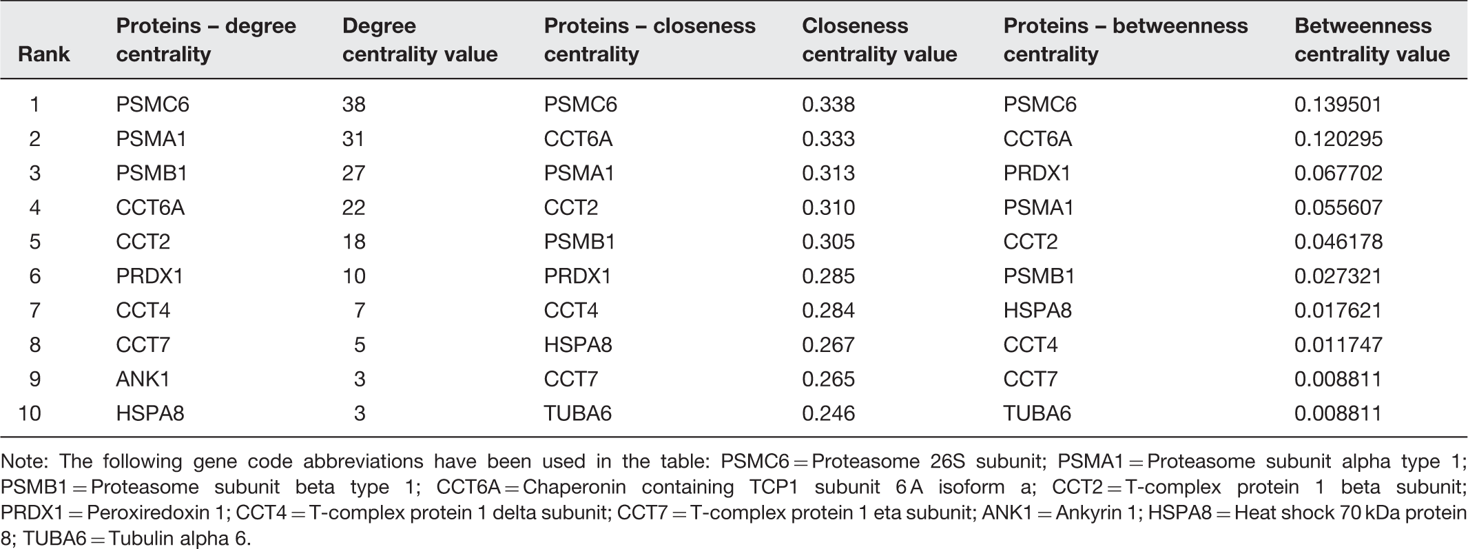
Note: The following gene code abbreviations have been used in the table: PSMC6 = Proteasome 26S subunit; PSMA1 = Proteasome subunit alpha type 1; PSMB1 = Proteasome subunit beta type 1; CCT6A = Chaperonin containing TCP1 subunit 6 A isoform a; CCT2 = T-complex protein 1 beta subunit; PRDX1 = Peroxiredoxin 1; CCT4 = T-complex protein 1 delta subunit; CCT7 = T-complex protein 1 eta subunit; ANK1 = Ankyrin 1; HSPA8 = Heat shock 70 kDa protein 8; TUBA6 = Tubulin alpha 6.

Ammann and Goodman⁸¹ utilized statistical cluster analyses to measure the similarity of nodes within a network a method called Generalized Topological Overlap Measure (GTOM). Using Agnes (agglomerative nesting) for GTOM 1, we demonstrated that multiple SCD altered proteins in the ROD Box group: proteasomal subunits and chaperonins fell within large clusters 1 and 4. Using Diana (divisive analysis) on GTOM 1, we demonstrated that the largest cluster 1 contains the proteasomal subunits altered in SCD.⁸¹ As the Ammann and Goodman article⁸¹ was submitted prior to the appearance of the combinatorial library study by Roux-Dalvai et al.,²⁰ like Kurdia et al.,⁸⁰ it relied upon the erythrocyte proteome 751 proteins described by Goodman et al.¹

In an effort to continue RBC interactome analysis and enhance methods used in Kurdia et al.⁸⁰ and Ammann and Goodman,⁸¹ Zivanic et al.⁸² proposed the use of Voronoi diagram for graphs (VDG). The Voronoi diagram is a distance-based decomposition of a metric space relative to a discrete set S of Voronoi sites. Each Voronoi site determines a Voronoi region, which is a set of points that are closer to that site than to any other site. The common boundary of two Voronoi regions is called a Voronoi edge, and two Voronoi edges meet at a Voronoi vertex. VDG is a generalization of the Voronoi diagram and was proposed by Erwig.⁸³ VDG provides an efficient way to cluster nodes in the network based on their distance to the members of a predetermined subset of cluster centres called Voronoi sites. Formally, let G = (V, E, w) be a graph, where V denotes the nodes, E denotes the edges and w is a weigh function that assigns a weight w > 0 to each edge in E. The VDG for G and a subset K = {v₁, v₂, … , v _k ) of V is a partition Vor(G,K) such that for each node u of V, d (u, v_i) ≤ d(u, v_j) for all j = 1, … , k, where d(u,v) is the shortest path distance between the nodes u and v. If a node is equidistant from multiple cluster centres, it is assigned to all corresponding clusters. The running time of the VDG algorithm is O(|E|) in an unweighted graph, and O(|E| + log |V|) in a weighted graph. This turned out to be the most suitable approach for the study of the RBC interactome and its relationship with SCD. SCD altered proteins serve as cluster centres. Proteins belonging to the same cluster are more likely to be affected by the corresponding SCD-altered protein than any other SCD-altered protein, which was not the case with the centrality measures approach. Furthermore, VDG is much faster than centrality measures and clustering algorithms.

Zivanic et al.⁸² compiled a list of 1834 proteins by assembling data from Roux-Dalvai et al.²⁰ and Goodman et al.¹ After excluding proteins with no interaction and applying the Spearman correlation threshold, the number of proteins dropped to 829 and those were used to create the PPI network. Of the 22 SCD altered proteins, 16 proteins were present in that network implying that the resulting VDG clustering will yield 16 clusters. They consider both the unweighted and the weighted network. In the unweighted network, the distance between any two nodes is represented by the number of edges on the shortest path between those two nodes. In the weighted network, the edge weight is set equal to the confidence level for the interaction between the corresponding two proteins. The distance between any two edges is equal to the product of the edge weights on the shortest path between the two nodes. Figure 2 illustrates the results obtained by Zivanic et al.⁸² where again the chaperonin, proteasomal and antioxidant proteins altered in SCD were all part of major clusters while the ANK1 cluster is small and disconnected from the rest (Figure 2).

Figure 2

Voronoi regions induced by the nodes corresponding to the proteins altered by SCD. Each Voronoi site, shown as a square labelled with its gene symbol, and the nodes of its induced Voronoi region are distinctly marked. Triangle-shaped nodes belong to more than one cluster. yEd graph drawing tool⁹⁴ has been used to generate the image. This figure was previously published in our recent article on this subject⁸² and is being reproduced with the permission of the copyright holder (Elsevier)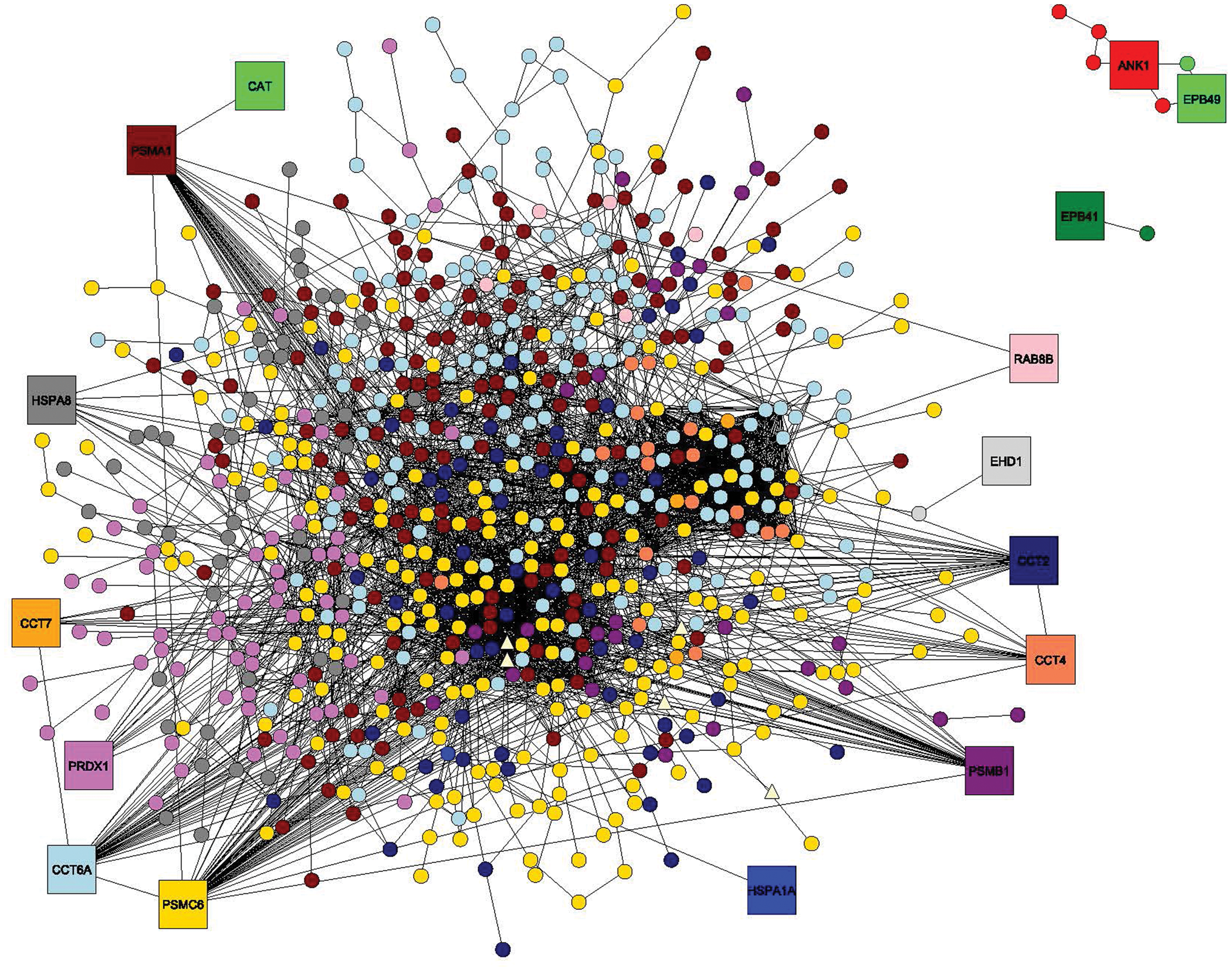

D’Alessandro et al. published a review summarizing the contemporary state of the RBC proteome and interactome as of 2010.¹² They merged the data from available RBC proteomics studies and performed pathway and network analysis using Ingenuity Software. Each gene identifier from the list they compiled was mapped to the corresponding gene object in the Ingenuity Pathway Knowledge Base. Of the 2086 proteins that were in the list originally, 1574 of those had a match in the database and were eligible for the network analysis, whereas 1374 proteins were eligible for pathway analysis. The association between the data set canonical and toxicity pathways was assigned a score, where the highest scores are proportional to a lower probability of casual association. The software identified 69 main canonical pathways and 850 different subpathways. When it comes to the network analysis, they focused on the top 50 subnetworks generated by the software. An in-depth examination showed that the top two ultra-networks share similar functions and at least one node. They concluded that ultra-networks display a well-ordered structure and are focused around the activity of several key nodes, in spite of the fact that some of them have as many as a few hundred nodes. They also considered the ROD box proposed by Goodman et al.¹ in their network and found that the results they obtained were in agreement with our analysis.^1,12

Future directions

What lies ahead of us in the field of erythrocyte, and SS, proteomics and interactomics. Five years from now, we believe that we will have seen the following advances.

It is reasonable to expect that improvements to mass spectrometers will allow us to better study those proteins that are present in extremely low copy number (1 to 100 copies). This will expand the known erythrocyte proteome. While it will not approach the number of unique proteins in nucleated cells, with a complete complement of organelles, there is no reason to believe that it will not be higher than today. If the sensitivity of our protein profiling approaches improves in parallel, then we will be able to ascertain the role of these low copy number proteins to erythrocyte-based disorders.

The further development of single cell proteomic technology^84–86 could allow the first comparison of the proteomes between individual ISCs versus RSCs from an SCD patient’s blood sample; comparisons of individual WBC classes’ proteomes in severe versus mild SCD and the effect of drug therapy on individual cells. While this statement concerns SCD, it should be apparent to the reader that the same will be true for any erythrocyte disorder or changes as blood bank blood ages or during normal or pathologic in vivo ageing of erythrocytes.

The fusion of proteomics with computational analysis and informatics has led to software which can couple interactome networks to the three-dimensional structure of the interacting proteins.^87–93 When this is coupled to software that can analyse the affinities and on/off rates of PPI, then we will have more valuable 3D interactome networks which will be able to accurately predict in silico the physiological effects of disease-related protein defects and the results of pharmaco-proteomic changes upon cellular homoeostasis. Five years from now, the combined software capabilities and MS hardware sophistication should be in place to link modified structure and function of proteins in SS erythrocytes and leukocytes to changes in their 3D interactome network that leads to the pathophysiology of SCD including the cellular interactions that lead to vasoocclusion.

Footnotes

Authors contributions

SRG wrote the proteomics and sickle cell sections. OD and MZ wrote the interactomics section and DGK did the research to develop Supplementary Table 1.

Acknowledgements

This work was supported by NSF grant CCF-0635013 to Ovidiu Daescu and the SD fund from SUNY Upstate for Steven R. Goodman.

References

Goodman

Kurdia

Ammann

Kakhniashvili

Daescu

. The human red blood cell proteome and interactome. Exp Biol Med 2007; 232(11): 1391–408.

Low

Seow

Chung

MCM

. Separation of human erythrocyte membrane associated proteins with one-dimensional and two-dimensional gel electrophoresis followed by identification with matrix-assisted laser desorption/ionization-time of flight mass spectrometry. Proteomics 2002; 2(9): 1229–39.

Kakhniashvili

Bulla

Jr Goodman

. The human erythrocyte proteome: Analysis by ion trap mass spectrometry. Mol Cell Proteomics 2004; 3(5): 501–9.

Tyan

Jong

Liao

. Proteomic profiling of erythrocyte proteins by proteolytic digestion chip and identification using two-dimensional electrospray ionization tandem mass spectrometry. J Proteome Res 2005; 4(3): 748–57.

Pasini

Kirkegaard

Mortensen

Lutz

Thomas

Mann

. In-depth analysis of the membrane and cytosolic proteome of red blood cells. Blood 2006; 108(3): 791–801.

Boschetti

Righetti

. Hexapeptide combinatorial ligand libraries: The march for the detection of the low-abundance proteome continues. BioTechniques 2008; 44(5): 663–5.

Alexandre

. Proteomic mining of the red blood cell: Focus on the membrane proteome. Expert Rev Proteomics 2010; 7(2): 165–8.

Lion

Tissot

. Application of proteomics to hematology: The revolution is starting. Expert Rev Proteomics 2008; 5(3): 375–9.

Liumbruno

D'Amici

Grazzini

Zolla

. Transfusion medicine in the era of proteomics. J Proteomics 2008; 71(1): 34–45.

10.

Zolla

. Proteomics and transfusion medicine. Blood Transfus 2008; 6(2): 67–9.

11.

Boschetti

Righetti

. The art of observing rare protein species in proteomes with peptide ligand libraries. Proteomics 2009; 9(6): 1492–510.

12.

D'Alessandro

Righetti

Zolla

. The red blood cell proteome and interactome: An update. J Proteome Res 2010; 9(1): 144–63.

13.

Liumbruno

D'Alessandro

Grazzini

Zolla

. How has proteomics informed transfusion biology so far? Crit Rev Oncol 2010; 76(3): 153–72.

14.

Liumbruno

D'Alessandro

Grazzini

Zolla

. Blood-related proteomics. J Proteomics 2010; 73(3): 483–507.

15.

Pasini

Lutz

Mann

Thomas

. Red blood cell (RBC) membrane proteomics – Part I: Proteomics and RBC physiology. J Proteomics 2010; 73(3): 403–20.

16.

Pasini

Lutz

Mann

Thomas

. Red blood cell (RBC) membrane proteomics – Part II: Comparative proteomics and RBC patho-physiology. J Proteomics 2010; 73(3): 421–35.

17.

Neelam

Kakhniashvili

Wilkens

Levene

Goodman

. Functional 20S proteasomes in mature human red blood cells. Exp Biol Med 2011; 236(5): 580–91.

18.

Bachi

Simó

Restuccia

. Performance of combinatorial peptide libraries in capturing the low-abundance proteome of red blood cells. 2. Behavior of resins containing individual amino acids. Anal Chem 2008; 80(10): 3557–65.

19.

Boschetti

Righetti

. The ProteoMiner in the proteomic arena: A non-depleting tool for discovering low-abundance species. J Proteomics 2008; 71(3): 255–64.

20.

Roux-Dalvai

de Peredo

Simó

. Extensive analysis of the cytoplasmic proteome of human erythrocytes using the peptide ligand library technology and advanced mass spectrometry. Mol Cell Proteomics 2008; 7(11): 2254–69.

21.

Simó

Bachi

Cattaneo

. Performance of combinatorial peptide libraries in capturing the low-abundance proteome of red blood cells. 1. Behavior of mono- to hexapeptides. Anal Chem 2008; 80(10): 3547–56.

22.

Bosman

GJCGM

Lasonder

Luten

. The proteome of red cell membranes and vesicles during storage in blood bank conditions. Transfusion 2008; 48(5): 827–35.

23.

Bosman

GJCGM

Lasonder

Groenen-Döpp

YAM

Willekens

FLA

Werre

Novotný

VMJ

. Comparative proteomics of erythrocyte aging in vivo and in vitro. J Proteomics 2010; 73(3): 396–402.

24.

D'Amici

Rinalducci

Zolla

. Proteomic analysis of RBC membrane protein degradation during blood storage. J Proteome Res 2007; 6(8): 3242–55.

25.

Helbig

Heck

AJR

Slijper

. Exploring the membrane proteome-challenges and analytical strategies. J Proteomics 2010; 73(5): 868–78.

26.

van Gestel

van Solinge

van der Toorn

HWP

. Quantitative erythrocyte membrane proteome analysis with blue-Native/SDS PAGE. J Proteomics 2010; 73(3): 456–65.

27.

Wang

Chen

Liu

Zhao

. Four-dimensional orthogonal electrophoresis system for screening protein complexes and protein–protein interactions combined with mass spectrometry. J Proteome Res 2010; 9(10): 5325–34.

28.

De Palma

Roveri

Zaccarin

. Extraction methods of red blood cell membrane proteins for multidimensional protein identification technology (MudPIT) analysis. J Chromatogr A 2010; 1217(33): 5328–36.

29.

Pesciotta

Sriswasdi

Tang

Mason

Bessler

Speicher

. A label-free proteome analysis strategy for identifying quantitative changes in erythrocyte membranes induced by red cell disorders. J Proteomics 2012; 76(5): 194–202.

30.

Florens

Liu

Wang

. Proteomics approach reveals novel proteins on the surface of malaria-infected erythrocytes. Mol Biochem Parasitol 2004; 135(1): 1–11.

31.

Fontaine

Bourdon

Belghazi

. Plasmodium falciparum infection-induced changes in erythrocyte membrane proteins. Parasitol Res 2012; 110(2): 545–56.

32.

Kuss

Gan

Gunalan

Bozdech

Sze

Preiser

. Quantitative proteomics reveals new insights into erythrocyte invasion by Plasmodium falciparum. Mol Cell Proteomics 2012; 11(2): 1–14.

33.

Lasonder

Treeck

Alam

Tobin

. Insights into the Plasmodium falciparum schizont phospho-proteome. Microb Infect 2012; 14(10): 811–9.

34.

Méndez

Hernáez

Kamali

Diez

Puyet

Bautista

. Differential carbonylation of cytoskeletal proteins in blood group O erythrocytes: Potential role in protection against severe malaria. Infect Genet Evol 2012; 12(8): 1780–7.

35.

Millholland

Chandramohanadas

Pizzarro

. The malaria parasite progressively dismantles the host erythrocyte cytoskeleton for efficient egress. Mol Cell Proteomics 2011; 10(12): 1–12.

36.

Nelson

Quaile

Xia

Wastling

Craig

. Identification of phosphorylated proteins in erythrocytes infected by the human malaria parasite Plasmodium falciparum. Malaria J 2009; 8(1): 105–105.

37.

Demiralp

Peker

Turgut

Akar

. Comprehensive identification of erythrocyte membrane protein deficiency by 2D gel electrophoresis based proteomic analysis in hereditary elliptocytosis and spherocytosis. Proteomics – Clin Appl 2012; 6(7–8): 403–11.

38.

Peker

Akar

Demiralp

. Proteomic identification of erythrocyte membrane protein deficiency in hereditary spherocytosis. Mol Biol Rep 2012; 39(3): 3161–7.

39.

Saha

Ramanathan

Basu

Banerjee

Chakrabarti

. Elevated levels of redox regulators, membrane-bound globin chains, and cytoskeletal protein fragments in hereditary spherocytosis erythrocyte proteome. Eur J Haematol 2011; 87(3): 259–66.

40.

von Löhneysen

Scott

Soldau

Friedman

. Assessment of the red cell proteome of young patients with unexplained hemolytic anemia by two-dimensional differential in-gel electrophoresis (DIGE). PLoS ONE 2012; 7(4): e34237–e34237.

41.

Wilkinson

Turner

Parkin

. Membrane raft actin deficiency and altered Ca2+-induced vesiculation in stomatin-deficient overhydrated hereditary stomatocytosis. Biochim Biophys Acta – Biomembr 2008; 1778(1): 125–32.

42.

Bhattacharya

Saha

Basu

. Differential regulation of redox proteins and chaperones in HbEβ-thalassemia erythrocyte proteome. Proteomics – Clin Appl 2010; 4(5): 480–8.

43.

Chakrabarti

Bhattacharya

Basu

Saha

Halder

. Differential expression of red cell proteins in hemoglobinopathy. Proteomics – Clin Appl 2011; 5(1–2): 98–108.

44.

Blasi

D'Alessandro

Ramundo

Zolla

. Red blood cell storage and cell morphology. Transfus Med 2012; 22(2): 90–6.

45.

Bosman

GJCGM

Lasonder

Groenen-Döpp

YAM

Willekens

FLA

Werre

. The proteome of erythrocyte-derived microparticles from plasma: New clues for erythrocyte aging and vesiculation. J Proteomics 2012; 76: 203–10.

46.

Cluitmans

JCA

Hardeman

Dinkla

Brock

Bosman

GJCGM

. Red blood cell deformability during storage: Towards functional proteomics and metabolomics in the blood bank. Blood Transfus 2012; 10(Suppl. 2): s8–14.

47.

Dinkla

Novotný

VMJ

Joosten

Bosman

GJCGM

. Storage-induced changes in erythrocyte membrane proteins promote recognition by autoantibodies. PLoS ONE 2012; 7(8): e42250–e42250.

48.

Mohanty

Shukla

Williamson

Launer

Saxena

Rifkind

. Alterations in the red blood cell membrane proteome in Alzheimer's subjects reflect disease-related changes and provide insight into altered cell morphology. Proteome Sci 2010; 8: 11–11.

49.

Huang

Wang

Prabakaran

. Independent protein-profiling studies show a decrease in apolipoprotein A1 levels in schizophrenia CSF, brain and peripheral tissues. Mol Psychiatr 2008; 13(12): 1118–28.

50.

Prabakaran

Wengenroth

Lockstone

Lilley

Leweke

Bahn

. 2-D DIGE analysis of liver and red blood cells provides further evidence for oxidative stress in schizophrenia. J Proteome Res 2007; 6(1): 141–9.

51.

Sun

Jia

Fanous

. Schizophrenia gene networks and pathways and their applications for novel candidate gene selection. PLoS ONE 2010; 5(6): e11351–e11351.

52.

Alexandre

Charro

Blonder

. Profiling the erythrocyte membrane proteome isolated from patients diagnosed with chronic obstructive pulmonary disease. J Proteomics 2012; 76: 259–269.

53.

Alvarez-Llamas

Zubiri

Maroto

. A role for the membrane proteome in human chronic kidney disease erythrocytes. Translat Res 2012; 160(5): 374–83.

54.

Jiang

Jia

Jiang

. Protein dysregulation in red blood cell membranes of type 2 diabetic patients. Biochem Biophys Res Commun 2003; 309(1): 196–200.

55.

Zhang

Monroe

Schepmoes

. Comprehensive identification of glycated peptides and their glycation motifs in plasma and erythrocytes of control and diabetic subjects. J Proteome Res 2011; 10(7): 3076–88.

56.

Yuditskaya

Suffredini

Kato

. The proteome of sickle cell disease: Insights from exploratory proteomic profiling. Expert Rev Proteomics 2010; 7(6): 833–48.

57.

Shartava

Monteiro

Aladar Bencsath

. A posttranslational modification of β-actin contributes to the slow dissociation of the spectrin-protein 4.1-actin complex of irreversibly sickled cells. J Cell Biol 1995; 128(5): 805–18.

58.

Shartava

Miranda

Williams

Shah

Monteiro

Goodman

. High density sickle cell erythrocyte core membrane skeletons demonstrate slow temperature dependent dissociation. Am J Hematol 1996; 51(3): 214–9.

59.

Shartava

Korn

Shah

Goodman

. Irreversibly sickled cell β-actin: Defective filament formation. Am J Hematol 1997; 55(2): 97–103.

60.

Bencsath

Shartava

Monteiro

Goodman

. Identification of the disulfide-linked peptide in irreversibly sickled cell β-actin. Biochemistry (New York) 1996; 35(14): 4403–8.

61.

Monteiro

Gibson

Shartava

Goodman

. Preliminary characterization of a structural defect in homozygous sickled cell alpha spectrin demonstrated by a rabbit autoantibody. Am J Hematol 1998; 58(3): 200–5.

62.

Ghatpande

Goodman

. Ubiquitination of spectrin regulates the erythrocyte spectrin-protein-4.1-actin ternary complex dissociation: Implications for the sickle cell membrane skeleton. Cell Mol Biol (Noisy-le-grand) 2004; 50(1): 67–74.

63.

Mishra

Goodman

. Ubiquitination of erythrocyte spectrin regulates the dissociation of the spectrin-adducin-f-actin ternary complex in vitro. Cell Mol Biol (Noisy-le-grand) 2004; 50(1): 75–80.

64.

Riahi

Kakhniashvili

Goodman

. Ubiquitination of red blood cell α-spectrin does not affect heterodimer formation. Am J Hematol 2005; 78(4): 281–7.

65.

Chang

Kakhniashvili

Goodman

. Spectrin’s E2/E3 ubiquitin conjugating/ligating activity is diminished in sickle cells. Am J Hematol 2005; 79(2): 89–96.

66.

Kakhniashvili

Chaudhary

Zimmer

Aladar Bencsath

Jardine

Goodman

. Erythrocyte spectrin is an E2 ubiquitin conjugating enzyme. Biochemistry (New York) 2001; 40(38): 11630–42.

67.

Chang

Cubillos

Kakhniashvili

Goodman

. Ankyrin is a target of spectrin's E2/E3 ubiquitin-conjugating/ligating activity. Cell Mol Biol (Noisy-le-grand) 2004; 50(1): 59–66.

68.

Chang

Cubillosi

Kakhniashvili

Goodman

. Band 3 is a target protein of spectrin's E2/E3 activity: Implication for sickle cell disease and normal red blood cell aging. Cell Mol Biol (Noisy-le-grand) 2004; 50(2): 171–7.

69.

Hsu

Zimmer

Goodman

. Erythrocyte spectrin's chimeric E2/E3 ubiquitin conjugating/ligating activity. Cell Mol Biol 2005; 51(2): 187–93.

70.

Hsu

Goodman

. Spectrin and ubiquitination: A review. Cell Mol Biol (Noisy-le-grand) 2005, (Suppl 51OL801–807.

71.

Goodman

. The irreversibly sickled cell: A perspective. Cell Mol Biol (Noisy-le-grand) 2004; 50(1): 53–8.

72.

Gibson

Shartava

McIntyre

. The efficacy of reducing agents or antioxidants in blocking the formation of dense cells and irreversibly sickled cells in vitro. Blood 1998; 91(11): 4373–8.

73.

Pace

Shartava

Pack-Mabien

Mulekar

Ardia

Goodman

. Effects of N-acetylcysteine on dense cell formation in sickle cell disease. Am J Hematol 2003; 73(1): 26–36.

74.

Kakhniashvili

Griko

Bulla Jr . LA, Goodman SR. The proteomics of sickle cell disease: Profiling of erythrocyte membrane proteins by 2D‐DIGE and tandem mass spectrometry. Exp Biol Med 2005; 230(11): 787–92.

75.

Chou

Choudhary

Goodman

. Protein profiling of sickle cell versus control rbc core membrane skeletons by icat technology and tandem mass spectrometry. Cell Mol Biol Lett 2006; 11(3): 326–37.

76.

Hryniewicz-Jankowska

Choudhary

Goodman

. Variation in the monocyte proteome. Exp Biol Med 2007; 232(7): 967–76.

77.

Hryniewicz-Jankowska

Choudhary

Ammann

Quinn

Goodman

. Monocyte protein signatures of disease severity in sickle cell anemia. Exp Biol Med 2009; 234(2): 210–21.

78.

Ghatpande

Choudhary

Quinn

Goodman

. Pharmaco-proteomic study of hydroxyurea-induced modifications in the sickle red blood cell membrane proteome. Exp Biol Med 2008; 233(12): 1510–7.

79.

Ghatpande

Choudhary

Quinn

Goodman

. In vivo pharmaco-proteomic analysis of hydroxyurea induced changes in the sickle red blood cell membrane proteome. J Proteomics 2010; 73(3): 619–26.

80.

Kurdia A, Daescu O, Ammann L, Kakhniashvili D, Goodman SR. Centrality measures for the human red blood cell interactome. Engineering in Medicine and Biology Workshop, IEEE Dallas, 2007:98–101.

81.

Ammann

Goodman

. Cluster analysis for the impact of sickle cell disease on the human erythrocyte protein interactome. Exp Biol Med 2009; 234(6): 703–11.

82.

Zivanic

Daescu

Kurdia

Goodman

. The Voronoi diagram for graphs and its application in the sickle cell disease research. J Comput Sci 2012; 3(5): 335–43.

83.

Erwig

. Graph Voronoi diagram with applications. Networks 2000; 36(3): 156–63.

84.

Bendall

Nolan

. From single cells to deep phenotypes in cancer. Nat Biotechnol 2012; 30(7): 639–47.

85.

Bodenmiller

Zunder

Finck

. Multiplexed mass cytometry profiling of cellular states perturbed by small-molecule regulators. Nat Biotechnol 2012; 30(9): 858–67.

86.

Schulz

Danna

Krutzik

Nolan

. Single-cell phospho-protein analysis by flow cytometry. Curr Protoc Immunol 2012; (Suppl. 96): 8.17.1–8.17.20.

87.

de Vries

Bonvin

AMJJ

. Cport: A consensus interface predictor and its performance in prediction-driven docking with HADDOCK. PLoS ONE 2011; 6(3): e17695–e17695.

88.

Hennig

de Vries

Hennig

KDM

. MTMDAT-HADDOCK: High-throughput, protein complex structure modeling based on limited proteolysis and mass spectrometry. BMC Struct Biol 2012; 29.

89.

Karaca

Bonvin

AMJJ

. A multidomain flexible docking approach to deal with large conformational changes in the modeling of biomolecular complexes. Structure 2011; 19(4): 555–65.

90.

Melquiond

Karaca

Kastritis

Bonvin

. Next challenges in protein-protein docking: From proteome to interactome and beyond. Wiley Interdis Rev: Comput Mol Sci 2012; 2(4): 642–51.

91.

Rodrigues

JPGLM

Trellet

Schmitz

. Clustering biomolecular complexes by residue contacts similarity. Proteins: Struct Funct Bioinformatics 2012; 80(7): 1810–7.

92.

Stein

Aloy

. Novel peptide-mediated interactions derived from high-resolution 3-dimensional structures. PLoS Comput Biol 2010; 6(5): 1–16.

93.

Wang

Wei

Thijssen

Das

Lipkin

. Three-dimensional reconstruction of protein networks provides insight into human genetic disease. Nat Biotechnol 2012; 30(2): 159–64.

94.

yEd Graph Editor. See http://www.yworks.com/en/products_yed_about.html.

Supplementary Material

Please find the following supplemental material available below.

For Open Access articles published under a Creative Commons License, all supplemental material carries the same license as the article it is associated with.

For non-Open Access articles published, all supplemental material carries a non-exclusive license, and permission requests for re-use of supplemental material or any part of supplemental material shall be sent directly to the copyright owner as specified in the copyright notice associated with the article.

0.00 MB

0.10 MB