k -degree coverage algorithm based on optimization nodes deployment in wireless sensor networks

Abstract

In the process of the wireless sensor network research, the issue on the energy consumption and coverage is an essential and critical one. According to the characteristic of the sensor nodes, it is homogeneous, and we proposed the k-degree coverage algorithm based on optimization nodes deployment. First, the algorithm gives the solving procedure of the maximum seamless coverage ratio, when the three-node joint coverage has been provided. Second, when the sensor nodes are covering the monitoring area, the algorithm gives the solving procedure of the expected coverage quality and the judgment methods of the coverage ratio, when the nodes are compared with the nearby ones. And when there is redundancy coverage in the given monitoring area, we have given the solving procedure of any sensor nodes that exist in the redundant nodes coverage. Finally, using the simulation experiment, the results of the coverage algorithm based on optimization nodes deployment are compared with other algorithms in terms of the coverage quality and the network lifetime, the performance indexes have enhanced to 13.36% and 12.92% on average. Thus, the effectiveness and viability of the coverage algorithm based on optimization nodes deployment have been proved.

Keywords

Wireless sensor networks sensor nodes networks lifetime coverage ratio optimization deployment

Introduction

The wireless sensor network is a new type of network system, which is connected by thousands of sensors in the way of self-organizing and hybrid-hop; it is also the organic unification of the world of information and the physical world, which has realized the operation of the acquisition, computation, communication, and storage of the data.^1–3 With the rapid development of information technology, the wireless sensor network can be mainly applied in all kinds of engineering fields, such as the military affair, environment monitoring, disaster relief, smart home, health care, agricultural production, and transportation.^4–7

The energy consuming and the coverage quality of the network are the two key points in the field of wireless sensor network research.^8–10 The coverage quality will affect the monitoring effectiveness on moving target; its behavior characteristic is mainly reflected in the deployment mode of sensor node. The energy consumption of the network is shown as the effective reduction of the sensor nodes’ quick energy consumption, which can prolong the lifetime of the whole network. The coverage quality and the rapid energy consumption mainly depend on the rationality of sensor nodes deployment.^11,12 Generally, because of the limitation of the topographic, geomorphic conditions, and the environmental factors, we usually take the methods of the stochastic deployment to handle with the deployment of the sensor nodes. Due to its randomness, in the process of the deployment, the specific location of the sensor nodes cannot be predicted, so there are several or plenty of sensor nodes in a certain monitoring area or point, which can form the k-degree coverage finally. In the process of the stochastic deployment, it is possible that there are no sensor nodes covering at all in a certain monitoring area or point, which can form coverage holes. Thus, the effective coverage can be achieved by adding sensor nodes. Both of the cases can achieve the expected coverage effectiveness, but both have their own disadvantages.^13,14 First, plenty of sensor nodes gather in high density, generating lots of redundant information, which will cause congestion in the communication linkage, suppress the expandability of the network, lower the service quality of the network, and shorten the whole lifetime of the network.¹⁵ Second, when the concerned targets are in the coverage hole, we cannot take the real-time monitoring and coverage of the goal nodes. For sensor nodes, if they cannot provide accurate data information to sink nodes, there will be deviations and uncertainties in the data information that sink nodes have collected. Third, several work periods later, the sensor nodes will present the characteristic of heterogeneous sensor nodes. Because of the heterogeneous, it makes the whole sensor coverage area to change. Once the goal nodes shifted their statuses from covered to not covered, all the collected data information of goal nodes would lose their meanings. Fourth, the essentiality of the coverage is not the complete coverage of all the goal nodes, but the effective coverage of the concerned goal nodes. The essentiality of effective coverage is that when the concerned moving goal nodes are passing through the monitoring areas, the sensor nodes will complete their coverage first; simultaneously they will wake up their joint nodes to complete the linkage coverage, and then the collected data information will be uploaded to sink nodes.

Materials and methods

In the wireless sensor network research field, the issue of the network energy consumption and the effective coverage is a key one and an essential one that supports other special indexes of the wireless sensor network. Recent years, many experts, scholars at home and abroad have carried out plenty of researches thoroughly and carefully. Adulyasas et al.¹⁶ take the symmetry of the regular hexagon of a given circle as the research object and propose the connected coverage optimization algorithm, which can reduce the overlapping coverage area to improve the effective coverage of the whole monitoring area. Sun et al.¹⁷ propose the enhanced coverage control algorithm. When the monitoring area is covered, the algorithm gives the solving procedure of the expected value of the coverage quality. It also tests the proportion function relationship among various parameters, when the random variables are independent of each other. Besides, it also completes the effective coverage of the whole monitoring area by adjusting the adjustable parameter. Satisfying the presupposition of the network connection, Liao et al.¹⁸ complete the coverage of goal nodes by taking advantages of the moving characteristic of the sensor nodes. Thus, it proposes the heuristic algorithm, taking the Thiessen polygon as the active area to reduce the sensor nodes’ energy consumption to balance the network energy, proposing the sensor network coverage.

Sun et al.¹⁹ propose the maximum lifetime of reinforced barrier-coverage algorithm. The algorithm starts from the moving goal nodes going through the monitoring area. It takes advantages of the associate attribute of the sensor nodes and their neighbor nodes to complete the continuous coverage of the moving goal nodes. Finally, it achieves the complete coverage of the goal nodes. Sahoo and Sheu²⁰ propose the distributed connectivity and coverage maintenance algorithm (CoCo). The algorithm keeps the connection of the whole network by the work nodes awakening the redundant nodes. The restricted movement of sensor nodes ensures the goal nodes’ effective coverage, which limits the energy consumption caused by the monitoring distance to extend the lifetime of network. Meng et al.²¹ propose the scheduling control algorithm (SCA) based on the awareness model. The algorithm builds the awareness model taking advantages of the connection of the network and the nodes; it computes and chooses the minimum work nodes to guarantee the maximum coverage quality by the performance parameter relationship of the monitoring area of the nodes. Mini et al.²² bring in the artificial intelligence algorithms, the swarm intelligence algorithm, and the granule algorithm to complete the nodes deployment of the whole network monitoring area; in the stage of coverage optimization, the whole coverage is optimized by the two artificial intelligence algorithms and finally realizes the complete coverage of the monitoring area; as for the energy consumption, it completes the scheduling conversion of the node energy by the heuristic node scheduling, which extends the lifetime of the network. While Li et al.²³ bring in the partial parameter α, utilize the partial coverage optimization, constitute the partial αcoverage, after a series of calculation and optimization of the α, the complete coverage optimization is finally achieved. All the above-mentioned algorithms have achieved the effective coverage of the monitoring area to some extent; however, they have the mutual problem that the algorithms have more calculations, they are more complex, and the scalability of the wireless sensor network is worse.

Zhao et al.²⁴ propose the optimization strategy on coverage algorithm based on Voronoi. Having satisfied the condition of a certain coverage quality, the algorithm can add some work nodes to coverage holes to improve the current coverage ratio. Meanwhile, it will search reasonable information of repairing site to guarantee the connection of the whole network. Hanid et al.²⁵ also take the Voronoi as the research objective, solve the information of wire rod site that is formed by the geometry variation in the Voronoi of the sensor nodes, and finally, it completes the coverage of the monitoring area. Sahoo and Sheu²⁰ and Yuchee et al.²⁶ calculate the goal nodes effectively, utilizing different angles of the sector that composed by the sensor nodes and the goal nodes. They also give the method of computing the coverage ratio of different monitoring areas. All the above-mentioned algorithms have the better feasibility and the higher reliability, but the network models and the algorithms are too complex when they are put into research.

From Zhao et al.,²⁴ Hanid et al.,²⁵ and Yuchee et al.,²⁶ they all take the static goal nodes as the research objective, Wang et al.²⁷ do not consider the situation when the moving targets are the concerned goal nodes, what the k-barrier coverage will be. Xing et al.²⁸ propose the polytypic target coverage algorithm based on the linear programming. The algorithm utilizes the clustering structure to solve the polytypic target coverage problem. By computing the coverage ability and the residual energy of the sensor, it completes the polytypic target optimization coverage in the way of the linear programming. Sun et al.²⁹ propose the event probability driven mechanism (EPDM). First, EPDM algorithm builds the network model that is covered by the sensor nodes and the goal nodes, then it calculates the coverage ratio of the sensor nodes and the goal nodes with the help of the probability, and finally, it will complete the changing states among the nodes by the node-scheduling algorithm, which achieves the purpose of extending the lifetime of the network. Under certain conditions, all the above-mentioned algorithms can complete the effective coverage of the goal nodes in the monitoring area to extend the lifetime of the network.

With the aid of the basic ideas in Xing et al.²⁸ and Sun et al.,²⁹ the coverage algorithm based on optimization nodes deployment (CAOND) algorithm gives the solving procedure of the maximum coverage area when there is three-node joint; it verifies the expected value of the coverage quality of the goal nodes in the monitoring area by utilizing some related theoretical knowledge of the probabilistic theory. Meanwhile, it compares the proportionate relationship of the awareness intensity of the joint nodes and the single nodes; it also gives the coverage judgment method of any sensor nodes in the redundancy nodes. Finally, we took the simulation experiment to testify the CAOND algorithm. The result showing that both the coverage ratio and the lifetime of the network have improved a lot, which has verified the effectiveness and the feasibility of the algorithm in this article.

For the deficiencies and shortcomings of the research, the main contributions of this article will be presented in the following five points:

Having studied and analyzed some relevant literature information at home and abroad, with the help of the theoretical idea from the literature, we proposed the CAOND algorithm.

Through the relevant geometry and the three-node joint, the article gives the derivation procedure of the maximum seamless joint coverage ratio. Besides, it also calculates the maximum effective coverage ratio, when the three-node joint coverage has been completed.

In the monitoring area, k nodes are selected at random to be the object of study. Based on the probability theory taking advantages of the characteristic of sensor nodes’ sending range, the solving procedure of the expected value is given, when there are k nodes covering jointly.

When the goal nodes are covered by joint network nodes or single nodes, the comparative methods of the awareness intensity are given. By limiting the value range of the adjustable parameter λ, we also provide the judgment method of redundancy coverage of any sensor nodes being covered by redundant nodes.

Through the simulation experiment, compared with other algorithm, we verify the effectiveness and feasibility of the CAOND algorithm.

Prerequisite knowledge

Table 1 illustrates the symbols used in this article.

Table 1.

Parameter description.

Parameter	Description	Parameter	Description
S	The monitored area	R ₀	The expectation value of sensor radium
S_i	The sensor node for i	σ ²	Variance
N	The number of sensor nodes	d	Euclidean distance between nodes
R	The sensing radium	W	Sensing strength of nodes

All the sensor nodes are deployed at a two-dimensional (2D) monitoring area at random; they have the following characteristics:

At the initial time, all the perceived radii of the sensor nodes are the same, and it equals to the energy.

All the perceived radii of the sensor nodes comply with the normal distribution; it is much less than the length of the monitoring area and ignores the boundary effect.

The communication range is equal or greater than the two times the value of the perceived radius.

All the sensor nodes are independent of each other and are equal to each other.

Definition 1 (k-barrier coverage)

A certain goal node is covered by k sensor nodes at least, and it is called as the k-barrier coverage.

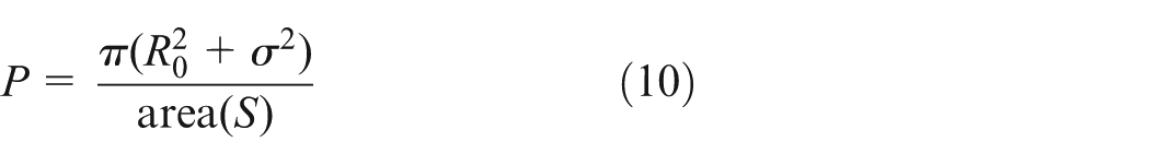
Definition 2 (network coverage probability)

In the monitoring area, the specific value of the effective coverage area and the monitoring area is called as the network coverage rate. The physical significance of the network coverage rate is that the bigger the coverage rate is, the better the coverage quality is

p = \frac{area ((⋃_{i = 1, 2, \dots, N} s_{i}) ⋂ area (S))}{area (S)}

(1)

In the formula, the area(S) symbolizes the monitoring area, the $⋃_{i = 1, 2 \dots N} s_{i}$ is the sum of the coverage areas of the sensor nodes, and s_i symbolizes the ith sensor node.

Definition 3 (effective coverage probability)

It is the specific value of the effective area of the sensor nodes with the area of the sensor nodes in the monitoring area. The effective area of the sensor nodes is the area, which is covered by several times but only need calculated once, when several sensor nodes are completing the k-coverage. Definition 2 provided the network coverage probability, which is the specific value of the effective area of the sensor nodes with the area of the monitoring area

P_{e} = \frac{area ((⋃_{i = 1, 2, \dots, N} s_{i}) ⋂ area (S))}{area (⋃_{i = 1, 2, \dots, N} s_{i})}

(2)

Theorem 1

When the three nodes are seamlessly integrated jointly, the maximum coverage area can be shown as $S_{max} = ((4 π + 3 \sqrt{3}) r^{2}) / 2$ ; the maximum effective coverage rate is 94.24%. r symbolizes the perceived radius of the sensor nodes and s symbolizes the maximum coverage area.

Proof

As shown in Figure 1, supposing that the shaded area is S₁, the area of the sector OACB is S₂ and the area of the regular triangle is S₃. Because the coverage area should be the maximum one, the three sensor nodes will meet at the point B; from the symmetry and the concentric circles of the same string theorem, the center chord of the shaded area is one of the sides of the regular hexagon of the given Circle O, that is to say the sector OACB is one-sixth of the Circle O, the central angle of the string is π/3, so the ΔOAB is the regular triangle, OA = AB = BO = r

S_{1} = 2 (S_{2} - S_{3}) = \frac{(2 π - 3 \sqrt{3}) r^{2}}{6}

(3)

S_{max} = 3 (π r^{2} - S_{1}) = 3 (\frac{4 π r^{2} - 3 \sqrt{3} r^{2}}{6}) = \frac{(4 π + 3 \sqrt{3}) r^{2}}{2}

(4)

Figure 1.

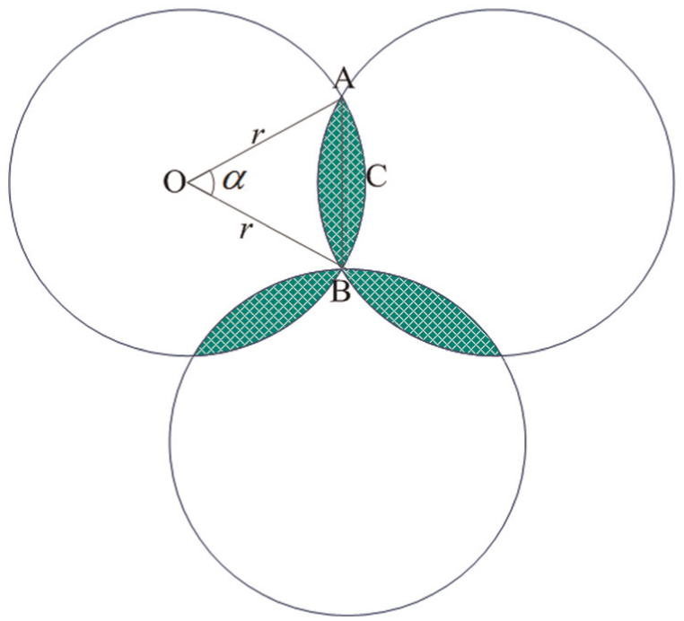
The three-node seamless joint diagrammatic sketch.

So the maximum effective coverage rate is as follows

P_{e} = \frac{S_{m a x}}{3 π r^{2}} = \frac{4 π + 3 \sqrt{3}}{6 π} = 94.24 %

(5)

Analysis of the coverage quality

Basic idea

To solve the issue of the redundant sensor nodes, the redundant connected graph of sensor nodes should be built first. It means that all the sensor nodes can calculate the redundant information with their neighbor nodes by a certain location algorithm, such as the centroid location and the received signal strength indicator (RSSI) range-based localization; they fuse themselves in their own cluster and then send the result to the sink nodes through the communication linkage.³⁰ When the sink nodes receive the redundant information, after calculating and analyzing the information, the redundant relationship connected graph G can be built according to the results. The degree of the connected graph is the number of the relevant limited information corresponding to the redundancy rate of the sensor nodes. When the number of the sensor nodes is adding, the redundancy rate is upping. In the connected graph G, when the redundancy rate is more than the threshold that is set in advance, the state of the node will turn to sleep. At the same time, when there are n (n > 2) high-redundant nodes in the connectivity graph G, taking the energy as the choice condition, the highest energy nodes are selected as the sleeping nodes taking advantages of ranking algorithm. Meanwhile, the nodes and their neighbors will be deleted, then iterate them by the iterative method to find the next high-energy nodes until the redundant rates of all the sensor nodes in the connected graph A are less than the threshold. In the energy consumption, the article manages the managing node and the member node with the help of clustering principle. At the first stage of the network, member node sends a piece of information, inf_coverag to sink node, the information inf_coverag including the location information, the ID information, and the energy information. After one round or several rounds, the sink nodes receive the information from all the sensor nodes, calculate the information, and store the node-energy at the Store List CL. The nodes are sorted from highness to the lowliness according to the rest energy. The nodes at the frontier range have higher ability to cover. The managing node will find the sensor node that corresponds with the covering conditions among the List CL, according to the location information of the goal nodes. It will send information, inf_coverag to that sensor node to realize the effective coverage, the rest nodes are sleeping, which achieves the goal of saving network energy cost.

Expected value of coverage quality

In the above section, we give the solving method and the procedure of the proof of the maximum coverage area when the three nodes are jointed seamlessly. In the monitoring area, the sensor nodes need to complete the operations, such as the data acquisition, the data communication, the behavioral features of which can mainly be reflected in the distribution density of the sensor nodes throwing at random. The distribution density can affect the coverage quality directly; stable network does not only need the reasonable network service system, but also need a feasible coverage system.^31–33 To meet the prerequisite of a certain coverage rate, if the effective coverage of the monitoring area was completed, the expected coverage value of the monitoring area would be computed.

Theorem 2

In the monitoring area S, k nodes are chosen at random; their expected value needs to be completed

E (P) = 1 - {(1 - \frac{π (R_{0}^{2} + σ^{2})}{area (S)})}^{k}

Proof

Because sensor nodes thrown in the monitoring areas at random comply with the uniform distribution, the coverage rate P_a of any sensor nodes in the monitoring is as follows

P_{a} = \frac{π r^{2}}{area (S)}

(6)

Because the perceived radius of sensor nodes complies with the normal distribution (R₀, σ²), in the monitoring area, the coverage rate of any goal nodes covered by sensor nodes is as follows

P = \int_{0}^{2 R_{0}} P_{a} \frac{1}{\sqrt{2 π} σ} \exp (- \frac{{(r - R_{0})}^{2}}{2 σ^{2}}) d r

(7)

Making x = (r − R₀)/σ, so

P = {(\frac{π}{2})}^{\frac{1}{2}} \frac{1}{area (S)} \int_{R_{0} / σ}^{R_{0} / σ} {(x σ + R_{0})}^{2} \exp (- \frac{x^{2}}{2}) dx

(8)

Obtained by the calculation

\begin{matrix} P = {(\frac{π}{2})}^{\frac{1}{2}} \frac{1}{area (S)} (\int_{- R_{0} / σ}^{R_{0} / σ} σ^{2} x^{2} \exp (- \frac{x^{2}}{2}) d x + \int_{- R_{0} / σ}^{R_{0} / σ} 2 σ x \exp (- \frac{x^{2}}{2}) d x + \int_{- R_{0} / σ}^{R_{0} / σ} R_{0}^{2} \exp (- \frac{x^{2}}{2}) d x) \\ = {(\frac{π}{2})}^{\frac{1}{2}} \frac{1}{area (S)} (- σ^{2} x \exp (- \frac{x^{2}}{2}) |_{- \frac{R_{0}}{σ}}^{\frac{R_{0}}{σ}}) + {(\frac{π}{2})}^{\frac{1}{2}} (σ^{2} + R_{0}^{2}) \end{matrix}

(9)

On simplifying formula (9), we get

P = \frac{π (R_{0}^{2} + σ^{2})}{area (S)}

(10)

The sensor nodes districted in the monitoring area at random are independent of each other, so in the monitoring area, the expected coverage value of any goal nodes covered by the sensor nodes is as follows

E (P) = 1 - {(1 - \frac{π (R_{0}^{2} + σ^{2})}{area (S)})}^{k}

(11)

Corollary 1

To complete the effective coverage of the monitoring area, the minimum of the nodes is

\frac{\ln (1 - ((π r^{2}) / (area (S))))}{\ln (1 - ((π (R_{0}^{2} + σ^{2})) / (area (S))))}

Proof

Supposing that the minimum of the sensor nodes deployed in the monitoring area is n. According to Theorem 2, the expected value of the goal nodes covered by any sensor node is as follows

\frac{π r^{2}}{area (S)} \leq 1 - {(1 - \frac{π (R_{0}^{2} + σ^{2})}{area (S)})}^{n}

(12)

After taking the logarithm of the both sides of formula (12)

n \ln (1 - \frac{π (R_{0}^{2} + σ^{2})}{area (S)}) \leq \ln (1 - \frac{π r^{2}}{area (S)})

(13)

Seeking n

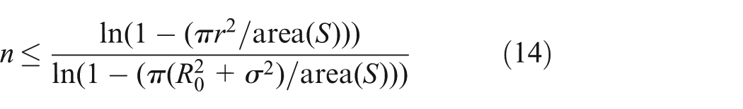
n \leq \frac{\ln (1 - (π r^{2} / area (S)))}{\ln (1 - (π (R_{0}^{2} + σ^{2}) / area (S)))}

(14)

Thus, to complete the effective coverage of the monitoring area, the required minimum of sensor nodes should be $(\ln (1 - ((π r^{2}) / (area (S))))) / (\ln (1 - ((π (R_{0}^{2} + σ^{2})) / (area (S)))))$ .

Nodes coverage probability

Definition 4 (neighbor node)

The distance between any two nodes s_i, s_j is less than the double times of the perceived radius that is called as the neighbor node

d = \sqrt{{(x_{i} - x_{j})}^{2} + {(y_{i} - y_{j})}^{2}} \leq 2 r

(15)

In formula (15), the (x_i,y_i) and the (x_j,y_j) are the coordinate values of the two sensor nodes s_i, s_j, the d is the Euclidean distance between the two sensor nodes, and the r is the perceived radius of the sensor nodes.

Definition 5 (awareness intensity)

The awareness intensity of any sensor node s at the point is α²⁵

I = {\begin{matrix} e^{- α d_{(s, a)}} 0 < d_{(s, a)} \leq r \\ 0 r < d_{(s, a)} \end{matrix}

(16)

In formula (16), the d_(s,a) is the Euclidean distance between the sensor node s and any point α, α is the physical parameter of the perceptive module, and r is the perceived radius of the sensor nodes. Supposing that the joint nodes set is T, so the awareness intensity of the joint nodes set at the point α is

I (T, a) = 1 - \underset{s_{i} \in T}{Π} (1 - I (s_{i}, a))

(17)

The expression form of formula (17) is quite similar to the probability expression form of at least one of the nodes that are covered by the n sensor nodes. Zairi et al.⁸ and Zhu et al.⁹ have provided the relevant proof. Thus, in the monitoring area, the awareness intensity of a certain point can be converted into the probability expression form of the certain point. Because of the sensor nodes’ randomness states deployed in the monitoring area, when the concerned moving goal nodes are covered by sensor nodes or single nodes, in order to know how to identify the awareness intensity of sensor nodes and single nodes to enhance effective coverage of the coverage area, we brought in Theorem 3.

Theorem 3

Within the unique sensing range, the awareness intensity of the joint nodes is higher than the neighbor nodes.

Proof

Supposing that when the joint nodes cover the goal nodes, the awareness intensity of the joint nodes is c; when the goal nodes are covered by the single nodes, the awareness intensity of the single nodes is w. Within the sensing range, when the moving goal nodes are covered by joint nodes for the first time, the awareness intensity is c₁, the ones covered by single nodes not joint nodes, the awareness intensity is w₁(1 − c₁). When the moving goal nodes are covered by joint nodes and single nodes for the second time, the awareness intensity is C_i and W_i

C_{2} = c_{2} (1 - c_{1}) (1 - w_{1})

(18)

W_{2} = w_{2} (1 - c_{1}) (1 - w_{1}) (1 - c_{2})

(19)

When the mth coverage is completed, the awareness intensity of the joint nodes and the single nodes is as follows

C_{m} = \sum_{i = 1}^{m} c_{m} Π_{i = 1}^{m - 1} (1 - c_{i}) (1 - w_{i})

(20)

W_{m} = \sum_{i = 1}^{m} w_{m} (1 - w_{m}) Π_{i = 1}^{m - 1} (1 - c_{i}) (1 - w_{i})

(21)

Because the positions of any sensor nodes are equal to each other, the probabilities are all probability events, and the awareness intensity is c₁ = c₂ = … = c_m; w₁ = w₂ = … = w_m.

From the theorem of the geometrical progression, we could know

C_{m} = c (\frac{1 - {[(1 - c) (1 - w)]}^{m}}{1 - (1 - c) (1 - w)})

(22)

W_{m} = w (1 - c) \frac{1 - {[(1 - c) (1 - w)]}^{m}}{1 - (1 - c) (1 - w)}

(23)

When the m → ∞, simplified formulas (22) and (23), we get the following the formulas

C = \frac{c}{1 - (1 - c) (1 - w)}

(24)

W = \frac{w (1 - c)}{1 - (1 - c) (1 - w)}

(25)

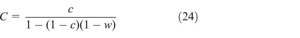
The coverage area of the joint nodes is bigger than the coverage area of the single nodes, so the C > W, that is

c > 1 - (\frac{1}{1 + w})

(26)

From the relevant knowledge of the probability theory, q ∈ [0,1], calculating the awareness intensity, when goal nodes are covered completely by single nodes, that is when w = 1, c > 1/2. The physical signification is that whether single nodes cover goal nodes or not, the awareness intensity of joint nodes holds more than 50% of the total, which verifies that the awareness intensity is higher than the single of that.

Redundancy coverage

At the initial time, the deployment of sensor nodes is casted in the monitoring area in high density and at random.^34–36 Because of the randomness, there will be plenty of redundancy nodes in somewhere of the monitoring area. The existence of large number of redundancy nodes will lower the network expansibility, cause the network congestion, and consume the network energy rapidly.^30,37,38 The solutions to solve the above-mentioned problems, there are two basic algorithms; they are the centralized optimization algorithm and the distributed optimization algorithm. The centralized optimization algorithm is mainly applied to the medium- and-small sized network system. The operating principle of it is that the sensor nodes compute their own geography information, the information will be uploaded to the sink nodes after the data fusion; the sink nodes will close or sleep the redundancy nodes to restrain the network energy consumption, after computing and analyzing the information collected. The distributed optimization algorithm is mainly applied to the large-scale sensor network. The operating principle of it is that after the mutual information of the sensor nodes and their neighbor nodes, the redundancy of the every node can be solved by a certain algorithm. When the redundancy is higher than the threshold value that is set in advance, the higher redundancy nodes will be closed or slept to save the network energy.^39–41 Compared with the centralized optimization algorithm, the applied range of the distributed optimization algorithm is higher; it can be widely used.

Definition 6 (redundancy coverage nodes)

Any two sensor nodes, s_i, s_j are the neighbor nodes to each other, when the Euclidean distance of the two nodes is smaller than the critical threshold ith that is called as the redundancy coverage nodes.

Definition 7 (redundant coverage)

When the sensor nodes s_i and the neighbor are the redundancy coverage nodes to each other, the specific value of the sensing area of sensor nodes s_i and neighbor nodes is the redundant coverage, we usually express it using P(α).

Definition 8 (connected graphs)

The Astatic connected graph, G, G = (V,E), is given, the sensor nodes s_i ∈ V, the connectivity d(u) of the nodes is defined as the number of the neighbor nodes; and the connectivity of the G is defined as the minimum of the nodes in the V.

Theorem 4

The redundant coverage of the n redundant nodes that belong to any one sensor node s_i needs to meet

\begin{array}{l} P (n) = \\ 1 - {1 - \frac{1}{π} [\frac{π}{4} - \frac{λ \sqrt{4 - k^{2}}}{8} + \frac{λ^{2}}{2} \arccos (\frac{λ}{2}) - \frac{λ^{3} \sqrt{4 - λ^{2}}}{16}]}^{n} \end{array}

Proof

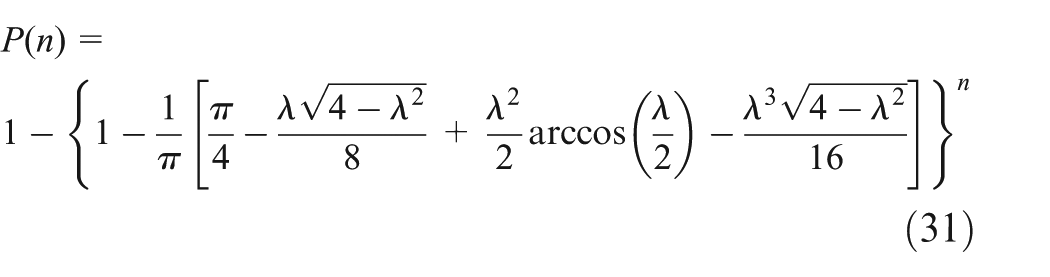
Taking Figure 2 as the example to prove this. According to the characteristic of the Poisson distribution, the distribution of the n redundant neighbor nodes of the sensor node s_i complies with uniform distribution. The sensor nodes are all homogeneous nodes, the proportional relation of the communication radius R with the perceived radius r is R = λr, where λ is coefficient of proportionality, supposing that ∠BCE = α; the distance between the point B and the point C is a random variable, according to the probability density function

f_{L} (x) = \frac{2 x}{λ^{2} r^{2}}, 0 \leq x \leq λ r

(27)

Figure 2.

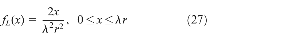
Node joint-coverage sketch.

The area of the intersection of the two circles S₁ can expressed as follows

S_{1} = (2 a - \sin 2 a) r^{2}

(28)

Making the distance between B and C, l = 2r cos α, dl = 2r sin αdα, $α \in [\arccos λ / 2, π / 2]$ , then put α into the probability formula, simplify the formula

\begin{array}{l} P_{a} = \int_{λ / 2}^{\arccos λ / 2} (2 α - \sin 2 α) \frac{4 r^{2} \cos α}{λ^{2}} \sin α d α \\ = \frac{1}{π} [\frac{π}{4} - \frac{λ \sqrt{4 - λ^{2}}}{8} + \frac{λ^{2}}{2} \arccos (\frac{λ}{2}) - \frac{λ^{3} \sqrt{4 - λ^{2}}}{16}] r^{2} \end{array}

(29)

According to formula (27), for any sensor node that covers the redundant neighbor nodes, the redundant coverage can be expressed as follows

\begin{array}{l} P_{b} = \frac{P_{a}}{π r^{2}} = \frac{1}{π^{2}} \\ [\frac{π}{4} - \frac{λ \sqrt{4 - λ^{2}}}{8} + \frac{λ^{2}}{2} \arccos (\frac{λ}{2}) - \frac{λ^{3} \sqrt{4 - λ^{2}}}{16}] \end{array}

(30)

That is that when there are n communication nodes covering any sensor nodes, the redundant coverage is as follows

\begin{array}{l} P (n) = \\ 1 - {1 - \frac{1}{π} [\frac{π}{4} - \frac{λ \sqrt{4 - λ^{2}}}{8} + \frac{λ^{2}}{2} \arccos (\frac{λ}{2}) - \frac{λ^{3} \sqrt{4 - λ^{2}}}{16}]}^{n} \end{array}

(31)

Steps and descriptions of CAOND algorithm

When the moving object entered the monitored area, active cluster head node around the target would monitor it first. The cluster head node sends on-duty messages to member nodes and neighbor nodes to awaken those member nodes to enter waiting state and notify the neighbor cluster head nodes the monitored information of the target. Based on the above information, member nodes calculate their weighting of whether participating the monitoring. If its weighting is greater than the set threshold, the node would enter into active state and monitor any moving target within its sensing range. Active nodes around the target will form an initial dynamic cover group. Member nodes will send an information packet to the cluster head node. The data packet contains information such as time stamp, node ID, and distance between the nodes and the target. As there may be more than one cluster head node in CAOND, for the convenience of management, one of the cluster head nodes will be selected as managing node, and it is responsible for the information fusion and data management. Because the target node is moving in the monitoring area, the initial CAOND may not meet the requirements of target monitoring. Therefore, dynamic reconstruction is needed according to the position of the target. Reconstruction process is completed by members updating management and head node re-selecting. When the target moves to a new grid, new cluster head node and member nodes will meet the threshold weighting joint to the original CAOND, the newly jointed cluster head node is elected as the leader node. Nodes of the original CAOND that cannot meet the monitoring requirements will quit the CAOND. If the original managing node happens to be a quitting one, at this time, the original managing node needs to send information of target location and information of member nodes to the new managing node. When the target moves away from the original location, the cluster head node will broadcast messages to its member nodes to enter into sleep state to save power consumption, Steps of the algorithm are as follows:

Step 1: Initialize the correlation parameters.

Step 2: Store the node information and the neighboring nodes in the s[i].data, including the information of the parameters, such as, the ID of the nodes, the left energy, coverage probability.

Step 3: Broadcast the information in the way of flooding, an undirected graph.

Step 4: When the energy of the node is more than the minimal energy, then the node will be started, be at the working state; if the energy of the node is smaller than or equal to the minimal energy, the node will be altered into the sleeping state, the basic information of the node will be recorded in the list, the neighboring node will be started.

Step 5: After all the working nodes have collected all the information of the relevant information, the current coverage probabilities will be evaluated to the corresponding nodes in the list.

Step 6: The indicator of the list will point the next node.

Step 7: When the energy of the current node is higher than that of the next node, then the sink node will send information to the node; calculate the coverage probability of the node, until all the nodes in the list have been traversed.

1 Procedure

2 Begin

3 n←Null //Initialization Parameters

4 CL←Null

5 While (i < n)

6 {

7 {

8 s[i].information→s[i].bata //Calculating the node information and storing them

9 s[i].neighbor.information→s[i].neighbor.bata

10 s[i].broadcast→Gn //sending the nodes to the sink node

11 }

12 ConstuctGraph() //building the connected graph

13 while(s[i].energy>=minenergy)

14 if(redundancy.nodes>=I_th) //the node energy no less than the threshold

15 Network_working

16 else

17 {

18 sorting(s[i].energy) //ranging them by the node energy

19 s[i].maxenergy→dormancy //sleeping the high-energy node

20 }

22 if(Gn←s[i].inf_coverage) //gathering and receiving the node information

23 {

24 CL[i]←s[i].inf_coverage //storing the received information to the List

25 i++ //pointing to the next nodes

26 }

27 if(s[i].energy>=s[i+1].energy)

28 {

29 Gn.inf_notice→s[i].data //the sink nodes sends and gets the present node the information

30 s[i].coverage→target.nodes //the present node covers the target node

31 }

32 }

Complexity of the CAOND algorithm

The algorithm is sending and receiving data in the way of single circle, so the complication of the algorithm is O(n); in the process of ranging the node energy, it is completed in the way of nested invocations of methods, so the complication of the algorithm is O(n²). Thus, based on above analysis, the complication of the CAOND in the article is O(n²).

Analysis of the coverage quality

When sensor nodes are working, the energy consumption is mainly caused by node awareness part and the communication part. In the awareness part, within one single circle, the energy consumption is caused by the node awareness collecting a bit data; in the communication part, the energy consumption is caused by the transmitting and receiving k bits under the condition of the distance of the neighbor node being d

E_{T} (k, d) = {\begin{matrix} E_{T - elec} k + ε_{fs} d^{2} k d < d_{0} \\ E_{R - elec} k + ε_{amp} d^{4} k d \geq d_{0} \end{matrix}

(32)

E_{R} (k) = E_{R - elec} k

(33)

In the formulas, the E_T-elec and the E_R-elec stand for the energies that are consumed when transmitting or receiving 1 bit data; the d₀ stands for the threshold of the Euclidean distance of the nodes and the communication neighbor nodes; the ε_amp stands for the quantity of the multiple attenuation energy consumption; the ε_fs stands for the energy of the nodes in the free space. When the nodes are transmitting the data, the indexes of the path attenuation energy are 2 and 4.

In order to verify the effectiveness and the feasibility of the CAOND, we take the MATLAB 7.0 as the simulation platform, take different scales of the monitoring area, and dynamic parameter as the research objective. Then, the contrast experiment is set to compare with Sun et al.,¹⁹ Yuchee et al.,²⁶ and Wang et al.²⁷ in terms of the node deployment, the network coverage ratio, the dynamic change of the sleeping redundant nodes, and the lifetime of the network. The values of every group data are taken from the mean values of 50 simulation data. The values of the simulation data can be seen in Table 2.

Table 2.

The specification of the simulation data.

The simulation data	The simulation values	The simulation data	The simulation values
The monitoring area I	100 × 100 m²	R	20 m
The monitoring area II	200 × 200 m²	E_R-elec	30 J/b
The monitoring area III	300 × 300 m²	E_T-elec	30 J/b
R	10 m	ε_fs	10 (J/b)/m²
N	1000	energy	2 J
ε_amp	10 (J/b)/m²	time	600 s
e_min	0.005 J	λ	0.8 or 1.2

Taking the adjoining sensor nodes as the research objective to confirm the value range of the probability density parameter λ, optimize the different simulations of domain. Supposing that the mean probability density of the sensor nodes in the monitoring area is λ, the Euler distance between the adjoining nodes is d; the perceived radius of the sensor nodes is equal to the sides of the external hexagonal that is the R_s (Figure 3).

Figure 3.

Model of the evenly distributed sensor nodes.

For the single sensor nodes, the functional relationship of the area of the regular hexagon and the probability density parameter can be expressed as follows

λ^{- 1} = 6 \times \frac{1}{2} \times R_{s} \times \frac{\sqrt{3}}{2} R_{s}

(34)

Putting formula (31) into $d = \sqrt{3} R_{s}$ and we get $d = \sqrt{2 \sqrt{3} / 3 λ}$ . In the wireless sensor network, the necessary of keeping the network connection is that the communication radius is equal or greater than the two times of the perceived radius, which is d ≤ 2R_s, after the calculation, the result is $λ \geq \sqrt{3} / 6 R_{s}^{2}$ . When the d < R_s, there will be plenty of the redundant nodes in the monitoring area, which can cause the rapid consumption of the node energy. In order to avoid the appearance of the situation, we optimize the network resources, making $λ \leq 2 \sqrt{3} / 3 R_{s}^{2}$ . To sum up the above-mentioned situations, the value range of the λ is $[\sqrt{3} / 6 R_{s}^{2}, 2 \sqrt{3} / 6 R_{s}^{2}]$ .

Experiment 1

When the value of λ is limited within the range, we take the simulation experiment in the monitoring area 300 × 300. The results are shown in Figures 4 –9.

Figure 4.

$λ < \sqrt{3} / 6 R_{s}^{2}$ , the coverage situation of random deployment in the initial time.

Figure 5.

$λ < \sqrt{3} / 6 R_{s}^{2}$ , the coverage situation of the CAOND.

Figure 6.

$\sqrt{3} / 6 R_{s}^{2} \leq λ \leq 2 \sqrt{3} / 6 R_{s}^{2}$ , the coverage situation of random deployment in the initial time.

Figure 7.

$\sqrt{3} / 6 R_{s}^{2} \leq λ \leq 2 \sqrt{3} / 6 R_{s}^{2}$ , the coverage situation of the CAOND.

Figure 8.

$λ > 2 \sqrt{3} / 3 R_{s}^{2}$ , the coverage situation of random deployment in the initial time.

Figure 9.

$λ > 2 \sqrt{3} / 3 R_{s}^{2}$ , the coverage situation of the CAOND.

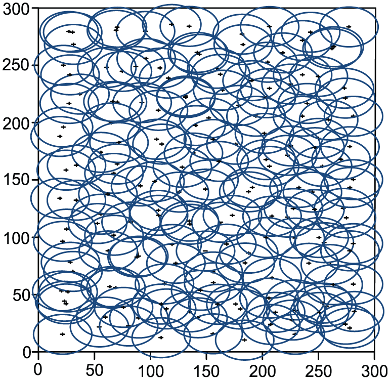
From Figures 4 –9, they provide the coverage situation of the random deployment coverage and the optimization of the CAOND when the values of the λ are different. After the calculation, when $λ < \sqrt{3} / 6 R_{s}^{2}$ , the coverage P = 69.32%, shown in Figure 5; in order to simplify the calculation, when $\sqrt{3} / 6 R_{s}^{2} \leq 2 \sqrt{3} / 6 R_{s}^{2}$ , putting the mean value into the calculation, which is when the $λ = 5 \sqrt{3} / 12$ , the coverage ratio P = 86.28%, as it is shown in Figure 7; when the $λ > 2 \sqrt{3} / 3 R_{s}^{2}$ , the coverage ratio P = 98.11%, as it is shown in Figure 9. Having compared Figure 4 with Figure 9, the coverage ratio of Figure 9 is much higher than that of Figure 5 and Figure 7. Although the requirements of the redundancy can be met in Figure 5, the coverage ratio is lower, which cannot achieve the effective coverage. The existence of the redundant nodes will cause large consumption of the network energy, lower the energy of the whole network. Meanwhile, it will cause heavier interference to the communication linkage of the network. However, Figure 5 can meet the requirements of the redundancy, but it has a low coverage probability and cannot meet the effective coverage; meanwhile, it will cause lots of coverage holes, which is not benefit to the effective coverage of the monitoring area. According to Figure 7, the optimized deployment of the nodes has been completed, the deployment of the nodes is homogeneous, the coverage probability can reach 86.82%, and the number of the redundant nodes is far less than that of Figure 9, which finally extend the lifetime of the network. In summary, the more ideal situation is shown in Figure 7.

Experiment 2

Using different scale of the simulation platform, we compare the CAOND in this article with Bachir et al.¹³ and Meng et al.²¹ in terms of the coverage ratio and the quantity of the redundant nodes. The results can be shown in Figures 10 –15.

Figure 10.

100 × 100 m², quantity comparison of the sensor nodes and work nodes.

Figure 11.

200 × 200 m², changing curve of network coverage probability.

Figure 12.

300 × 300 m², the comparison of the CAOND under different coverage probabilities.

Figure 13.

300 × 300 m², comparison of the quantity of the redundant sensor nodes and the coverage probability.

Figure 14.

300 × 300 m², quantity comparison of the sleeping redundant nodes and the coverage.

Figure 15.

300 × 300 m², quantity comparison of the redundant nodes and the sleeping nodes.

From Figures 10 –15, they provide the changing curves of the coverage ratio, the changing curves of the redundant nodes quantity, and the coverage ratio in the case of different network scales. Figure 10 provides the changing curves of the quantity of the sensor nodes, the sensor work nodes in the CAOND as well as the SCA and the EPDM. From Figure 10, we can know that the CAOND in this article needs less work nodes under the function of different parameters; however, the EPDM needs more sensor nodes.

The reason is that when the λ = 1.2, the coverage area that the sensor nodes and the neighbor nodes forms is bigger than that when λ = 0.8. However, the SCA and the EPDM achieve the effective coverage of the monitoring area by adding the quantity of the sensor nodes. The increase in number of the sensor nodes will produce lots of redundant nodes, and it will cause rapid consumption of the energy of the sensor nodes, which is not benefit to the balance of the whole network energy. Figure 11 chooses the 200 × 200 m² as the simulation platform, provides the changing curves of the coverage ratio changing with the change of the sensor nodes. From Figure 11, when the quantity of the sensor nodes is adding, the coverage ratio of the three algorithms is improving. In this article, the CAOND adjusts the coverage by setting the dynamic parameter λ. So at the initial time, the coverage ratio of the CAOND is higher than that of the other two algorithms. When the quantity of the sensor nodes is 137, the algorithm in this article can achieve the effective coverage; however, the SCA and the EPDM can achieve the effective coverage when the quantities are 188 and 199. Compared with the two algorithms, the mean coverage ratio of the CAOND has improved 13.36% on average. The main reason is that CAOND algorithm uses the setup of the parameter λ to adjust the number of the working nodes, makes more nodes cover the goal nodes by the round scheduling system, which will prolong the network lifetime. From Figures 12 –15, they choose the 300 × 300 m² as the simulation platform, provide the comparison of the different coverage ratios, and the quantity of the redundant nodes. From Figure 12, we can get to know that having met the certain coverage ratio, the bigger the value of λ is, the less the quantity of the sensor nodes is. The reason is similar to the analysis of Figure 7. Figure 13 provides the contrast diagram of the redundant sensor nodes and the coverage ratio. From Figure 13, we can get that when the redundant nodes are increasing, the coverage ratio is declining. It mainly because the EPDM completes the dispatch of the status of the redundant nodes in the way of probability driven; however, the SCA completes the process of the receivingand transmitting the information among the nodes. CAOND algorithm uses the coverage capability of the nodes to reduce the number of the working nodes; thus, the purpose of saving the energy of the sensor nodes can be reached. However, SCA algorithm and EPDM algorithm use the technology of global information to complete the coverage of the monitoring area; they complete the coverage by increasing the number of the sensor nodes, which is not suitable for the limited resource of the wireless sensor network. The analysis of Figures 14 and 15 is similar to that of Figures 11 and 12.

Experiment 3

In different simulation scales, the contrast experiment is taken between the CAOND and the ECTA. Sahoo and Sheu²⁰ propose in terms of the lifetime of the network and the runtime of the algorithms.

Figures 16 and 17 provide the comparison of the CAOND and the ECTA in terms of the lifetime of the network and the runtime of the algorithms. From Figure 16, we can get that at the initial time, the network lifetime of the two algorithms is almost equal to each other; as the quantity of the sensor nodes is increasing, the network lifetime of them is increasing. However, the ECTA monitors the nodes by the nonlinear continuous coverage pattern, so the energy consumption is higher than the CAOND. When the quantity of the sensor nodes is 180, the network lifetime of the two algorithms is going to be steady, and the mean network lifetime of the CAOND is 12.92% higher than the ECTA. Figure 17 provides the contrast diagram of the quantity of sensor nodes and the runtime of the algorithm. The ECTA adopts the chain list storage to store the node energy, ranges the node from the highest to the lowest by the traversal algorithm, making the high-energy nodes get the higher authority to complete the coverage of the target node. The complication of the ECTA is lower than the CAOND. So, in terms of the runtime, the runtime of the CAOND is higher than the ECTA.

Figure 16.

200 × 200 m², comparison of the network lifetime of the two algorithms.

Figure 17.

Comparison of the runtime of the two algorithms.

Conclusion

In order to solve the issue of the wireless sensor network coverage better, on the basis of its characteristics, the article proposes the optimization coverage algorithm of the dynamic parameters of the controlled. The algorithm gives the solving method of the maximum coverage area of the three-circle seamless joint first. Second, taking advantages of the related theory of the probability to solve the expected value of the coverage quality in the monitoring area, based on which provide the solving method to the minimum quantity of the sensor nodes. On the basis of the analysis of the node coverage, this article provides the comparison and contrast of the awareness intensity of the joint nodes and the single nodes. In terms of researching the redundant nodes coverage, the article has proved the condition that there is redundant coverage in the sensor nodes; this article provides the steps and descriptions how to suppress the consumption of the energy in detail; finally, through the simulation experiment, the algorithm in this article has been simulated in terms of the optimization deployment, the coverage rate, the redundancy rate, and the network lifetime as well as the runtime of the algorithm. The analysis and the expression of the simulation result show the effectiveness and the feasibility of the CAOND in this article. The future work may focus on how to realize the effective coverage of the boundary boxes and the effective coverage of the multiple moving target nodes.

Footnotes

Academic Editor: Wei Yu

Declaration of conflicting interests

The author(s) declared no potential conflicts of interest with respect to the research, authorship, and/or publication of this article.

Funding

The author(s) disclosed receipt of the following financial support for the research, authorship, and/or publication of this article: This work was supported by the National Natural Science Foundation of China under Grant No. 61503174 and 61628210; Henan Province Education Department Natural Science Foundation under Grant No. 15A413016, 16A520063, and 17A520044; Natural Science and Technology Research of Henan Province Department of Science Foundation under Grant No. 142102210063, 152102410053, 162102210113, 162102210276, and 162102410051; Henan Province Education Department Cultivation Young Key Teachers in University of Under Grant No. 2016GGJS-158; the Guangdong Natural Science Foundation of China under Grant No. 2016A030313540, and Guangzhou Education Bureau Science Foundation under Grant No. 1201430560, Shaanxi Education Bureau Science Foundation under Grant No. 2016SF-428; Science and Technology Development Project of Luoyang Foundation under Grant No. 1401037A.

References

Erdelj

Loscri

Natalizio

. Multiple point of interest discovery and coverage with mobile wireless sensor. Ad Hoc Netw 2013; 11(8): 2288–2300.

Iqbal

Naeem

Anpalagan

. Wireless sensor network optimization: multi-objective paradigm. Sensor 2015; 15(7): 17572–17620.

Ahmadi

Shojafar

Hajeforosh

. An efficient routing algorithm to preserve k-coverage in wireless sensor networks. The J Supercomput 2014; 68(2): 599–623.

Yoon

Kim

YH.

An efficient genetic algorithm for maximum coverage deployment in wireless sensor networks. IEEE T Cybern 2013; 43(5): 1473–1483.

Zheng

Xiao

Wang

. Capacity and delay analysis for data gathering with compressive sensing in wireless sensor networks. IEEE T Wirel Commun 2013; 12(2): 917–918.

Wang

Chin

Soh

On minimizing data forwarding schedule in multi transmit/receive wireless mesh networks. IEEE Access 2016; 4: 1570–1582.

Cheng

Leung

Maupin

A delay-aware network structure for wireless sensor networks with in-network data fusion. IEEE Sens J 2013; 13(5): 1622–1631.

Zairi

Zouari

Niel

. Nodes self-scheduling approach for maximizing wireless sensor networks lifetime based on remaining energy. IET Wirel Sens Syst 2012; 2(1): 52–62.

Zhu

Nii

. PaperIO: a 3D interface towards the internet of embedded paper-craft. IEICE T Inf Syst 2014; E97-D(10): 2597–2605.

10.

Derr

Manic

Wireless sensor network configuration—part II: adaptive coverage for decentralized algorithms. IEEE T Ind Inform 2013; 9(3): 1728–1738.

11.

Zhu

Zhang

. Collaborative wireless sensor networks and applications. Int J Distrib Sens Netw 2015; 11: 1–2.

12.

Aliouat

Naidja

. Adaptive nodes diagnosis and recovery for wireless sensor networks. In: Proceedings of the 2012 international symposium on computer applications and industrial electronics (ISCAIE), Kota Kinabalu, Malaysia, 3–4 December 2012, pp.256–261. IEEE.

13.

Bachir

Bechkit

Challal

. Joint connectivity-coverage temperature-aware algorithms for wireless sensor networks. IEEE T Parallel Distrib Syst 2015; 26(7): 1923–1936.

14.

Sun

Zhang

Xing

. EBKCCA: a novel energy balanced k-coverage control algorithm based on probability model in wireless sensor networks. KSII T Internet Inf Syst 2016; 10(8): 3621–3640.

15.

Naranjo

PGV

Shojafar

Mostafaei

. P-SEP: a prolong stable election routing algorithm for energy-limited heterogeneous fog-supported wireless sensor networks. J Supercomput 2016; 73: 733–755.

16.

Adulyasas

Sun

Wang

Connected coverage optimization for sensor scheduling in wireless sensor networks. IEEE Sens J 2015; 15(7): 3877–3892.

17.

Sun

Wang

. An enhanced coverage control algorithm for wireless sensor networks based on adjustable parameters. Acta Electron Sin 2015; 43(7): 466–474.

18.

Liao

Wang

Zhang

. Minimizing movement for target coverage and network connectivity in mobile sensor networks. IEEE T Parallel Distrib Syst 2015; 26(7): 1971–1983.

19.

Sun

Wang

. ECAPM: an enhanced coverage algorithm in wireless sensor networks based on probability model. Int J Distrib Sens Netw 2015; 2015(1): 1–11.

20.

Sahoo

Sheu

JP.

Limited mobility coverage and connectivity maintenance protocols for wireless sensor networks. Comput Netw 2011; 55(13): 2856–2872.

21.

Meng

Wang

Connected coverage protocol using cooperative sensing model for wireless sensor networks. Acta Electron Sin 2011; 39(4): 772–779.

22.

Mini

Siba

Samrat

LS.

Sensor deployment and scheduling for target coverage problem in wireless sensor networks. IEEE Sens J 2014; 14(3): 636–644.

23.

. Transforming complete coverage algorithms to partial coverage algorithm for wireless sensor networks. IEEE T Parallel Distrib Syst 2011; 22(4): 695–703.

24.

Zhao

Liu

. Optimization strategy on coverage control in wireless sensor network based on Voronoi. J Commun 2013; 28(1): 36–43.

25.

Hanid

Kaveh

Amir

. Distributed deployment algorithms for improved coverage in a network of wireless mobile sensors. IEEE T Ind Inform 2014; 10(1): 163–174.

26.

Yuchee

Poyu

Wentsuen

k-Angle object coverage problem in a wireless sensor network. IEEE Sens J 2012; 12(12): 3408–3416.

27.

Wang

Liao

Cao

. Achieving k-barrier coverage in hybrid directional sensor networks. IEEE T Mob Comput 2014; 13(7): 1443–1455.

28.

Xing

Wang

Polytype target coverage scheme for heterogeneous wireless sensor networks using linear programming. Wirel Commun Mob Comput 2014; 14(14): 1397–1408.

29.

Sun

Wang

. A novel coverage algorithm based on event-probability-driven mechanism in wireless sensor network. EURASIP J Wirel Commun Netw 2014; 2014: 1–17.

30.

Tseng

Cho

Chou

. Efficient power conservation mechanism in spline function defined WSN terrain. IEEE Sens J 2014; 14(3): 853–864.

31.

Pan

Maximum lifetime scheduling for target coverage and data collection in wireless sensor networks. IEEE T Veh Technol 2015; 64(2): 714–727.

32.

Sun

Zhao

Chen

. Effective link interference model in topology control of wireless ad hoc and sensor networks. J Netw Comput Appl 2015; 52: 69–78.

33.

Wang

Meng

ZZ.

Energy efficient coverage conserving protocol for wireless sensor networks. J Softw 2010; 21(12): 3124–3137.

34.

Ammari

Das

SK.

Centralized and clustered k-coverage protocols for wireless sensor networks. IEEE T Comput 2012; 61(1): 118–132.

35.

Otero

Haber

Peter

. A wireless sensor network’s analytics system for predicting performance in on-demand deployments. IEEE Syst J 2012; 9(4): 118–132.

36.

Menegazzo

Albini

LC.

Unadvertised energy saving method for static and homogeneous wireless sensor networks. IET Wirel Sens Syst 2014; 4(3): 105–111.

37.

Halder

Bit

SD.

Enhancement of wireless sensor network lifetime by deploying heterogeneous nodes. J Netw Comput Appl 2014; 38: 106–124.

38.

Zhang

Liu

Samani

. Cooperative spectrum sensing in cognitive wireless sensor networks. Int J Distrib Sens Netw 2015; 2015: 1–15.

39.

Sun

Wang

. A novel energy-efficient k-coverage algorithm based on probability driven mechanism of wireless sensor networks. Int J Distrib Sens Netw 2016; 2016(1): 1–9.

40.

Wong

Siew

Yoong

. Node collaboration for distributed beam forming in wireless sensor networks. In: Proceedings of the 2012 IEEE international conference on control system, computing and engineering, Penang, Malaysia, 23–25 November 2012, pp.483–488. New York: IEEE.

41.

Gong

Yang

YY.

Low-latency SINR-based data gathering in wireless sensors networks. IEEE T Wirel Commun 2014; 13(6): 3207–3221.