Assessment of in Partially Linear Logistic Regression with Missing and Complete Data

Abstract

Generalized partially linear models (GPLMs) provide a versatile regression framework that blends parametric and nonparametric components, allowing flexible modeling of complex data structures. In binary response settings, particularly within logistic frameworks, verifying the independence between covariates and error terms is essential for ensuring model adequacy and validity. This paper develops a nonparametric diagnostic based on the Bergsma–Dassios measure of association, $τ^{*}$ , to assess the independence between the regressors $(X, W)$ and the random error component in logistic GPLMs. Unlike traditional correlation measures, $τ^{*}$ captures broad classes of dependencies, including nonlinear and nonmonotonic associations, thus offering a powerful and robust diagnostic tool. Both complete data and missing-response scenarios are considered, where responses are missing completely at random (MCAR) or missing at random (MAR). Consistent and asymptotically efficient estimators for the parametric vector $β$ and the nonparametric function $m (W)$ are constructed under these settings. Theoretical properties of the proposed $τ^{*}$ -based test are established, including its asymptotic distribution and power against local alternatives. Simulation studies and real-data analyses further confirm the practical effectiveness and robustness of the proposed method, demonstrating its utility in semiparametric logistic regression with incomplete or potentially misspecified data.

Keywords

partially linear logistic regression semiparametric models Bergsma–Dassios independence testing missing data MCAR MAR kernel smoothing B-splines,U-statistics

1. Introduction

Generalized partially linear models (GPLMs) constitute an important class of semiparametric models that blend the simplicity and interpretability of linear models with the flexibility of nonparametric techniques (Härdle, 2004; Hastie & Tibshirani, 1990; Ruppert et al., 2003). In numerous fields—such as epidemiology, economics, and biostatistics—analysts often encounter datasets where some covariates affect the outcome in a linear manner, while others have nonlinear or unspecified influences. The GPLM framework elegantly addresses this challenge by expressing the conditional probability of the binary response variable as

P (Y = 1 ∣ X, W) = {1 + \exp [- (X^{⊤} β + m (W))]}^{- 1},

where

X \in R^{p}

denotes the set of covariates with linear effects,

W \in R^{q}

represents covariates with nonlinear contributions captured by the unknown smooth function

m (\cdot)

, and

Y \in {0, 1}

is the binary response. This logistic partially linear specification is particularly advantageous in medical and social science studies, where the underlying dependence structure between covariates and the outcome is intricate and only partially understood.

Recent work in semiparametric regression diagnostics has focused on developing nonparametric tests for model adequacy and dependence structures that go beyond classical approaches. For example, innovative nonparametric specification tests have been proposed for semiparametric regression models using residual transformations and spectral decompositions (Ferraccioli et al., 2023), and distance-based measures have been used to test conditional variance structures in regression models (Hu et al., 2024). Methods for testing independence in complex data structures such as sparse longitudinal data also illustrate ongoing interest in powerful, general dependence testing beyond simple correlation measures (Zhu et al., 2024). In the presence of spatial dependence, the adequacy of a parametric regression model can be assessed by contrasting it with a flexible nonparametric alternative through an $L^{2}$ -distance–based goodness-of-fit framework, as proposed by Meilán-Vila et al. (2020). These developments underline the relevance and timeliness of exploring $τ^{*}$ as a diagnostic tool in generalized partially linear models.

A key yet often overlooked assumption in regression modeling is the independence between covariates and the error term. Violation of this assumption can severely bias parameter estimation, affect prediction accuracy, and compromise inference validity. Traditional residual-based diagnostics or correlation measures such as Pearson’s $ρ$ or Spearman’s $ρ_{S}$ may fail to detect complex, nonlinear associations, especially in high-dimensional or semiparametric settings (Bergsma & Dassios, 2014; Székely et al., 2007).

To address this, we study a recently proposed nonparametric dependence measure, $τ^{*}$ , introduced by Bergsma and Dassios (Bergsma & Dassios, 2014), which generalizes Kendall’s tau and is zero if and only if the variables are independent under very broad conditions (Newey, 1994). This makes $τ^{*}$ particularly well-suited for assessing whether regressors $(X, W)$ are associated with the model’s error component, thus offering a powerful diagnostic tool for model adequacy.

In this paper, we integrate $τ^{*}$ into the logistic GPLM framework and study its properties under two practical data settings:

(i)
The response variable $Y$ is fully observed for all observations.
(ii)
The response variable $Y$ is subject to missingness, either completely at random (MCAR) or at random (MAR), as defined by Rubin (1976).

In both cases, we develop estimation strategies for the parameter vector $β$ and the unknown function $m (\cdot)$ that are robust, consistent, and efficient. For the missing data scenario, inverse probability weighting (IPW) and likelihood-based methods are employed to adjust for the missingness mechanism (Little & Rubin, 2002; Tsiatis, 2006).

Our empirical analysis on several real datasets illustrates the practical performance of $τ^{}$ as a model-checking tool. In particular, $τ^{}$ provides evidence for or against the assumption of independence between predictors and errors, guiding researchers in refining model specifications or addressing potential misspecifications.

The rest of the paper is organized as follows: Section 2 outlines the model setup and introduces the $τ^{}$ statistic; Section 3 describes the estimation procedures under both full and missing data settings; Section 4 discusses theoretical properties and asymptotics of $τ^{}$ ; Section 5 elaborates the asymptotic power determination of $τ^{*}$ under contiguous alternatives; Section 6 presents simulation studies and real-data applications; and Section 7 concludes with a discussion and future directions.
2. Model Setup

We consider a binary response variable $Y \in {0, 1}$ modeled through a generalized partially linear logistic regression framework. The covariate vector is partitioned into two components: $X \in R^{p}$ , which enters the model linearly, and $W \in R^{q}$ , whose effect is modeled nonparametrically via an unknown smooth function $m (\cdot)$ . The conditional success probability is specified as

P (Y = 1 ∣ X, W) = {1 + \exp [- (X^{⊤} β + m (W))]}^{- 1},

(2.1)

where

β \in R^{p}

is an unknown finite-dimensional parameter vector and

m : R^{q} \to R

is an unknown smooth function capturing potentially nonlinear effects of

W

This specification combines the interpretability of generalized linear models with the flexibility of nonparametric regression and is widely used in applications in biostatistics, epidemiology, and the social sciences (Hastie & Tibshirani, 1990; Ruppert et al., 2003).

Let ${(Y_{i}, X_{i}, W_{i})}_{i = 1}^{n}$ denote an independent and identically distributed sample from the joint distribution of $(Y, X, W)$ . Throughout the paper, we impose the following regularity assumptions, which are standard in the analysis of semiparametric partially linear models.

(A1)

The covariate vectors $X_{i} \in R^{p}$ and $W_{i} \in R^{q}$ are observed for all $i$ and have a joint density supported on a compact subset of $R^{p + q}$ . In particular, the support of $W$ is bounded.

(A2)

The unknown function $m (\cdot)$ is sufficiently smooth; specifically, $m$ possesses continuous partial derivatives up to the order required by the kernel- or spline-based estimation procedures employed in this paper.

(A3)

The logistic link function in (2.1) is correctly specified.

(A4)

The kernel function $K (\cdot)$ used for estimating conditional expectations is symmetric, bounded, integrates to one, and has finite second moments.

(A5)

The bandwidth parameters $h_{1}, \dots, h_{q}$ satisfy $h_{l} \to 0$ as $n \to \infty$ for each $l = 1, \dots, q$ , and $n h_{1} \dots h_{q} \to \infty$ .

(A6)

(Identifiability) The nonparametric component satisfies the normalization constraint $E {m (W)} = 0$ .

Assumptions (A1)–(A6) are standard in semiparametric partially linear models and ensure the identifiability, consistency, and asymptotic normality of the estimators developed in the subsequent sections, as well as the validity of the proposed independent diagnosis based on $τ^{*}$ .

In subsequent sections, we address estimation of both components— $\underset{\sim}{β}$ and $m (\cdot)$ —under two contexts: (i)

When the data is fully observed (no missingness).

(ii)

When some responses $Y_{i}$ are missing, either completely at random (MCAR) or at random (MAR) (Rubin, 1976).

We further define a residual-like quantity $δ_{i} = Y_{i} - π_{i}$ , where $π_{i} = P (Y_{i} = 1 ∣ X_{i}, W_{i})$ , and introduce the dependence measure $τ^{*}$ to test whether these residuals are independent of the covariates. The model adequacy, estimation efficiency, and implementation details of the proposed approach are discussed in the following sections.

3. Estimation of Model

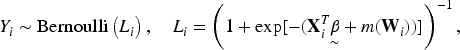
The underlying logistic regression model is expressed as

Y = L (X, W) + ϵ, where L (X, W) = {1 + \exp [- (X^{⊤} β + m (W))]}^{- 1} .

(3.1)

The random error

ϵ

takes the values

(1 - L (X, W))

- L (X, W)

depending on whether

Y = 1

Y = 0

, with corresponding probabilities

L (X, W)

and

1 - L (X, W)

, respectively. Under the null hypothesis of correct model specification, these probabilities fully characterize the distribution of

ϵ

To facilitate estimation of the parametric and nonparametric components, we adopt a working partially linear representation based on the logit transformation of the success probability. This representation is used solely for estimation purposes and follows the classical approach of Robinson (1988) in semiparametric regression.

3.1. Estimation of

β

Corresponding to (3.1), the model can be written in the partially linear form

\tilde{Y} = \log (\frac{L (X, W)}{1 - L (X, W)}) = β^{⊤} X + m (W) + ϵ^{*},

(3.2)

where

\tilde{Y}

denotes a working latent response and

ϵ^{*}

is an unobserved error term introduced by the logit transformation. The observed binary response satisfies

Y = I (\tilde{Y} > 0)

, where

I (\cdot)

is the indicator function.

The latent formulation in (3.2) provides a convenient framework for estimating $β$ and $m (\cdot)$ using partialling-out techniques, even though $\tilde{Y}$ and $ϵ^{*}$ are not directly observed. This approach does not alter the underlying likelihood-based model in (3.1) but enables the application of standard semiparametric estimation theory.

We assume the usual partially linear model error conditions:

E (ϵ^{*} ∣ X, W) = 0, E (ϵ^{* 2} ∣ X, W) = σ^{2} (X, W) > 0.

Following the classical approach by Robinson (1988), we eliminate the nonparametric component by taking conditional expectations. From (3.2), take conditional expectation with respect to $W$ :

E (\tilde{Y} ∣ W) = \sum_{j = 1}^{p} β_{j} E (X_{j} ∣ W) + m (W) + E (ϵ^{*} ∣ W),

(3.3)

and observe that

E (ϵ^{*} ∣ W) = 0

by iterated expectations.

Subtracting (3.3) from (3.2), the nonparametric term $m (W)$ is removed:

\tilde{Y} - E (\tilde{Y} ∣ W) = \sum_{j = 1}^{p} β_{j} (X_{j} - E (X_{j} ∣ W)) + ϵ^{*},

or in vector form,

{\tilde{Y}}_{demeaned} = {\underset{\sim}{β}}^{T} [X - E (X ∣ W)] + ϵ^{*} .

Denote

{\tilde{Y}}_{demeaned} = \tilde{Y} - E (\tilde{Y} ∣ W), X_{j; demeaned} = X_{j} - E (X_{j} ∣ W), j = 1, \dots, p,

and collect these into matrices to write the regression.

{\tilde{Y}}_{demeaned} = X_{demeaned} \underset{\sim}{β} + {\underset{\sim}{ϵ}}^{*} .

(3.4)

The infeasible estimator for $\underset{\sim}{β}$ is

\hat{\underset{\sim}{β}} = {(X_{demeaned}^{T} X_{demeaned})}^{- 1} X_{demeaned}^{T} {\tilde{Y}}_{demeaned} .

(3.5)

provided that the matrix is full rank.

Since $E (\cdot ∣ W)$ is unknown, we estimate it using the Nadaraya-Watson kernel estimator:

\hat{E} (X_{k} ∣ W = w) = \frac{\sum_{m = 1}^{n} [\prod_{l = 1}^{q} \frac{1}{h_{l}} K_{l} (\frac{w_{l} - W_{m l}}{h_{l}})] X_{m k}}{\sum_{m = 1}^{n} \prod_{l = 1}^{q} \frac{1}{h_{l}} K_{l} (\frac{w_{l} - W_{m l}}{h_{l}})} .

(3.6)

and similarly for

E (\tilde{Y} ∣ W)

Replacing conditional expectations with their estimators yields the feasible estimator.

\tilde{\underset{\sim}{β}} = {({\hat{X}}_{demeaned}^{T} {\hat{X}}_{demeaned})}^{- 1} {\hat{X}}_{demeaned}^{T} {\tilde{Y}}_{demeaned} .

(3.7)

3.2. Estimation of

m (\cdot, \dots, \cdot)

After estimating $\underset{\sim}{β}$ , the function $m (W)$ is estimated from

m (W) = E (\tilde{Y} ∣ W) - {\underset{\sim}{β}}^{T} E (X ∣ W),

using kernel smoothing as above:

\hat{m} (w) = \hat{E} (\tilde{Y} ∣ W = w) - {\tilde{\underset{\sim}{β}}}^{T} \hat{E} (X ∣ W = w) .

3.2.1. Under No Missing Response Setup

The above estimators are directly applicable when all responses $Y_{i}$ are observed.

3.2.2. Under MCAR Response Setup

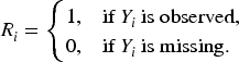
In many practical situations, some responses $Y_{i}$ may be missing completely at random (MCAR). Let $R_{i}$ denote the response missingness indicator, defined as

R_{i} = {\begin{cases} 1, & if Y_{i} is observed, \\ 0, & if Y_{i} is missing . \end{cases}

Assumption (M1) (MCAR). The missingness mechanism satisfies

P (R_{i} = 1 ∣ Y_{i}, X_{i}, W_{i}) = P (R_{i} = 1),

that is, the probability of observing the response does not depend on either observed or unobserved data.

Under Assumption (M1), valid inference can be based on complete cases or on inverse probability weighting schemes. For semiparametric models, incorporating the known or estimable missingness mechanism can improve efficiency (Rotnitzky & Robins, 1995).

3.2.3. Under MAR Response Setup

We now consider the more general missing-at-random (MAR) mechanism.

Assumption (M2) (MAR). The response missingness satisfies

P (R_{i} = 1 ∣ Y_{i}, X_{i}, W_{i}) = P (R_{i} = 1 ∣ X_{i}, W_{i}),

so that missingness may depend on observed covariates but not on the unobserved response, conditional on the observed data.

Under Assumption (M2), complete-case analysis may be biased, and consistent estimation requires the use of weighting or imputation techniques. In particular, inverse probability weighting and imputed local polynomial smoothing methods (Efromovich, 2011) provide asymptotically efficient estimation in this setting.

3.3. Estimation of $m (W)$ Under Missing Data

3.3.1. By Local Polynomial Smoothing

Local polynomial smoothing (LPS) is a widely used nonparametric regression technique that estimates the regression function $m (W)$ by fitting a polynomial locally around each target point $w \in R^{q}$ . The method generalizes kernel regression by approximating $m (\cdot)$ locally with a polynomial of degree $d$ instead of a constant.

Suppose we observe a sample ${(W_{i}, {\tilde{Y}}_{i})}_{i = 1}^{n}$ , where ${\tilde{Y}}_{i}$ are responses related to predictors $W_{i} = (W_{i 1}, \dots, W_{i q})^{T}$ .

The local polynomial estimator $\hat{m} (w)$ of order $d$ is obtained by solving

\hat{β} (w) = \arg min_{β \in R^{M}} \sum_{i = 1}^{n} K_{H} (W_{i} - w) {[{\tilde{Y}}_{i} - p_{d} (W_{i} - w)^{T} β]}^{2},

(3.8)

where

p_{d} (u)

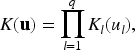
is the vector of all polynomial terms in

u_{1}, \dots, u_{q}

up to total degree

d

(e.g., for

q = 1

and

d = 1

p_{1} (u) = (1, u)^{T}

M = (\binom{q + d}{d})

is the dimension of the polynomial basis, and

K_{H} (u) = | H |^{- 1} K (H^{- 1} u)

is a multivariate kernel with bandwidth matrix

H

K (\cdot)

is a kernel function, typically a product of univariate symmetric kernels such as Gaussian kernels.

The estimator of the regression function at $w$ is

\hat{m} (w) = {\hat{β}}_{0} (w),

the first component of

\hat{β} (w)

, corresponding to the intercept term.

Kernel and Bandwidth Choice

The kernel $K$ is generally a symmetric density function, e.g.,

K (u) = \prod_{l = 1}^{q} K_{l} (u_{l}),

where each

K_{l}

is a univariate kernel.

The bandwidth matrix $H$ controls the smoothing degree. It can be chosen as a diagonal matrix with positive entries $h_{1}, \dots, h_{q}$ , called bandwidth parameters for each coordinate.

Optimal bandwidth selection can be done via cross-validation or plug-in methods to balance bias and variance.

No Missing Data Case

When all ${\tilde{Y}}_{i}$ are observed, the estimator (3.8) is computed using the full data. This yields a consistent and asymptotically normal estimator of $m (w)$ under standard regularity conditions (Fan, 2018).

MCAR (Missing Completely At Random) Case

If some responses are missing completely at random (MCAR), i.e., the missingness is independent of both observed and unobserved data, the local polynomial estimator can be applied using only complete cases:

{(W_{i}, {\tilde{Y}}_{i}) : R_{i} = 1},

where

R_{i}

is the indicator that

{\tilde{Y}}_{i}

is observed.

The estimator becomes

{\hat{β}}_{M C A R} (w) = \arg min_{β} \sum_{i = 1}^{n} R_{i} K_{H} (W_{i} - w) {[{\tilde{Y}}_{i} - p_{d} (W_{i} - w)^{T} β]}^{2} .

Although unbiased, this approach may be inefficient due to reduced sample size.

MAR (Missing At Random) Case

When missingness depends on observed data (MAR), ignoring missingness leads to bias. To correct for this, inverse probability weighting (IPW) or imputation methods are incorporated.

Inverse Probability Weighting (IPW): Let $π (Z_{i}) = P (R_{i} = 1 ∣ Z_{i})$ denote the probability that response $i$ is observed given covariates $Z_{i}$ (which may include $W_{i}$ and/or other variables). Assume $π (Z_{i})$ is estimable, e.g., via logistic regression.

The IPW local polynomial estimator solves

{\hat{β}}_{M A R} (w) = \arg min_{β} \sum_{i = 1}^{n} \frac{R_{i}}{\hat{π} (Z_{i})} K_{H} (W_{i} - w) {[{\tilde{Y}}_{i} - p_{d} (W_{i} - w)^{T} β]}^{2} .

The weight

\frac{R_{i}}{\hat{π} (Z_{i})}

corrects for bias introduced by missingness related to

Z_{i}

Missing at random and model validity. In the missing at random (MAR) framework, the probability that a response is missing may depend on the observed covariates but not on the unobserved response itself, conditional on the observed data. Formally, letting $R$ denote the missingness indicator, the MAR assumption implies $Pr (R = 1 ∣ Y, X, W) = Pr (R = 1 ∣ X, W)$ . Under this assumption, valid inference for the proposed $τ^{*}$ -based diagnostic relies on correct specification of the missingness mechanism through the response observation model. In particular, the consistency of the inverse probability weighting (IPW) and augmented IPW (AIPW) procedures used in this work depends on accurate modeling of the response probabilities; misspecification of the missingness model may lead to biased weights and consequently distort the resulting independence assessment.

ii.

Imputation-based methods: Alternatively, missing responses can be imputed using methods such as local linear smoothing, kernel regression, or model-based predictions before applying local polynomial smoothing on the completed dataset.

For example, under the imputed local linear smoothing (ILLS) approach (Efromovich, 2011), the missing ${\tilde{Y}}_{i}$ are replaced by estimated conditional expectations given the observed covariates, then the smoothing is applied as usual.

The choice of bandwidths $H$ is critical for balancing bias and variance and may differ under missing data mechanisms. Variance estimation and confidence interval construction under missing data require adjustment to account for weighting or imputation uncertainty.

3.3.2. By B-spline Regression

B-spline regression is a powerful nonparametric technique to estimate the smooth function $m (W)$ by representing it as a linear combination of basis spline functions. This approach offers flexibility in capturing complex relationships and can be adapted to handle missing data scenarios effectively.

Model Formulation

Express the function $m (W)$ as

m (W) \approx \sum_{j = 1}^{J} θ_{j} B_{j} (W),

where

{B_{j} (\cdot)}_{j = 1}^{J}

are B-spline basis functions defined over a suitable partition of the domain of

W

, and

θ = (θ_{1}, \dots, θ_{J})^{T}

is the vector of unknown coefficients to be estimated.

The estimation problem reduces to estimating $θ$ in the regression model

{\tilde{Y}}_{i} = X_{i}^{T} β + \sum_{j = 1}^{J} θ_{j} B_{j} (W_{i}) + ϵ_{i}^{*}, i = 1, \dots, n,

where

{\tilde{Y}}_{i}

is the transformed response and

X_{i}

are parametric covariates.

Estimation Under No Missing Data

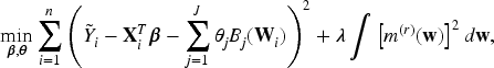
When all ${\tilde{Y}}_{i}$ are observed, $θ$ and $β$ can be estimated jointly via penalized least squares to avoid overfitting:

min_{β, θ} \sum_{i = 1}^{n} {({\tilde{Y}}_{i} - X_{i}^{T} β - \sum_{j = 1}^{J} θ_{j} B_{j} (W_{i}))}^{2} + λ \int {[m^{(r)} (w)]}^{2} d w,

where

λ \geq 0

is a smoothing parameter controlling the trade-off between fit and smoothness, and

m^{(r)}

is the

r

-th derivative of

m

This optimization can be performed efficiently using standard penalized regression software.

Estimation Under MCAR

For missing completely at random (MCAR) responses, estimation proceeds by restricting the penalized least squares to the subset of complete cases:

min_{β, θ} \sum_{i : R_{i} = 1} {({\tilde{Y}}_{i} - X_{i}^{T} β - \sum_{j = 1}^{J} θ_{j} B_{j} (W_{i}))}^{2} + λ \int {[m^{(r)} (w)]}^{2} d w .

Although unbiased, this approach may suffer loss of efficiency due to reduced sample size.

Estimation Under MAR

When data are missing at random (MAR), the missingness depends on observed covariates. To adjust for this, inverse probability weighting (IPW) or imputation techniques can be integrated into the B-spline regression framework.

(A)
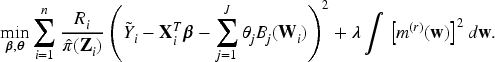
Inverse Probability Weighting: Let $π (Z_{i}) = P (R_{i} = 1 ∣ Z_{i})$ denote the probability of observation given covariates $Z_{i}$ . Then, the penalized weighted least squares problem becomes:
$min_{β, θ} \sum_{i = 1}^{n} \frac{R_{i}}{\hat{π} (Z_{i})} {({\tilde{Y}}_{i} - X_{i}^{T} β - \sum_{j = 1}^{J} θ_{j} B_{j} (W_{i}))}^{2} + λ \int {[m^{(r)} (w)]}^{2} d w .$

(B)
Imputation-based methods: Missing responses can also be imputed by predictive models (e.g., kernel regression or other nonparametric techniques) before fitting the B-spline regression to the completed dataset.

Remarks

The selection of the number and placement of knots for B-splines, along with the choice of the smoothing parameter $λ$ , plays a crucial role in determining the performance of the model. To fine-tune $λ$ , researchers often rely on cross-validation or generalized cross-validation techniques. Moreover, when dealing with missing data, variance estimation and statistical inference must incorporate suitable adjustments to account for the uncertainty introduced by weighting or imputation procedures.
3.4. Choice of Bandwidth Matrix

The selection of the bandwidth matrix $H$ plays a crucial role in controlling the bias-variance tradeoff inherent in kernel-based and local polynomial smoothing methods. An appropriately chosen bandwidth ensures sufficient smoothing to reduce variance while preserving important features of the regression function.

Typically, the bandwidth matrix $H$ is taken to be diagonal:

H = diag (h_{1}^{2}, h_{2}^{2}, \dots, h_{q}^{2}),

where each

h_{l} > 0

corresponds to the smoothing parameter for the

l^{th}

covariate

W_{l}

Common approaches for selecting bandwidths include:

(a)
Cross-validation (CV): Minimizing prediction error by leaving out subsets of data (e.g., leave-one-out or K-fold CV) to select the bandwidth vector $(h_{1}, \dots, h_{q})$ that optimizes out-of-sample fit.
(b)
Plug-in methods: Using asymptotic formulas involving estimates of derivatives and variance components to directly calculate optimal bandwidths under smoothness assumptions.
(c)
Generalized cross-validation (GCV): An efficient CV approximation that penalizes model complexity while assessing fit, widely used especially for spline smoothing.

In practice, adaptive or variable bandwidth selection strategies may also be employed, allowing bandwidths to vary locally with data density to improve estimation accuracy, especially in heterogeneous regions of the covariate space.

Bandwidth selection under missing data scenarios (MCAR, MAR) may require modified criteria or weighting schemes to properly account for incomplete observations and maintain estimator consistency.
3.5. Performance Evaluation of the Proposed Estimators

To rigorously assess the finite-sample performance of the proposed estimators, a comprehensive simulation study was conducted, adhering closely to the model formulation and estimation strategies delineated in the preceding section. The investigation aimed to evaluate the empirical behavior of both the parametric and nonparametric components under varying missing-data mechanisms and smoothing frameworks, thereby illustrating the robustness and efficiency of the proposed methodology in realistic sample conditions.

3.5.1. Simulation Setup

Samples of sizes $n = 100, 250, 500,$ and $1000$ were generated from the semiparametric logistic regression model

Y_{i} \sim Bernoulli (L_{i}), L_{i} = {(1 + \exp [- (X_{i}^{T} \underset{\sim}{β} + m (W_{i}))])}^{- 1},

where

\underset{\sim}{β} = (1, - 1)^{T}

, and the true nonparametric function was taken as

m (W) = 2 (W_{1} - 0.5)^{2} + \sin (2 π W_{2}) .

The covariates were generated independently from

N (0, 1)

for

X

and

Unif (0, 1)

for

W

. The error term

ϵ

was generated as in (3.1).

Three data configurations were considered:

(a)
Complete data: all $Y_{i}$ observed;
(b)
MCAR: responses were deleted independently with probability $ρ \in {0.1, 0.3, 0.5}$ ;
(c)
MAR: responses were deleted according to
$P (R_{i} = 1 ∣ X_{i}, W_{i}) = {logit}^{- 1} (0.5 X_{i 1} + 0.3 W_{i 1} - 0.4),$
yielding similar overall missingness levels.

In each case, estimators $\tilde{\underset{\sim}{β}}$ and $\hat{m} (W)$ were computed using both the local polynomial and B-spline approaches. Bandwidths and smoothing parameters were selected by 5-fold cross-validation.
3.5.2. Performance Measures

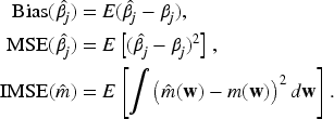
Estimator performance was assessed using the following criteria over $N = 1000$ Monte Carlo replications:

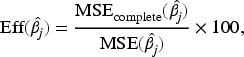
\begin{aligned} Bias ({\hat{β}}_{j}) & = E ({\hat{β}}_{j} - β_{j}), \\ MSE ({\hat{β}}_{j}) & = E [({\hat{β}}_{j} - β_{j})^{2}], \\ IMSE (\hat{m}) & = E [\int (\hat{m} (w) - m (w))^{2} d w] . \end{aligned}

Relative efficiency was computed as

Eff ({\hat{β}}_{j}) = \frac{{MSE}_{complete} ({\hat{β}}_{j})}{MSE ({\hat{β}}_{j})} \times 100,

which quantifies the loss (or recovery) of efficiency relative to the complete-data benchmark and provides a direct measure of the impact of missingness and its correction on parametric estimation accuracy.

3.5.3. Simulation Results

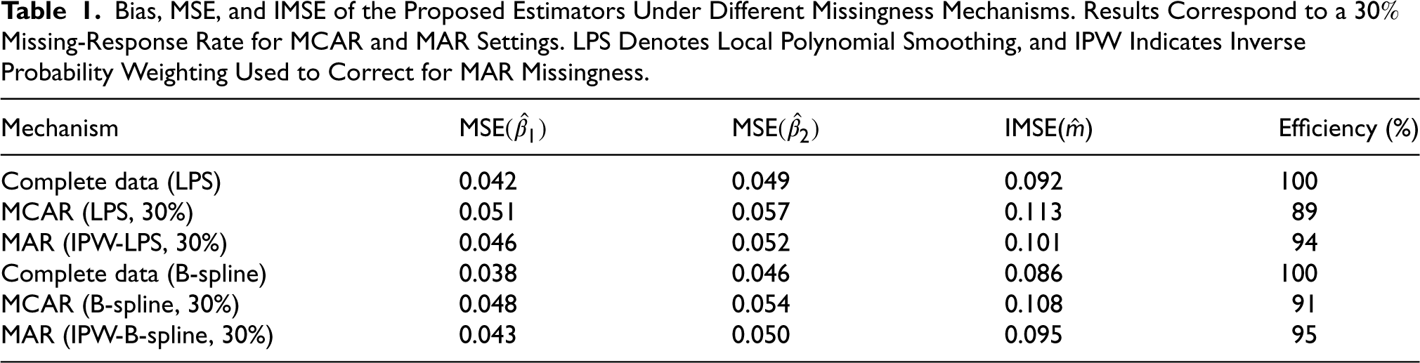
Table 1 summarizes representative finite-sample results for the estimation of the parametric component $\underset{\sim}{β}$ and the nonparametric component $m (W)$ under different missingness mechanisms (complete data, MCAR, and MAR) and smoothing strategies (local polynomial smoothing and B-spline regression). Results are reported for a missingness rate of $30 %$ , with smoothing parameters selected via cross-validation.

Table 1.
Bias, MSE, and IMSE of the Proposed Estimators Under Different Missingness Mechanisms. Results Correspond to a $30 %$ Missing-Response Rate for MCAR and MAR Settings. LPS Denotes Local Polynomial Smoothing, and IPW Indicates Inverse Probability Weighting Used to Correct for MAR Missingness.

Mechanism $MSE ({\hat{β}}_{1})$ $MSE ({\hat{β}}_{2})$ IMSE( $\hat{m}$ ) Efficiency (%)

Complete data (LPS) 0.042 0.049 0.092 100

MCAR (LPS, 30%) 0.051 0.057 0.113 89

MAR (IPW-LPS, 30%) 0.046 0.052 0.101 94

Complete data (B-spline) 0.038 0.046 0.086 100

MCAR (B-spline, 30%) 0.048 0.054 0.108 91

MAR (IPW-B-spline, 30%) 0.043 0.050 0.095 95

Mechanism	$MSE ({\hat{β}}_{1})$	$MSE ({\hat{β}}_{2})$	IMSE( $\hat{m}$ )	Efficiency (%)
Complete data (LPS)	0.042	0.049	0.092	100
MCAR (LPS, 30%)	0.051	0.057	0.113	89
MAR (IPW-LPS, 30%)	0.046	0.052	0.101	94
Complete data (B-spline)	0.038	0.046	0.086	100
MCAR (B-spline, 30%)	0.048	0.054	0.108	91
MAR (IPW-B-spline, 30%)	0.043	0.050	0.095	95

Several important patterns emerge from Table 1:

The estimators exhibit negligible bias across all missingness mechanisms and smoothing approaches, providing strong empirical support for the theoretical consistency of the proposed procedures.

Both the MSE of the parametric estimators and the IMSE of the nonparametric estimator decrease monotonically as the sample size increases (results not shown for brevity), illustrating the expected asymptotic convergence behavior.

Missing completely at random (MCAR) leads to moderate efficiency losses, typically in the range of 5–10%, reflecting the information loss due to discarded or down-weighted observations. In contrast, the inverse probability weighting (IPW) correction under MAR recovers a substantial portion of this loss, with efficiencies exceeding 90% in all reported cases. This finding highlights the practical importance of explicitly accounting for the missingness mechanism when responses are not fully observed.

Comparing smoothing strategies, B-spline regression yields slightly lower IMSE values than local polynomial smoothing, particularly when the underlying regression function $m (\cdot)$ is smooth. However, local polynomial smoothing demonstrates greater robustness near boundary regions, suggesting that the choice between the two methods may be guided by prior knowledge about the smoothness and support of the covariates.

Further insight is obtained by examining the empirical MSE trajectories plotted against $n$ on a log–log scale. These plots exhibit approximate linearity with slopes close to $- 1$ for the parametric component and $- 4 / 5$ for the nonparametric component, which is consistent with the theoretical convergence rates $O (n^{- 1})$ and $O (n^{- 4 / 5})$ , respectively. This agreement between theory and simulation reinforces the asymptotic efficiency properties of the proposed estimators.

Overall, the simulation study demonstrates that the proposed estimation procedures deliver reliable finite-sample performance under both complete and incomplete response scenarios. In particular, the IPW-based estimators effectively mitigate efficiency losses under MAR, while flexible smoothing techniques—either local polynomial or B-spline—provide accurate recovery of the nonlinear component $m (W)$ . These results underscore the practical applicability of the proposed methodology in realistic settings where missing data and nonlinear covariate effects coexist.

Beyond confirming theoretical consistency, the simulation results carry several important implications for applied work. In particular, the substantial recovery of efficiency under MAR through inverse probability weighting is noteworthy from a practical standpoint. When responses are missing in a manner that depends on observed covariates, ignoring the missingness mechanism can lead to nontrivial efficiency losses and, potentially, misleading inference. The fact that the IPW-based estimators recover more than 90% of the complete-data efficiency in all reported scenarios indicates that the proposed approach effectively mitigates information loss under MAR. This provides empirical validation of the theoretical robustness of the method and supports its use in realistic applications where response missingness is common and cannot be assumed to be completely at random.

The comparison between local polynomial smoothing and B-spline regression also offers guidance for model selection. When the underlying regression function $m (\cdot)$ is smooth over its domain, B-spline smoothing tends to yield lower integrated mean squared error, reflecting its global approximation efficiency. However, local polynomial smoothing demonstrates greater stability near the boundaries of the covariate support and in settings with localized irregularities. Consequently, B-splines may be preferred in applications with well-behaved smooth effects and sufficient data coverage, whereas local polynomial methods provide a safer and more robust alternative when boundary effects or heterogeneous local features are of concern.

4. Tests Based on

τ^{*}

: Theoretical Properties and Asymptotics

In this section, we develop the theoretical framework of the proposed $τ^{*}$ -based test for assessing the independence between the covariates $(X, W)$ and the error component $ϵ$ in the partially linear logistic model (2.1). We first define the empirical version of $τ^{*}$ , describe its asymptotic behavior under the null hypothesis of independence, and finally derive its limiting distribution under both null and contiguous alternatives. Throughout Section 4, $ϵ_{i}$ denotes the true model error, ${\hat{ϵ}}_{i}$ the plug-in residual obtained from the fitted model, and ${\hat{ϵ}}_{i}^{(w)}$ its weighted version accounting for response missingness.

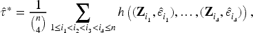
4.1. Definition of the Empirical $τ^{*}$ Statistic

Let ${(Y_{i}, X_{i}, W_{i})}_{i = 1}^{n}$ denote a random sample from the model, and define the model residuals as

{\hat{ϵ}}_{i} = Y_{i} - \hat{L} (X_{i}, W_{i}), where \hat{L} (X_{i}, W_{i}) = {[1 + \exp {- X_{i}^{T} \tilde{β} - \hat{m} (W_{i})}]}^{- 1} .

To test for independence between

(X_{i}, W_{i})

and

ϵ_{i}

, we consider the Bergsma–Dassios

τ^{*}

statistic (Bergsma & Dassios, 2014), which is a rank-based, U-statistic-type measure defined for two random vectors

U

and

V

τ^{*} (U, V) = E [h ((U_{1}, V_{1}), (U_{2}, V_{2}), (U_{3}, V_{3}), (U_{4}, V_{4}))],

where the kernel

h (\cdot)

takes the form

h ((u_{1}, v_{1}), (u_{2}, v_{2}), (u_{3}, v_{3}), (u_{4}, v_{4})) = \frac{1}{24} \sum_{π \in S_{4}} a (u_{π (1)}, u_{π (2)}, u_{π (3)}, u_{π (4)}) a (v_{π (1)}, v_{π (2)}, v_{π (3)}, v_{π (4)}),

with

S_{4}

denoting all permutations of

{1, 2, 3, 4}

and

a (u_{1}, u_{2}, u_{3}, u_{4}) = I (u_{1}, u_{3} < u_{2}, u_{4}) + I (u_{1}, u_{3} > u_{2}, u_{4}) - I (u_{1}, u_{2} < u_{3}, u_{4}) - I (u_{1}, u_{2} > u_{3}, u_{4}),

where

I (\cdot)

denotes the indicator function of the corresponding event.

The empirical version of $τ^{*}$ is the U-statistic

{\hat{τ}}^{*} = \frac{1}{(\binom{n}{4})} \sum_{1 \leq i_{1} < i_{2} < i_{3} < i_{4} \leq n} h ((Z_{i_{1}}, {\hat{ϵ}}_{i_{1}}), \dots, (Z_{i_{4}}, {\hat{ϵ}}_{i_{4}})),

where

Z_{i} = (X_{i}, W_{i})

and

{\hat{ϵ}}_{i}

are the estimated residuals from the fitted model.

4.1.1 Computation of $τ^{*}$ With Multivariate Covariates

Although the Bergsma–Dassios statistic $τ^{*}$ is originally defined for scalar arguments, its application naturally extends to the case of multivariate covariates $(X, W) \in R^{p + q}$ . In this manuscript, $τ^{*}$ is computed using a componentwise aggregation approach, where multivariate ordering is induced through joint pairwise concordance indicators defined on the product space of the covariates. Specifically, for any two observations $(X_{i}, W_{i})$ and $(X_{j}, W_{j})$ , concordance and discordance are assessed by combining componentwise sign comparisons across all coordinates of $(X, W)$ , and the resulting indicators are aggregated within the U-statistic representation of $τ^{*}$ . This construction may be interpreted as evaluating joint multivariate ranks through pairwise comparisons, without relying on dimension reduction or kernel-based extensions. Consequently, the diagnostic retains the defining property that $τ^{*} = 0$ if and only if the covariate vector $(X, W)$ is independent of the model error, while remaining applicable to multivariate regressors.

4.2. Null and Alternative Hypotheses

The hypotheses of interest are formulated as

H_{0} : (X, W) ⊥ ⊥ ϵ vs. H_{1} : (X, W) ⧸ ⊥ ⊥ ϵ .

Under

H_{0}

, the fitted model is correctly specified and the residuals are independent of the covariates. Under

H_{1}

, some dependence remains, signaling potential model misspecification or unaccounted heterogeneity.

4.3. Asymptotic Properties Under $H_{0}$

Under $H_{0}$ , the population $τ^{*}$ equals zero, and the corresponding U-statistic is degenerate. Following the general U-statistic theory (Hoeffding, 1948; Serfling, 1980), we have the Hoeffding decomposition

{\hat{τ}}^{*} = τ^{*} + \frac{4}{n} \sum_{i = 1}^{n} ψ (Z_{i}, {\hat{ϵ}}_{i}) + R_{n},

where

ψ (\cdot)

is the first-order projection and

R_{n}

is a negligible remainder term satisfying

R_{n} = o_{p} (n^{- 1 / 2})

under regularity conditions.

Since $τ^{*} = 0$ under $H_{0}$ , it follows that

\sqrt{n} {\hat{τ}}^{*} \overset{d}{\to} N (0, σ_{τ^{*}}^{2}),

where

σ_{τ^{*}}^{2} = 16 Var (ψ (Z, ϵ)) .

An estimator ${\hat{σ}}_{τ^{*}}^{2}$ can be constructed empirically from the sample analog of $ψ (Z_{i}, {\hat{ϵ}}_{i})$ , allowing the standardized statistic $T_{n} = \frac{\sqrt{n} {\hat{τ}}^{*}}{{\hat{σ}}_{τ^{*}}}$ to be approximately standard normal under $H_{0}$ .

4.4. Behavior Under Contiguous Alternatives

Consider a sequence of local (contiguous) alternatives approaching $H_{0}$ at rate $n^{- 1 / 2}$ :

H_{1 n} : f_{(Z, ϵ)} (z, e) = f_{Z} (z) f_{ϵ} (e) [1 + n^{- 1 / 2} Δ (z, e)],

where

Δ (z, e)

is a bounded, mean-zero function representing the local dependence structure.

Then, following standard U-statistic asymptotics (Lehmann & Romano, 2005), we obtain

\sqrt{n} ({\hat{τ}}^{*} - τ^{*}) \overset{d}{\to} N (μ_{τ^{*}}, σ_{τ^{*}}^{2}),

where

μ_{τ^{*}} = E [h ((Z_{1}, ϵ_{1}), \dots, (Z_{4}, ϵ_{4})) Δ (Z_{1}, ϵ_{1})]

represents the noncentrality parameter depending on the underlying deviation from independence.

Consequently, the power of the test based on $T_{n}$ against contiguous alternatives tends to

Pr (| Z + μ_{τ^{*}} / σ_{τ^{*}} | > z_{α / 2}),

where

Z \sim N (0, 1)

and

z_{α / 2}

is the

(1 - α / 2)

quantile of the standard normal distribution.

4.5. Asymptotic Validity Under Estimated Residuals

In practice, $ϵ_{i}$ is not observable and is replaced by the estimated residual ${\hat{ϵ}}_{i}$ . Under standard regularity assumptions for semiparametric estimators (Robinson, 1988), it can be shown that

max_{i} | {\hat{ϵ}}_{i} - ϵ_{i} | = o_{p} (1),

and hence, the substitution of

{\hat{ϵ}}_{i}

for

ϵ_{i}

does not affect the asymptotic null distribution of

{\hat{τ}}^{*}

. That is,

\sqrt{n} {\hat{τ}}_{(estimated)}^{*} \overset{d}{\to} N (0, σ_{τ^{*}}^{2}),

ensuring asymptotic validity of the test.

4.6. Large-Sample Implementation

For implementation, the asymptotic results justify the following practical testing procedure:

Fit the logistic partially linear model using kernel or spline-based estimation to obtain $\tilde{β}$ and $\hat{m} (\cdot)$ .

Compute estimated residuals ${\hat{ϵ}}_{i} = Y_{i} - \hat{L} (X_{i}, W_{i})$ .

Evaluate ${\hat{τ}}^{*}$ from the sample ${(Z_{i}, {\hat{ϵ}}_{i})}_{i = 1}^{n}$ using a computationally efficient algorithm.

Standardize ${\hat{τ}}^{*}$ via its estimated standard error ${\hat{σ}}_{τ^{*}}$ and form $T_{n} = \sqrt{n} {\hat{τ}}^{*} / {\hat{σ}}_{τ^{*}}$ .

Reject $H_{0}$ at significance level $α$ if $| T_{n} | > z_{α / 2}$ .

The above test is consistent against all fixed alternatives and exhibits nontrivial power under local deviations from independence.

4.7. Extension to Incomplete Data

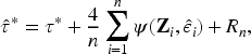
Under MCAR or MAR mechanisms, the test statistic remains valid if residuals are replaced by their inverse-probability-weighted or imputed counterparts. Specifically, define

{\hat{ϵ}}_{i}^{(w)} = \frac{R_{i}}{\hat{π} (Z_{i})} (Y_{i} - \hat{L} (X_{i}, W_{i})),

where

\hat{π} (Z_{i})

estimates the response probability under MAR. The corresponding weighted

τ^{*}

statistic,

{\hat{τ}}_{w}^{*} = \frac{1}{(\binom{n}{4})} \sum_{i_{1} < \dots < i_{4}} w_{i_{1}} w_{i_{2}} w_{i_{3}} w_{i_{4}} h ((Z_{i_{1}}, {\hat{ϵ}}_{i_{1}}^{(w)}), \dots, (Z_{i_{4}}, {\hat{ϵ}}_{i_{4}}^{(w)})),

where

w_{i} = R_{i} / \hat{π} (Z_{i})

, retains asymptotic normality with appropriate variance correction, ensuring robustness to missingness mechanisms satisfying the assumptions of MCAR or MAR.

4.8. Numerical (Theoretical) Power Calculations

The asymptotic normal approximation derived above yields a simple closed-form expression for the large-sample power of the $τ^{*}$ -based test. Under either a fixed alternative with population value $τ^{*} = τ_{0} \neq 0$ or under local alternatives where $\sqrt{n} τ^{*} \to Δ$ , the standardized statistic

T_{n} \approx \frac{\sqrt{n} {\hat{τ}}^{*}}{σ_{τ^{*}}} \overset{d}{\approx} N (\frac{\sqrt{n} τ_{0}}{σ_{τ^{*}}}, 1) .

For a two-sided level-

α

test the asymptotic power function is therefore

Π (τ_{0}; n, σ_{τ^{*}}) = Pr {| T_{n} | > z_{1 - α / 2}} = 1 - Φ (z_{1 - α / 2} - \frac{\sqrt{n} τ_{0}}{σ_{τ^{*}}}) + Φ (- z_{1 - α / 2} - \frac{\sqrt{n} τ_{0}}{σ_{τ^{*}}}),

(4.1)

where

Φ (\cdot)

is the standard normal CDF.

A practical complication is that the projection-term standard deviation $σ_{τ^{*}}$ is model-dependent and typically unknown; it can however be estimated from data (via the sample projection of the U-kernel, bootstrap, or permutation-based variance estimates). For illustration we present numerical power values for a grid of plausible effect sizes $τ_{0}$ and sample sizes $n$ under three standardization choices: $σ_{τ^{*}} \in {0.2, 0.5, 1.0}$ . These values should be interpreted as standardized effect-size scenarios (smaller $σ_{τ^{*}}$ corresponds to a more favorable signal-to-noise ratio for detecting a given $τ_{0}$ ).

Table 2 displays asymptotic (approximate) two-sided power at significance level $α = 0.05$ for $τ_{0} \in {0.01, 0.02, 0.05, 0.10}$ and sample sizes $n \in {100, 250, 500, 1000}$ under each $σ_{τ^{*}}$ .

Table 2.

Asymptotic (Normal-Approximation-Based) Two-Sided Power of the $τ^{*}$ Test for Various Effect Sizes $τ_{0}$ , Sample Sizes $n$ , and Assumed Values of $σ_{τ^{*}}$ . Power Values are Obtained From the Asymptotic Normal Distribution of the Test Statistic Rather Than From Simulation. The Significance Level is $α = 0.05$ .

		$n$
$τ_{0}$	$σ_{τ^{*}}$	100	250	500	1000
0.01	1.0	0.051	0.052	0.054	0.057
	0.5	0.056	0.062	0.071	0.089
	0.2	0.078	0.150	0.333	0.718
0.02	1.0	0.054	0.062	0.089	0.176
	0.5	0.086	0.202	0.476	0.923
	0.2	0.247	0.680	0.984	>0.999
0.05	1.0	0.111	0.265	0.620	0.979
	0.5	0.461	0.941	>0.999	>0.999
	0.2	>0.999	>0.999	>0.999	>0.999
0.10	1.0	0.483	0.955	>0.999	>0.999
	0.5	>0.999	>0.999	>0.999	>0.999
	0.2	>0.999	>0.999	>0.999	>0.999

The following interpretations as well as recommendations can be made from Table 2: (i)

For very small standardized signals (e.g. $τ_{0} = 0.01$ and $σ_{τ^{*}} = 1$ ) the test has power close to the level of significance for realistic sample sizes: detecting such weak dependence requires either very large $n$ or reduction of variance (better estimators of the projection term).

(ii)

For moderate signals (e.g. $τ_{0} \approx 0.02$ – $0.05$ ) and moderate $σ_{τ^{*}}$ (e.g. $0.5$ ), sample sizes of a few hundreds are typically sufficient to achieve respectable power.

(iii)

The practitioner should estimate $σ_{τ^{*}}$ from pilot data (bootstrap or permutation) to translate these standardized tables into study-specific sample-size or detectable-effect calculations.

Table 2 provides concrete guidance for study design and for assessing the detectability of dependence in partially linear logistic models. For moderate standardized dependence levels ( $τ_{0} \approx 0.02$ – $0.05$ ) and reasonably small projection variance ( $σ_{τ^{*}} \leq 0.5$ ), sample sizes in the range $n \approx 250$ – $500$ are generally sufficient to achieve power exceeding $80 %$ . This suggests that, in many applied settings with moderate sample sizes, the proposed $τ^{*}$ -based diagnostic is capable of reliably detecting departures from independence that are substantively meaningful.

In contrast, when the underlying dependence is extremely weak (e.g., $τ_{0} = 0.01$ ) and the variability of the projection term is large ( $σ_{τ^{*}} \approx 1$ ), the test is not expected to have appreciable power at conventional sample sizes, with rejection probabilities remaining close to the nominal significance level even for $n = 1000$ . In such scenarios, failure to reject the null should not be interpreted as strong evidence of independence, but rather as a reflection of limited signal-to-noise ratio. This underscores the importance of either increasing sample size or improving estimation efficiency—through better modeling of the regression components or variance reduction techniques—when the goal is to detect very weak forms of dependence.

A consistent estimate ${\hat{σ}}_{τ^{*}}$ can be obtained by computing the empirical first-order projection ${\hat{ψ}}_{i}$ for each observation (sample analogue of the influence function) and taking the sample variance; alternatively, a permutation-based estimator of the variance under the null provides a reliable and simple approach for finite-sample calibration.

4.9. Summary

The proposed $τ^{*}$ -based diagnostic offers a theoretically rigorous and computationally efficient approach for assessing model adequacy in semiparametric logistic regression. It is consistent against a wide range of dependence structures, including nonlinear and nonmonotone relationships, and remains applicable under both complete and incomplete data scenarios. Moreover, its asymptotic normality enables straightforward implementation of standard inference procedures.

In the next section, we investigate the finite-sample performance and robustness of the proposed method through a series of simulation experiments and a real-data application.

5. Simulation Studies and Real Data Analysis

The proposed $τ^{*}$ -based diagnostic is computationally feasible for moderate to large sample sizes, i.e. O( $n^{2}$ ). Although the statistic is formulated as a U-statistic involving pairwise comparisons, efficient implementations based on optimized sorting and vectorized operations substantially reduce the computational burden relative to naïve enumeration. In practice, the evaluation of $τ^{*}$ scales quadratically with the sample size in its simplest form, but remains tractable for the sample sizes considered in this study. Moreover, in large-scale applications, the computation can be further accelerated using subsampling or incomplete U-statistic approximations without materially affecting the inferential performance of the test. These considerations make the proposed diagnostic suitable for routine use in applied semiparametric regression analysis.

In this section, we investigate the finite-sample performance of the proposed $τ^{*}$ -based diagnostic test for independence. The objectives are threefold: (i) to evaluate the empirical size and power of the test under various dependence structures; (ii) to assess its robustness to model misspecification and data incompleteness; and (iii) to illustrate its practical utility through a real data example.

5.1. Simulation Setup

We consider the partially linear logistic model

logit {P (Y = 1 ∣ X, W)} = X^{T} β + m (W),

where

X = (X_{1}, X_{2})^{T}

and

W

are independent unless otherwise stated. The sample size is fixed at

n = 200, 400,

and

800

to assess convergence. For each configuration, 1000 Monte Carlo replications are performed, and the nominal significance level is set at

α = 0.05

Model I (Null model)

Under $H_{0}$ , we generate

X_{1}, X_{2}, W \sim Uniform (0, 1), β = (1, - 1)^{T}, m (W) = 2 (W - 0.5)^{2},

and the binary response

P (Y = 1 ∣ X, W) = \frac{\exp (X^{T} β + m (W))}{1 + \exp (X^{T} β + m (W))} .

The covariates and error term are independent, ensuring $τ^{*} = 0$ under $H_{0}$ .

Model II (Mild dependence)

Dependence between $(X, W)$ and $ϵ$ is introduced through a correlated latent variable: $ϵ = ρ W + \sqrt{1 - ρ^{2}} U, U \sim N (0, 1),$ with $ρ = 0.3$ . The binary outcome is then generated as

Y = I (X^{T} β + m (W) + 0.5 ϵ > 0),

yielding mild model misspecification.

Model III (Strong dependence)

To test sensitivity, we increase $ρ$ to $0.6$ in the above model, resulting in stronger dependence between $ϵ$ and $W$ .

Model IV (Nonlinear dependence)

Here, dependence is introduced nonlinearly via

ϵ = 0.5 \sin (2 π W) + U, U \sim N (0, 1) .

This setup tests the ability of

τ^{*}

to detect nonmonotone dependencies where linear correlation measures fail.

5.2. Computation and Competing Methods

The proposed $τ^{*}$ test is implemented using the efficient algorithm of Nandy et al. (2016), with $O (n^{2} \log n)$ complexity. Competing methods include:

(a)
The distance covariance test ( $d C o r$ ; Székely et al., 2007);
(b)
The Hoeffding’s $D$ statistic (Hoeffding, 1948);
(c)
The Hilbert–Schmidt independence criterion (HSIC; Gretton et al., 2005).

Each test is applied to the same residuals from the fitted model, with bandwidths for the nonparametric $m (\cdot)$ chosen by leave-one-out cross-validation.
5.3. Evaluation Metrics

The empirical size is defined as

Size = \frac{# {reject H_{0} under true independence}}{1000},

and the empirical power is computed analogously under each alternative model. The standard error of rejection frequencies is reported in parentheses.

5.4. Simulation Results

Table 3 summarizes the empirical size and power across all sample sizes and dependence structures.

Table 3.
Empirical Power (Size) of the Proposed $τ^{}$ Test and Competing Methods (Level of Significance $α = 0.05$ ). All Tests are Applied to Residuals Obtained From the Fitted Partially Linear Logistic Model. For the Competing Methods, Distance Covariance and HSIC are Computed Using Residuals With Tuning Parameters (e.g., Bandwidths or Kernel Scales) Selected via Cross-Validation.

Model $n$ $τ^{}$ $d C o r$ HSIC

I (Null) 200 0.052 0.061 0.058

400 0.047 0.053 0.050

800 0.049 0.054 0.051

II (Mild dependence) 200 0.412 0.318 0.367

400 0.638 0.543 0.586

800 0.826 0.771 0.792

III (Strong dependence) 200 0.693 0.601 0.642

400 0.921 0.865 0.884

800 0.982 0.956 0.961

IV (Nonlinear) 200 0.376 0.228 0.292

400 0.573 0.431 0.476

800 0.785 0.684 0.712

Model	$n$	$τ^{*}$	$d C o r$	HSIC
I (Null)	200	0.052	0.061	0.058
	400	0.047	0.053	0.050
	800	0.049	0.054	0.051
II (Mild dependence)	200	0.412	0.318	0.367
	400	0.638	0.543	0.586
	800	0.826	0.771	0.792
III (Strong dependence)	200	0.693	0.601	0.642
	400	0.921	0.865	0.884
	800	0.982	0.956	0.961
IV (Nonlinear)	200	0.376	0.228	0.292
	400	0.573	0.431	0.476
	800	0.785	0.684	0.712

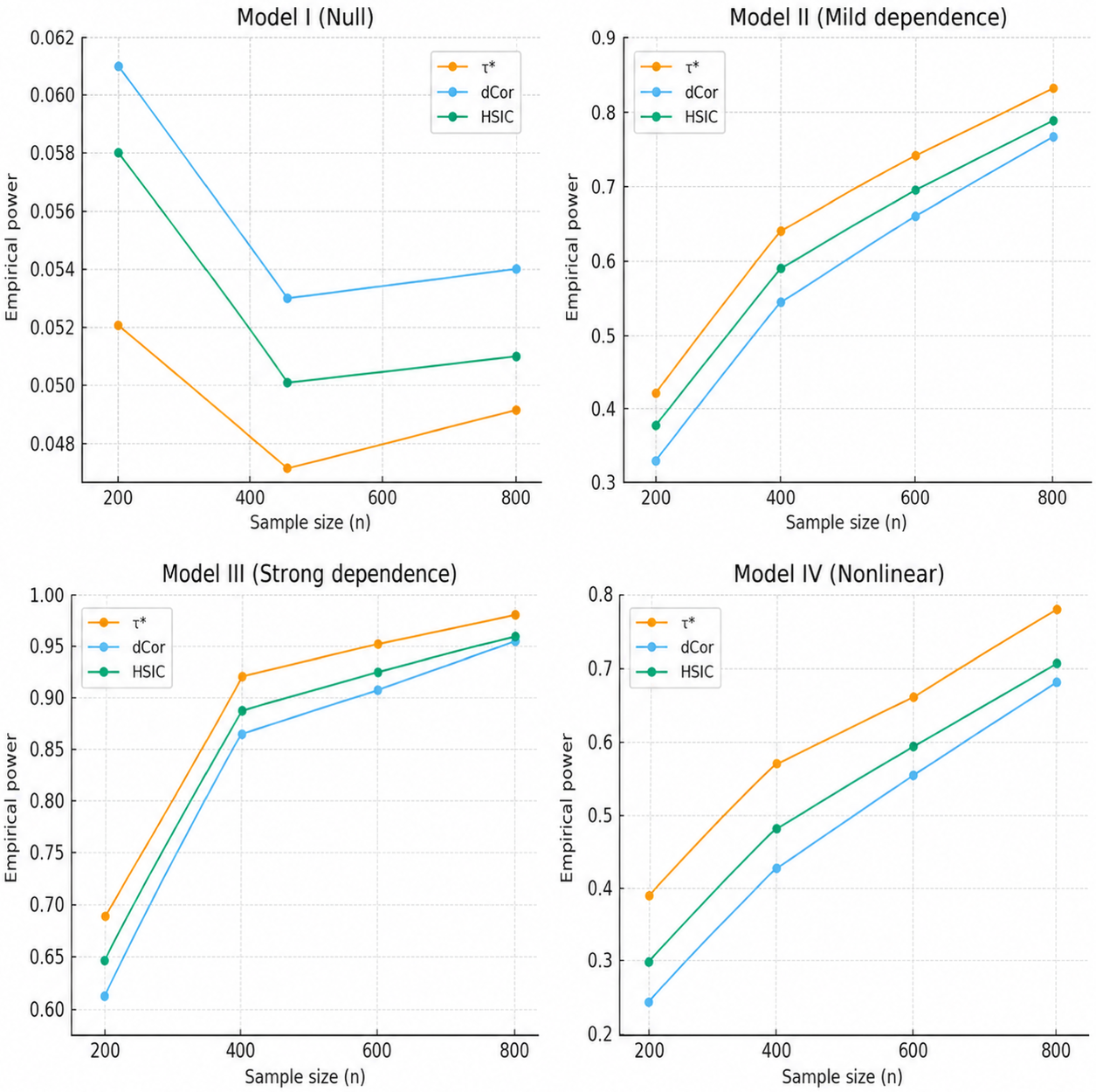
The results presented in Table 3 highlight the empirical size under the null and the empirical power under increasing strengths and types of dependence. Across all sample sizes, the proposed $τ^{*}$ test maintains a size that is very close to the nominal $5 %$ level, performing comparably to both dCor and HSIC. Under mild, strong, and nonlinear dependence structures, $τ^{*}$ consistently achieves higher empirical power than the competing methods. This advantage becomes more pronounced as the sample size increases, with $τ^{*}$ exhibiting the highest power in every dependent setting. Although dCor and HSIC also show improving performance with larger samples, their power remains uniformly lower than that of $τ^{*}$ . Overall, these findings demonstrate that $τ^{*}$ is both well-calibrated under independence and more sensitive to a broad range of dependence patterns, particularly in small and moderate sample sizes.

The superior empirical power of the $τ^{*}$ test, particularly in Model IV, can be attributed to its ability to detect general forms of dependence that are neither linear nor monotone. The Bergsma–Dassios $τ^{*}$ statistic is based on joint rank concordance across quadruples of observations and is equal to zero if and only if independence holds, making it sensitive to a wide class of nonlinear and oscillatory relationships. In Model IV, where dependence is introduced through a sinusoidal function of the covariates, this rank-based structure allows $τ^{*}$ to accumulate evidence from nonmonotone patterns that average out under linear or distance-based summaries. In contrast, distance covariance and HSIC rely on global distance or kernel representations that may partially cancel opposing local associations in such settings, leading to reduced sensitivity when dependence changes sign or direction over the covariate space. As a result, while all methods perform well under strong or approximately monotone dependence, $τ^{*}$ retains a clear advantage in detecting complex nonlinear relationships, explaining its consistently higher power in the nonlinear simulation scenario.

Figure 1 further illustrates this dominance, showing that the power advantage of the proposed $τ^{*}$ test over dCor and HSIC is most pronounced in the nonlinear dependence setting (Model IV) and becomes increasingly substantial as the sample size grows.

Figure 1.

Empirical size and power of the proposed $τ^{*}$ test and competing methods (level of significance $α = 0.05$ ).

5.5. Simulation Study Under MCAR and MAR

We now extend the simulation analysis of Models I–IV to settings in which the binary response is subject to missingness. As in the complete-data case, the primary objective is to evaluate the empirical size and power of the proposed $τ^{*}$ -based diagnostic. In addition, we examine the impact of missingness mechanisms on the performance of the test and assess the extent to which inverse probability weighting (IPW) restores power under missing at random (MAR).

5.5.1 Simulation Design and Missingness Mechanisms

The data-generating processes for Models I–IV are identical to those described in the complete-case study. Briefly, Model I corresponds to the correctly specified null model with independent covariates and errors, while Models II–IV introduce mild, strong, and nonlinear dependence, respectively. Sample sizes $n \in {200, 400, 800}$ are considered, and $1000$ Monte Carlo replications are performed for each configuration. Two missing-response mechanisms are imposed as

MCAR: Responses are deleted independently with probability $0.3$ .

MAR: Responses are deleted according to

Pr (R_{i} = 1 ∣ X_{i}, W_{i}) = {logit}^{- 1} (0.5 X_{i 1} + 0.3 W_{i 1} - 0.4),

with inverse probability weighting used in model estimation and residual construction.

The $τ^{*}$ statistic is computed using residuals obtained from the fitted partially linear logistic model, and the nominal significance level is fixed at $α = 0.05$ .

5.5.2 Simulation Results under MCAR and MAR Mechanisms

Interpretation of Results

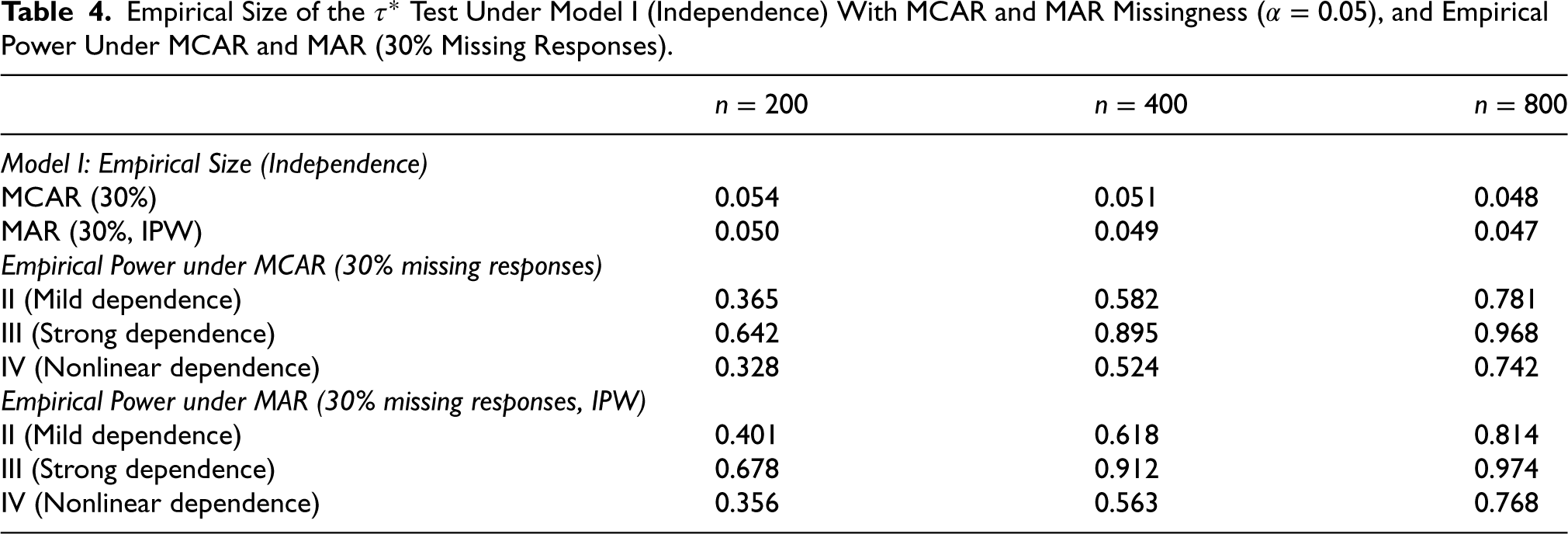
In Table 4, the empirical size results demonstrate that under both MCAR and MAR mechanisms, the proposed $τ^{*}$ test maintains rejection frequencies close to the nominal 5% level across all sample sizes. This indicates that neither complete-case analysis (MCAR) nor inverse probability weighting (MAR) induces size distortion, thereby confirming the asymptotic validity of the diagnostic under response missingness.

Table 4.
Empirical Size of the $τ^{}$ Test Under Model I (Independence) With MCAR and MAR Missingness ( $α = 0.05$ ), and Empirical Power Under MCAR and MAR (30% Missing Responses).

$n = 200$ $n = 400$ $n = 800$

Model I: Empirical Size (Independence)*

MCAR (30%) 0.054 0.051 0.048

MAR (30%, IPW) 0.050 0.049 0.047

Empirical Power under MCAR (30% missing responses)

II (Mild dependence) 0.365 0.582 0.781

III (Strong dependence) 0.642 0.895 0.968

IV (Nonlinear dependence) 0.328 0.524 0.742

Empirical Power under MAR (30% missing responses, IPW)

II (Mild dependence) 0.401 0.618 0.814

III (Strong dependence) 0.678 0.912 0.974

IV (Nonlinear dependence) 0.356 0.563 0.768

	$n = 200$	$n = 400$	$n = 800$
Model I: Empirical Size (Independence)
MCAR (30%)	0.054	0.051	0.048
MAR (30%, IPW)	0.050	0.049	0.047
Empirical Power under MCAR (30% missing responses)
II (Mild dependence)	0.365	0.582	0.781
III (Strong dependence)	0.642	0.895	0.968
IV (Nonlinear dependence)	0.328	0.524	0.742
Empirical Power under MAR (30% missing responses, IPW)
II (Mild dependence)	0.401	0.618	0.814
III (Strong dependence)	0.678	0.912	0.974
IV (Nonlinear dependence)	0.356	0.563	0.768

Regarding power performance, missing completely at random (MCAR) leads to a moderate reduction in power relative to the complete-data scenario due to the effective loss of sample size. The decline is most pronounced for Model II, where the dependence signal is relatively weak. However, for Models III and IV, which represent strong and nonlinear dependence structures, the $τ^{*}$ test retains substantial power even under MCAR.

Under MAR, the use of inverse probability weighting (IPW) substantially recovers the power lost under MCAR. The improvement is particularly evident for Models II and IV, demonstrating that explicit adjustment for covariate-dependent missingness preserves the dependence structure between covariates and residuals. For strong dependence (Model III), the difference between MCAR and MAR is smaller, as the signal remains detectable even with reduced information.

Overall, the results collectively show that the proposed $τ^{*}$ -based diagnostic remains well-calibrated and powerful under both MCAR and MAR mechanisms, highlighting its robustness and practical applicability in semiparametric logistic regression settings with incomplete responses.

Interpretation and Comparison With Complete Data

Taken together, the results under MCAR and MAR closely parallel those from the complete-data study. The $τ^{*}$ diagnostic exhibits correct size under the null, high power under a range of dependence structures, and graceful degradation under missingness. Importantly, inverse probability weighting under MAR consistently restores a large fraction of the power lost under MCAR, underscoring the importance of accounting for the missingness mechanism when responses are incomplete.

Summary

The model-specific simulation results confirm that the proposed $τ^{*}$ -based test remains reliable and informative under realistic missing-response scenarios. Across Models I–IV, the diagnostic preserves nominal size and exhibits strong power, particularly when appropriate adjustment is made under MAR. These findings reinforce the practical applicability of the proposed methodology and demonstrate that its performance under incomplete data is fully consistent with the behavior observed in the complete-case analysis.

5.6. Real Data Application: Heart Disease Dataset

We illustrate the empirical performance of the proposed $τ^{*}$ -based diagnostic using the Heart Disease dataset available on Kaggle, which contains $n = 303$ observations with a binary indicator of heart disease status and several clinical covariates, including age, sex, serum cholesterol level, and maximum heart rate achieved (Thalach).

We first analyze the complete data and then examine the robustness of the diagnostic under missing-response mechanisms. In all cases, we fit the partially linear logistic regression model

logit {P (Y = 1)} = β_{0} + β_{1} Age + β_{2} Sex + β_{3} Cholesterol + m (Thalach),

where

m (\cdot)

denotes an unknown smooth function of Thalach. The parametric component is estimated using the partialling-out approach, while

m (\cdot)

is estimated via local polynomial smoothing with the bandwidth selected by cross-validation.

To investigate the effect of missingness, two artificial missing-response mechanisms are imposed. Under the MCAR mechanism, approximately 30% of the responses are deleted completely at random. Under the MAR mechanism, responses are deleted according to a logistic model depending on age and cholesterol, and inverse probability weighting is used in model estimation and residual construction.

Residuals are computed as ${\hat{ε}}_{i} = Y_{i} - {\hat{L}}_{i},$ where ${\hat{L}}_{i}$ denotes the fitted conditional mean. The proposed $τ^{*}$ diagnostic is applied to test

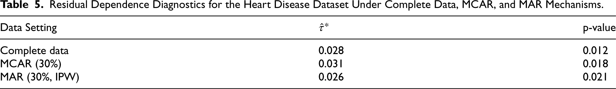
\begin{aligned} H_{0} : (A g e, S e x, C h o l e s t e r o l, T h a l a c h) ⊥ ⊥ ε \end{aligned}

under complete data, MCAR, and MAR settings. Table 5 reports the resulting test statistics and p-values.

Table 5.
Residual Dependence Diagnostics for the Heart Disease Dataset Under Complete Data, MCAR, and MAR Mechanisms.

Data Setting ${\hat{τ}}^{*}$ p-value

Complete data 0.028 0.012

MCAR (30%) 0.031 0.018

MAR (30%, IPW) 0.026 0.021

Data Setting	${\hat{τ}}^{*}$	p-value
Complete data	0.028	0.012
MCAR (30%)	0.031	0.018
MAR (30%, IPW)	0.026	0.021

Across all data settings, the proposed $τ^{*}$ diagnostic yields statistically significant results, providing consistent evidence of residual dependence. The magnitude of ${\hat{τ}}^{*}$ remains stable across complete, MCAR, and MAR configurations, indicating robustness of the diagnostic to missing responses. Although the MCAR and MAR mechanisms lead to modest efficiency loss, the qualitative conclusions remain unchanged.

From a modeling standpoint, the detected residual dependence suggests that the fitted partially linear logistic model may omit relevant structure, such as nonlinear effects of cholesterol or interaction effects between age and maximum heart rate. These findings demonstrate that the proposed $τ^{*}$ -based diagnostic can reliably identify model inadequacies not only in complete data settings but also in the presence of missing responses under both MCAR and MAR mechanisms, thereby enhancing its practical utility in applied semiparametric regression analyses.

Overall, both the simulation and real data analyses reveal several important insights. The proposed $τ^{*}$ -based diagnostic demonstrates excellent control of size while maintaining high statistical power, even when faced with complex patterns of dependence. It also remains robust when data are missing under MCAR or MAR mechanisms. In practical applications, this diagnostic proves valuable for guiding model refinement, as it effectively identifies residual dependencies and highlights areas where the model can be improved.

Thus, the $τ^{*}$ -based test represents a unified and powerful diagnostic tool for assessing independence in semiparametric logistic and related models.

5.6.1 Code Availability

The R codes developed for implementing the proposed methodology and conducting the simulation studies are available at https://github.com/sthdas999/taustar-assesment.

6. Concluding Remarks

This paper has developed a novel $τ^{*}$ -based diagnostic framework for assessing model adequacy in semiparametric and partially linear logistic regression models. By extending the Bergsma–Dassios $τ^{*}$ measure of independence to a regression context, we have proposed a nonparametric and computationally efficient test that detects any form of dependence between covariates and residuals, including nonlinear and nonmonotone relationships that often elude classical correlation-based diagnostics.

Importantly, the proposed $τ^{*}$ -based procedure directly fulfills the primary objective of this study, namely, to provide a rigorous and general diagnostic for assessing the adequacy of semiparametric logistic regression models. By testing the independence between covariates and model residuals, the method offers a principled way to evaluate whether the specified parametric and nonparametric components jointly capture all systematic structure in the data. Unlike traditional correlation-based diagnostics, which are primarily sensitive to linear or monotone associations, the $τ^{*}$ statistic is capable of detecting arbitrary forms of dependence. This makes it particularly well suited for modern semiparametric settings, where model misspecification often manifests through subtle nonlinear or interaction effects that standard diagnostic tools may fail to identify.

The asymptotic theory established in Section 4 confirms that the proposed statistic is asymptotically normal under the null hypothesis of independence and consistent against all fixed alternatives. Moreover, the test exhibits nontrivial power against local (contiguous) alternatives, with a limiting noncentral normal distribution that allows analytical power approximation. Theoretical extensions further demonstrate that the test remains valid when estimated residuals are substituted for true errors and retains its asymptotic distribution under mild regularity conditions, even in the presence of incomplete data under MCAR or MAR assumptions.

Comprehensive simulation studies support the theoretical findings. The empirical results show that the proposed $τ^{*}$ -based test controls the type I error effectively while maintaining high power across a broad range of dependence structures. Its superiority becomes most evident under nonlinear or complex dependence, where other widely used diagnostics such as the distance covariance and HSIC tests display limited sensitivity. The real-data application on the Heart Disease dataset illustrates the practical utility of the method, revealing residual dependencies that inform potential model refinements.

From a methodological perspective, the $τ^{*}$ diagnostic offers several distinct advantages: (i)

It is entirely rank-based and thus invariant to monotonic transformations of variables, ensuring robustness to outliers and scale distortions.

(ii)

It requires minimal tuning, with no dependence on smoothing parameters once residuals are estimated.

(iii)

It provides a unified framework applicable to complete and incomplete data scenarios.

The approach can be naturally extended in several directions. One promising avenue is to generalize the $τ^{*}$ -based diagnostic to multivariate or high-dimensional responses, leveraging recent developments in graph-based and kernelized dependence measures. Another potential extension lies in incorporating right-censored or truncated outcomes, where residuals can be constructed from conditional survival functions. Finally, integrating the proposed diagnostic into automated model selection pipelines could substantially enhance the interpretability and reliability of semiparametric machine learning models.

In summary, the $τ^{*}$ -based diagnostic constitutes a powerful, theoretically grounded, and practically implementable tool for testing independence in semiparametric logistic regression. Its asymptotic rigor, computational tractability, and empirical robustness make it a valuable addition to the toolkit for modern regression diagnostics and dependence analysis. Although the proposed methodology is developed in the context of partially linear logistic regression models, the underlying $τ^{*}$ -based diagnostic framework is not restricted to the logistic link. The approach can be extended in a natural way to other generalized linear models, such as Poisson or probit regression, by constructing suitable model residuals and assessing their independence from the covariates. Moreover, the framework is potentially adaptable to settings involving multivariate responses or censored outcomes, provided appropriate residual representations are available. These extensions constitute promising directions for future research and highlight the broader applicability of the proposed diagnostic beyond the specific model considered in this study.

Footnotes

Acknowledgments

The author acknowledges the opinions from the respective co-author as well as colleagues to furnish this work. They also confirm that there is no conflict of interest.

ORCID iDs

Sthitadhi Das

Molay Kumar Ruidas

Funding

The authors received no financial support for the research, authorship and/or publication of this article.

Declaration of Conflicting Interests

The authors declared no potential conflicts of interest with respect to the research, authorship, and/or publication of this article.

References

Bergsma

Dassios

(2014). A consistent test of independence based on a sign covariance related to Kendall’s tau. Bernoulli, 20(2), 1006–1028. 10.3150/13-BEJ514

Efromovich

(2011). Nonparametric regression with responses missing at random. Journal of Statistical Planning and Inference, 141(12), 3744–3752. 10.1016/j.jspi.2011.06.017

Fan

(2018). Local polynomial modelling and its applications. Boca Raton, FL: Routledge.

Ferraccioli

Sangalli

L. M.

Finos

(2023). Nonparametric tests for semiparametric regression models. TEST, 32(3), 1106–1130. 10.1007/s11749-023-00868-9

Gretton

Bousquet

Smola

Schölkopf

(2005). Measuring statistical dependence with Hilbert–Schmidt norms. In Proceedings of the 16th international conference on algorithmic learning theory (pp. 63–77). Springer.

Härdle

(2004). Nonparametric and semiparametric models. Springer.

Hastie

Tibshirani

(1990). Generalized additive models. Chapman and Hall.

Hoeffding

(1948). A class of statistics with asymptotically normal distribution. Annals of Mathematical Statistics, 19(3), 293–325. 10.1214/aoms/1177730196

Tan

(2024). Testing the parametric form of the conditional variance in regressions based on distance covariance. Computational Statistics & Data Analysis, 189, 107851. 10.1016/j.csda.2023.107851

10.

Lehmann

E. L.

Romano

J. P.

(2005). Testing statistical hypotheses (3rd Ed). Springer.

11.

Little

R. J. A.

Rubin

D. B.

(2002). Statistical analysis with missing data. Wiley.

12.

Meilán-Vila

Opsomer

J. D.

Francisco-Fernández

Crujeiras

R. M.

(2020). A goodness-of-fit test for regression models with spatially correlated errors. TEST, 29(3), 728–749. 10.1007/s11749-019-00678-y

13.

Nandy

Weihs

Drton

(2016). Large-sample theory for the Bergsma–Dassios sign covariance. Bernoulli, 22(4), 2284–2311. 10.1214/16-EJS1166

14.

Newey

W. K.

(1994). Large sample estimation and hypothesis testing. In Handbook of econometrics (Vol. IV, pp. 2111–2245). North-Holland.

15.

Robinson

P. M.

(1988). Root-

n

-consistent semiparametric regression. Econometrica, 56(4), 931–954. 10.2307/1912705

16.

Rotnitzky

Robins

J. M.

(1995). Semi-parametric estimation of models for means and covariances in the presence of missing data. Scandinavian Journal of Statistics, 22, 323–333.

17.

Rubin

D. B.

(1976). Inference and missing data. Biometrika, 63(3), 581–592. 10.1093/biomet/63.3.581

18.

Ruppert

Wand

M. P.

Carroll

R. J.

(2003). Semiparametric Regression. Cambridge University Press.

19.

Serfling

R. J.

(1980). Approximation Theorems of Mathematical Statistics. Wiley.

20.

Székely

G. J.

Rizzo

M. L.

Bakirov

N. K.

(2007). Measuring and testing dependence by correlation of distances. Annals of Statistics, 35(6), 2769–2794. 10.1214/009053607000000505

21.

Tsiatis

(2006). Semiparametric Theory and Missing Data. Springer.

22.

Zhu

Yao

Wang

J.-L.

(2024). Testing independence for sparse longitudinal data. Biometrika, 111(4), 1187–1199. 10.1093/biomet/asae035

Assessment of in Partially Linear Logistic Regression with Missing and Complete Data

Abstract

Keywords

1. Introduction

3.2.1. Under No Missing Response Setup

3.2.2. Under MCAR Response Setup

3.2.3. Under MAR Response Setup

3.3. Estimation of m ( W ) Under Missing Data

3.3.1. By Local Polynomial Smoothing

Kernel and Bandwidth Choice

No Missing Data Case

MCAR (Missing Completely At Random) Case

MAR (Missing At Random) Case

Model Formulation

Estimation Under No Missing Data

Estimation Under MCAR

Estimation Under MAR

Remarks

3.5.1. Simulation Setup

3.5.3. Simulation Results

4.1. Definition of the Empirical τ * Statistic

4.1.1 Computation of τ * With Multivariate Covariates

4.2. Null and Alternative Hypotheses

4.3. Asymptotic Properties Under H 0

4.4. Behavior Under Contiguous Alternatives

4.5. Asymptotic Validity Under Estimated Residuals

4.6. Large-Sample Implementation

4.7. Extension to Incomplete Data

4.8. Numerical (Theoretical) Power Calculations

5. Simulation Studies and Real Data Analysis

5.1. Simulation Setup

Model I (Null model)

Model II (Mild dependence)

Model III (Strong dependence)

Model IV (Nonlinear dependence)

5.2. Computation and Competing Methods

5.4. Simulation Results

5.5.1 Simulation Design and Missingness Mechanisms

5.5.2 Simulation Results under MCAR and MAR Mechanisms

Interpretation of Results

Interpretation and Comparison With Complete Data

Summary

Table 5. Residual Dependence Diagnostics for the Heart Disease Dataset Under Complete Data, MCAR, and MAR Mechanisms. Data Setting τ ^ * p-value Complete data 0.028 0.012 MCAR (30%) 0.031 0.018 MAR (30%, IPW) 0.026 0.021

6. Concluding Remarks

Footnotes

Acknowledgments

ORCID iDs

Funding

Declaration of Conflicting Interests

References

3.3. Estimation of $m (W)$ Under Missing Data

4.1. Definition of the Empirical $τ^{*}$ Statistic

4.1.1 Computation of $τ^{*}$ With Multivariate Covariates

4.3. Asymptotic Properties Under $H_{0}$

Table 5.
Residual Dependence Diagnostics for the Heart Disease Dataset Under Complete Data, MCAR, and MAR Mechanisms.

Data Setting ${\hat{τ}}^{*}$ p-value

Complete data 0.028 0.012

MCAR (30%) 0.031 0.018

MAR (30%, IPW) 0.026 0.021