The “Golden Age” of Behavior Genetics?

Basics

When variant forms of corresponding DNA sequences occur in more than 1% of a population, they are considered “common” in that population and are called polymorphisms (the expressions allele and polymorphism are used interchangeably). The search for the genetic basis of heritability, or genetic risk factors, is a search for differences in allele frequencies between case subjects and control subjects with dichotomous traits, or between those with different trait values in a quantitative trait (for the most part, for ease of exposition, attributes ¹ are referred to as if they were dichotomous).

Before the dramatic advances in technology and reductions in cost that now enable the sequencing of millions of base pairs of the genomes of millions of individuals, the hunt for genetic variants focused on a small number of previously identified polymorphisms of a small number of genes. The most widely studied of these genes (about four or five) are involved in regulating a class of neurotransmitters known as monoamines and have long been the target of various neuropsychiatric medications. Polymorphisms of these genes were associated with differences in such things as transcriptional and translational efficiency. For example, researchers classified polymorphisms of the MAOA gene as having high (H) or low (L) transcriptional efficiency and correlated these polymorphisms with various behaviors via CGA studies (Caspi et al., 2002; Sabol et al., 1998). A standard CGA study is hypothesis-driven; that is, researchers propose, on the basis of the presumed biological effect of, for example, MAOA-H versus MAOA-L, that those with MAOA-L are more likely to engage in a given behavior and test this hypothesis using a data set composed of cases and controls. If either group exhibits a statistically significant difference in MAOA-L frequencies (in the direction indicated by the hypothesis), this is taken as evidence for the hypothesis.

In little more than a decade, researchers published thousands of studies reporting statistically significant correlations between the same polymorphisms of the same handful of genes and every conceivable behavior. ² And there was much speculation concerning the practical implications of these findings. For example, in a well-known study linking MAOA-L, childhood adversity, and risk of “antisocial” behavior, Caspi et al. noted that their findings could “inform the development of future pharmacological treatments” (2002, p. 853). Researchers suggested that early intervention services for families of MAOA-L children might be a means to reduce violent crime (Brooks-Crozier, 2011; Muller-Spahn, 2008). Legal scholars and courts debated whether MAOA-L could be a defense in a criminal trial (Denno, 2011), and medical ethicists suggested that we might have a moral obligation to avoid having children with the MAOA-L genotype (Savulescu, 2014).

Despite such hype, from their inception, CGA studies were plagued by persistent failures of replication (Charney & English, 2012). In 2012, the editor of Behavior Genetics, the premier behavior-genetics publication, noted, in setting forth strict criteria for the publication of CGA studies:

The literature on candidate gene associations is full of reports that have not stood up to rigorous replication [and] as a result, the psychiatric and behavior genetics literature has become confusing, and it now seems likely that many of the published findings of the last decade are wrong or misleading and have not contributed to real advances in knowledge. (Hewitt, 2012, p. 1)

Eight years later, Flint et al. commented: “There are literally thousands of papers reporting the results of [CGA studies], but it’s not too harsh to say simply that these studies have taught us nothing useful about the genetic basis of psychiatric disease” (2020, p. 60).

Postmortem

In postmortem analyses of CGA studies, researchers have focused on phenomena that could lead to Type I errors (i.e., false positives). Prominent among these are multiple hypothesis testing (or “P-hacking”) and insufficient power.

Basics

The main methodology used in the search for polymorphisms underlying the heritability of complex behaviors has rapidly shifted from CGA studies to GWASs (Visscher et al., 2017). The focus of most current GWASs is the SNP, a type of genetic variant characterized by the substitution of a particular nucleotide at a given position or locus on a DNA molecule. SNPs are largely, but by no means exclusively, diallelic; that is, they come in two possible forms (e.g., A or G). SNPs can occur anywhere in human genomes—within genes or in intergenic regions—and are the most common form of genetic variation in human populations (numerically, although not in terms of the percentage of the genome implicated). SNPs occur once in every 1,000 nucleotides on average, resulting in roughly 4 to 5 million SNPs in a person’s genome. Typically, researchers focus on the search for SNPs that are common in a population, the assumption being that genetic risk factors for variation in “common” attributes will themselves be common.

Most GWASs today are said to be “hypothesis free”; that is, they do not involve a specific polymorphism or polymorphisms known in advance that researchers hypothesize to be associated with a specific phenotype on the basis of its presumed physiological effects. Rather, large numbers of SNPs (e.g., a million or more) in large numbers of case and control subjects are compared to ascertain whether there is any difference in SNP frequencies between the two. There are no a priori assumptions as to what these genetic variants might be. This form of GWAS is, in effect, a form of data mining. However, although GWASs do not test preexisting hypotheses, they are by no means “hypothesis-free.” A comparison of the frequencies of each of a million SNPs amounts to a million χ² tests (or linear regressions), each with its own null hypothesis. If the null hypothesis was true, an α level of .05 could theoretically result in 50,000 “statistically significant” associations by chance alone. If we employ a Bonferroni correction and divide .05 by 1 million (the number of tests performed), the resulting P value is 5.0 × 10⁻⁸. This is the threshold of statistical significance commonly employed in GWASs. An SNP that achieves this significance level is said to have genome-wide significance and/or to be a lead SNP.

Infinite infinitesimal alleles

Initially, the identification of alleles with genome-wide significance in behavior genetics was slow going, but researchers were convinced that the problem was insufficient power to identify risk alleles of minuscule effect size. This conviction was based, in part, on GWASs of variance in height. Although height is considered a highly heritable trait, by 2009, only three alleles of genome-wide significance had been identified, and the most strongly associated allele was estimated to increase the chance of being taller (but the difference would be only ~0.4 cm) and explained only 0.3% of the total phenotypic variation in height across the population (McEvoy & Visscher, 2009). McEvoy and Visscher noted that these findings represented the lowest hanging fruit and that, in what has become something of a mantra, “Even bigger sample sizes would be needed to find genes of smaller effect” (2009, p. 298).

Findings such as these, including the limited number of such findings, were given theoretical justification by Fisher’s “infinite infinitesimal allele” model (Fisher, 1930/1990). Fisher proposed that the heritability of complex traits involved the inheritance of an indefinitely large (“infinite”) number of alleles, each contributing a minuscule (“infinitesimal”) amount to trait heritability. In modern terms, this would be described as “massive polygenicity.” For Fisher, the contribution of alleles to heritability was primarily additive—the same assumption that underlies the additive model of heritability. The average mathematical effect of two or more alleles on trait heritability in a population is equivalent to the sum of their average individual effects in that population. Although the average effect of any particular allele might be insignificant, the combined average effect of alleles was not. Fisher’s model has become a “new old” dogma in behavior genetics. It explains the so-called “problem of missing heritability”: Even with massive sample sizes, researchers have been able to identify only a fraction of the heritability of complex behaviors as estimated by classical twin studies (Young, 2019). And it serves as a justification for ever-expanding sample sizes. Researchers have taken to combining data from multiple different GWASs, resulting in sample sizes of hundreds of thousands to more than a million and performing a metanalysis on the combined data (Zeggini & Ioannidis, 2009).

Turkheimer (2016) has compared this approach to “high-tech p-hacking”:

In genome-wide-association studies, data on hundreds of thousands of individual bits of DNA are collected in large samples and then searched for significant results at highly stringent p levels. If (as usually happens) no significant results are discovered the first time around, the process is repeated with even larger samples, continuing until something significant finally emerges. “Hits,” as they have come to be known, are now being accumulated for many behavioral characteristics, but the effect sizes for individual SNPs or alleles are vanishingly small. But does this methodology sound familiar? Genome-wide association is unapologetic, high-tech p-hacking. (p. 27)

To defenders of this approach, what Turkheimer describes as “vanishingly small” effect sizes for individual SNPs are those predicted by Fisher’s model, and they can be identified only by using massive sample sizes. In seeming confirmation of this, with growing sample sizes have come reports of ever more alleles of genome-wide significance. For example, consider several metanalyses of EA, measured as the self-reported number of years of schooling and often treated as a proxy variable for performance on intelligence tests (Rietveld et al., 2014). In 2014, Rietveld et al. performed a metanalysis of the combined data from 64 studies (or cohorts) across Europe and the United States that had a total of 126,559 persons of European ancestry (PoEA). Using a standard GWAS significance level of p ≤ 5 × 10⁻⁸, they reported one SNP of genome-wide significance for EA. By 2016, using a sample of 293,723 PoEA, researchers reported 74 SNPs of genome-wide significance (Okbay et al., 2016). In 2018, with a combined sample of more than 1 million PoEA from 71 different GWASs and combined microarray data for approximately 10 million SNPs, researchers reported the identification of 1,271 SNPs of genome-wide significance (J. J. Lee et al., 2018). A similar pattern has been observed for other behavioral attributes (Plomin & von Stumm, 2018). And J. J. Lee et al. (2018) reported that, in line with Fisher’s model, the median effect size of the 1,271 lead SNPs correspond to risk of only 1.7 weeks of schooling per allele and, taken together, they accounted for only 3.86% of the variance in EA.

Linkage disequilibrium

Basics

According to Mendel’s law of independent assortment, any given allele will be inherited independently of any other allele. For example, if someone inherits the SNP allele with an A at a specific position on a particular chromosome, this tells us nothing about the allele they will inherit on the same chromosome 100 base pairs (bp) away. In reality, SNPs that are “close” to each other tend to be inherited together because the entire segment of DNA on which they are located is inherited as a single piece. This segment of DNA is referred to as a haplotype. The genotypes of different SNPs within a haplotype tend to be inherited together. Suppose that two SNPs are located 1000 bp (or 1 kilobase [kb]) apart in a haplotype. In SNP rs1000, ³ the nucleotides G or T occur, and in SNP rs2000, the nucleotides C or G occur. Suppose we know that the genotype of rs1000 is T. On this basis, we can infer that the genotype of rs2000 is G (with varying degrees of probability). This nonrandom association of alleles at two different loci in a haplotype is known as linkage disequilibrium (LD), and it plays a critical role in GWASs.

The alleles of genome-wide significance that researchers associate with an attribute, including the 1,271 SNPS of genome-wide significance identified by J. J. Lee et al. (2018), are not “causal.” Instead, they are SNPs assumed to be in LD with causal-risk alleles.

A current genome assay typically checks a person’s DNA sequences for a million preidentified SNPs called marker SNPs. Haplotype maps have been constructed across the genomes of different populations that tell researchers which SNPs in a particular region are likely in LD. Given the genotype of the marker SNPs, researchers can infer the genotype of many more SNPs (or other forms of genetic variation) known (or presumed) to be in LD with them. This process, known as genotype imputation, is used to improve both coverage and power of a GWAS by inferring the alleles of ungenotyped SNPs according to the LD patterns derived from directly genotyped marker SNPs (Marchini & Howie, 2010). This allows researchers to examine large segments of the genome without having to genotype each of the three billion pairs of DNA nucleotides.

If researchers find a “hit” or correlation for a marker SNP, the assumption is generally that the marker SNP itself is not “causal” (Bush & Moore, 2012). Instead, an unknown genetic variant in LD with the marker SNP is deemed causal. The marker SNP serves as a proxy for the presumed causal genetic variant. To say that a genetic variant is causal means, in this context, that it has some physiological effect on phenotypic risk (i.e., it is a cause of phenotypic risk). Perhaps it causes a slight change in the transcription rate of a given gene or results in an altered form of a protein. How the causal variant influences risk is not known because the causal variant itself is not known. Therefore, a distinction can be drawn between marker SNPs and causal alleles or causal-risk alleles. Regarding risk, a marker SNP could also be referred to as a risk allele—not because it has any effect on phenotypic risk but because it is in LD with a causal-risk allele that does influence phenotypic risk.

Whether any two SNPs are in LD is a matter of probability, not certainty (and, as we shall see below, LD can vary by population). Researchers use as a measure of the strength of correlation between any two marker SNPs either a coefficient of LD (D′) or, more commonly, an r², which is equivalent to the Pearson correlation coefficient (a measure of the strength of the linear relationship between two variables). LD can range from 0 (no correlation) to 1 (perfect LD; Fig. 1).

OPEN IN VIEWER

Fig. 1.

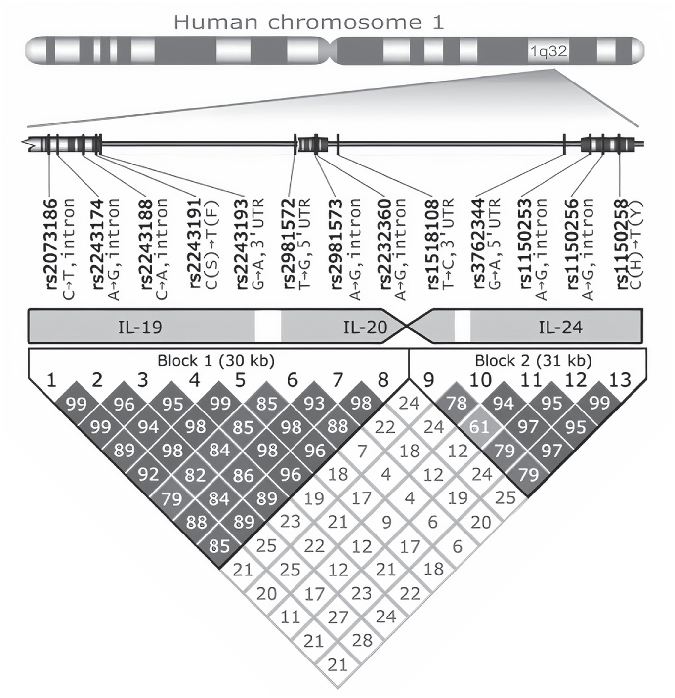
Representation of two haplotypes on chromosome 1. The region 1q32 on the chromosome (to the right) is amplified below it. The location and the two forms of each single-nucleotide polymorphism (SNP) are shown. For example, SNP rs2073186 occurs as either a C or a T. It is located in an intron, a noncoding part of a gene. SNP rs2243191 occurs as a C or T. It is located in a protein-coding region of a gene and causes a single amino acid (the building block of proteins) to change from S (serine) to F (phenylalanine). Below this amplification are shown the three genes in which the SNPs are located—IL-19, IL-20, and IL-24—as well as intergenic regions (in white). Shown below that are two linkage disequilibrium (LD) blocks (or haplotypes) in region 1q32. The numbers 1 to 13 correspond to the SNPs shown above. At the bottom is a grid showing the degree of LD between each pair among the 13 SNPs. The numbers in the boxes are coefficients of LD (D′), which range from 0 to 1. For example, D′ between SNP 1 (rs2073136) and SNP 3 (rs2243188) is .99, which indicates high LD. By contrast, D′ between SNP 6 (rs2981572) and SNP 9 (rs1518108) is only .07. Reprinted by permission from Springer: Genes & Immunity (Possible relations between the polymorphisms of the cytokines IL-19, IL-20 and IL-24 and plaque-type psoriasis. Kõks, S., Kingo, K., Vabrit, K., Rätsep, R., Karelson, M., Silm, H., & Vasar, E. Genes & Immunity, 6(5), 407–415. https://doi.org/10.1038/sj.gene.6364216), Copyright 2005.

Despite computational tools, estimating LD remains a significant challenge

Measures of LD are particularly sensitive to population-based differences in allele frequencies and the choice of a cutoff for minor allele frequency—that is, the level at which the less frequently occurring [minor] allele in a population is deemed rare and excluded from the analysis (Linck & Battey, 2019). Furthermore, researchers generally assume that to be in LD lead SNPs must be located no more than, for example, 50 kb apart. However, in what is known as long-range LD (LRLD), LD spans regions more than 1 Mb (1,000 kb) apart on a chromosome. The most familiar example of LRLD concerns a region of chromosome 6 known as the major histocompatibility complex, which plays a key role in the immune system, in which thousands of SNPs exhibit LRLD across a region greater than 1.5 Mb. Analysis has shown that LRLD of more than 5 Mb is common across the human genome (Nelson et al., 2020; Park, 2019). If LRLD is not considered, the result can be a significant overcounting of marker SNPs presumed to be independent (i.e., not in LD). It is worth noting that LRLD can be a sign of epistasis (G × G), a phenomenon that is hard to accommodate in an additive model (C. Zhang et al., 2017).

Further difficulties in estimating LD occur because they confound the assumption on which LD depends: that people have identical genomes in the somatic cells of their bodies. These difficulties include: De novo copy-number variations (CNVs) and duplications or deletions of segments of DNA ranging from more than 50 bp to several megabases. Such variations are estimated to encompass up to 9.5% of the human genome (Iourov et al., 2019; Zarrei et al., 2015). They are de novo because they are not inherited and can be unique to every individual. De novo copy-number variations can result in the duplication or deletion of whole genes. Researchers have identified approximately 100 genes for which both copies can be deleted in healthy persons without producing apparent phenotypic consequences. There is also extrachromosomal circular DNA, which are closed circles of DNA derived from chromosomal DNA that range in size from less than 100 bp to several kilobases and typically contain multiple active genes. Up to 10,000 extrachromosomal circular DNAs per cell have been identified in varying amounts and sizes and with different DNA sequences in all cell types (Ain et al., 2020); polyploidy, which occurs when cells have more than two complete sets of chromosomes, is found, to varying degrees, in normal human cells and tissues. For example, almost all adult ventricular cardiomyocytes, which form the muscle wall of the heart, are polyploid, typically containing four complete sets of chromosomes (Gan et al., 2020). More than 50% of liver cells (hepatocytes) exhibit polyploidy (S. Zhang et al., 2019), and most large bone marrow cells (megakaryocytes) contain up to 32 sets of chromosomes (Mazzi et al., 2018). The result of these and other phenomena is widespread somatic mosaicism—the existence of different genomes in different cells of the body. Somatic mosaicism is now known to be the normal human condition and is prevalent in the brain (Breuss, 2020; Kaeser & Chun, 2020; B. Zhao, Wu, et al., 2019).

Infinitesimal effects

What is perhaps most misleading about highlighting specific SNPs and using them to construct a schema of genetic neurodevelopmental etiology (of risk) is that according to researchers’ assumptions, the effect of any one of these SNPs on risk is minuscule (e.g., according to J. J. Lee et al. [2018], the marker SNP rs4860418 is associated with a .0071-unit decrease in genetic risk of EA. This effect size presumably matches that of the unknown causal-risk allele with which it is in LD). These effects are so small that it is inconceivable that the role of any of the unknown causal genetic variants could ever be demonstrated or analyzed experimentally. Of course, one could “knock out” the proposed gene in a mouse or find a family whose members lack the gene because of some rare condition and then connect the observed abnormal behavior with the phenotype under consideration. But this would simply be a way of distorting the findings by transforming what is insignificant and one effect among millions into the sole main effect.

To what extent is it biologically plausible, or even coherent, to assume that the cause of such a minuscule effect can be traced back to specific inherited DNA sequences? The problem with such an assumption is that in a complex biological system, the signal or signature of a minuscule effect will be irretrievably lost in a sea of effects. As the effect size of variation in specific DNA sequences diminishes, the effect size of all the other processes normally involved in shaping gene expression grows, including the entire developmental process. Such diminutive allelic effect sizes make sense only in the statistical realm, not the biological realm.

Replication

Given the assumption of a single set or core set of genetic risk factors for a given phenotype (Maier et al., 2018), it is important to consider whether identification of lead marker SNPs for a given attribute is consistently replicated across studies. Let us assume that in this context, “lead” means a marker SNP of genome-wide significance (at p ≤ 5 × 10^–8) that has a p value lower than those of all the other marker SNPs with which it is assumed to be in LD (according to whatever statistical procedures are used in this determination).

Consider eight large metanalyses of EA and/or intelligence/cognitive ability: (Davies et al., 2018; Hill, Marioni, et al., 2019; Kichaev et al., 2019; Lam et al., 2017, 2019; J. J. Lee et al., 2018; Okbay et al., 2016; Savage et al., 2018). Because EA is usually considered a proxy variable for intelligence, combining intelligence and EA should present no problems. Limiting ourselves to the unique marker SNPs found to have genome-wide significance in each study at p ≤ 5 × 10⁻⁸ yields 6,272 SNPs total across the eight studies. Of these, 5432, or 93.44%, occurred in only one study. (Table 1; see also the Supplemental Tables available online). ⁴

OPEN IN VIEWER

Table 1.

Lead SNPs for Intelligence and Educational Attainment Identified in Studies

Number of studies	Number of SNPs(N = 6,272)	SNPs (%)
1	5,432	93.44%
2	325	5.59%
3	43	0.74%
4	11	0.19%
5	2	0.03%
6	1	0.02%
7	0	0.00%
8	0	0.00%

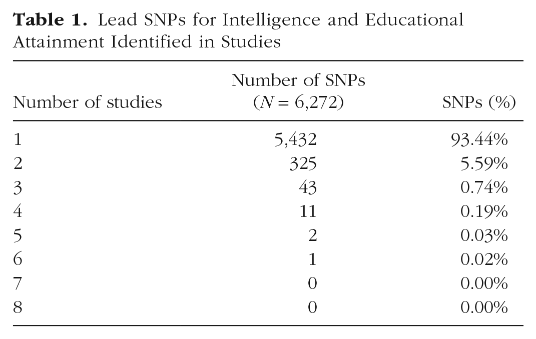
This poor record of replication of purportedly independent and lead marker SNPs of genome-wide significance goes largely unnoticed, even though these same SNPs are often used to construct schemas of genetic causation of risk and PRSs.

Basics

A PRS is intended to be a single-value estimate of a person’s genetic risk for an attribute (Choi et al., 2020). Take the example of constructing a PRS for EA. Suppose that a given GWAS (or combination of GWASs) contains information on 1 million marker SNPs for 100,000 persons as well as information on years of schooling completed. For each of the 100,000 members of the sample, the data would show the respondent’s EA and which SNP allele they possess for each of one million marker SNPs on a chip array. All these individual data could then be combined into “summary statistics,” which present the GWAS results in the form of population averages. For each SNP, the summary statistics identify the “effect” allele (A1; i.e., the marker SNP that shows a correlation with EA, which can be either positive or negative), the “no-effect” allele (A2), the frequency of A1 in the population, the average effect size of A1 on EA (an odds ratio for a dichotomous trait or a β for a quantitative trait), the standard error (SE), and the p value for the association. See Table 2 for an example.

OPEN IN VIEWER

Table 2.

Simplified Summary Statistics for a Single SNP Allele From a Hypothetical Study of Educational Attainment

Marker name (SNP)	A1(Effect allele)	A2	A1Frequency	Effect size	SE	p
rs4686944	G	T	0.02041	0.029	0.01087	.0441

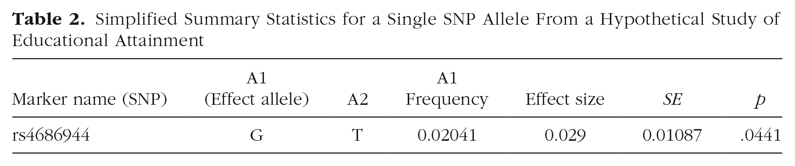
Suppose we wanted to construct a newborn’s PRS for EA (specifically, her odds of completing high school), and suppose her genotype for marker SNP rs4686944 in Table 2 was GG, which is two “effect” or “risk” alleles. On the basis of our summary statistics, we would multiply the effect size of this allele (0.02041) by the number of risk alleles she has (2). We would repeat this process for each of her 1 million marker SNPs (after accounting for LD) that showed an association with completion of high school and sum the results. In theory, the resulting value would tell us the newborn’s “genetic risk” for higher or lower EA. In 2018, Plomin and von Stumm wrote as if this capability was imminent:

IQ GPSs [genetic polygenic score; equivalent to PRS] will be used to predict individuals’ genetic propensity to learn, reason and solve problems, not only in research but also in society, as direct to consumer genomic services provide GPS information that goes beyond single gene and ancestry information. We predict that IQ GPSs will become routinely available from direct-to-consumer companies along with hundreds of other medical and psychological GPSs that can be extracted from genome-wide genotyping on SNP chips. (p. 155)

At present, however, PRSs for behavior have no individual predictive value whatsoever (Morris et al., 2020), and whether any PRS for any phenotype has individual predictive value is an open question. Instead, their ostensible predictive value concerns populations: A PRS is said to be predictive if the average PRS in a case population is higher than the average PRS in a control population, or if the average PRS of those, for example, in the lowest decile of EA is lower than those in the highest decile.

Plomin and von Stumm (2018) made these points clear when discussing a PRS they constructed to predict students’ performance on a United Kingdom–wide examination, the General Certificate of Secondary Education (GCSE), administered at the end of compulsory education at age 16 years. According to the authors, a scatterplot between GCSE scores and the PRS (Fig. 2a) shows “the difficulty of predicting individual outcomes when the correlation is modest (0.30 in this example)” (Plomin & von Stumm, 2018, p. 156). Squaring this correlation, they estimated that the PRS predicted 9% of the variance in risk in their study population but noted that

Although higher [PRSs] can be seen to predict higher GCSE scores on average, there is great variability between individuals. . . . Individuals within the lowest and highest [PRS] deciles vary widely in school achievement. . . . The overlap in the two distributions is 61%. (p. 156)

However, on a more optimistic note, they comment regarding their study sample “EA2” (Fig. 2c):

Despite this variability, powerful predictions can be made at the extremes. . . . Specifically, the average school achievement of individuals in the lowest EA2 GPS decile is at the 28th percentile. For the highest EA2 GPS decile, the average school achievement is at the 68th percentile. (p. 156)

OPEN IN VIEWER

Fig. 2.

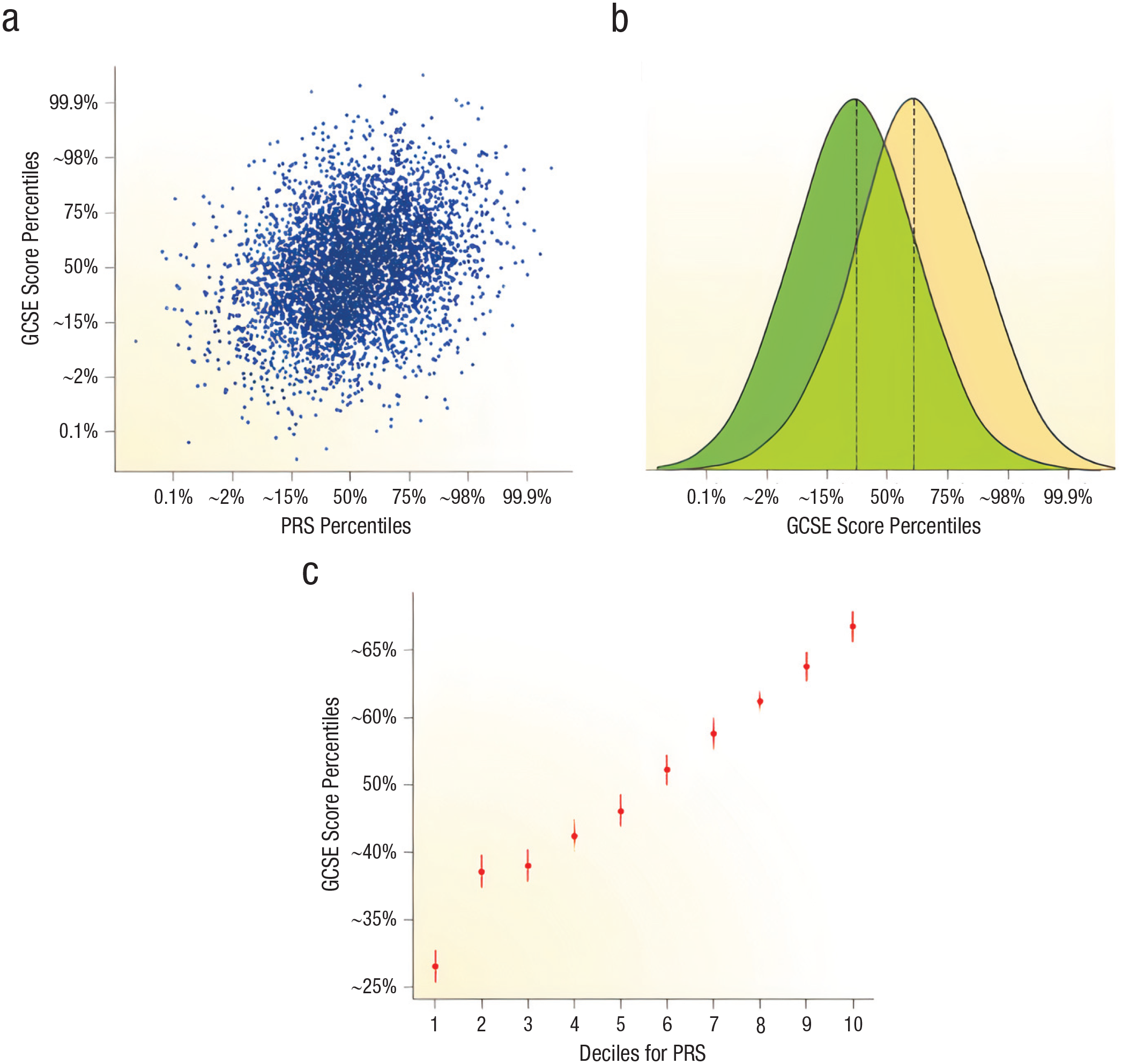
Polygenic risk scores (PRSs) and individual versus population prediction. The scatterplot in (a) shows the relationship between educational attainment (EA) PRS percentiles and General Certificate of Secondary Education (GCSE) score percentiles. “EA2” refers to a specific PRS in Plomin and von Stumm (2018). The graph in (b) shows that the population distribution of PRS is normally distributed; the average PRS of those who score higher on the GCSE is slightly higher. On this basis, the authors predict that their PRS predicts 9% of the variance in genetic risk. The overlap in the two distributions is 61%. In the graph in (c), the sample was divided into 10 equal-sized groups (deciles) on the basis of EA2 PRS and shows the relationship between average EA2 PRSs and average GCSE score. Reprinted by permission from Springer: Nature Reviews Genetics (The new genetics of intelligence. Plomin, R., & von Stumm, S. Nature Reviews Genetics, 19(3), 148–159. https://doi.org/10.1038/nrg.2017.104), Copyright 2018.

It is common practice to divide a PRS into lowest and highest deciles or quintiles and then note what seems like an impressive difference in the mean prevalence between the lowest and highest decile or quintile. But what may seem like an impressive difference is simply a general property of small correlations: Given large enough sample sizes, looking at the extremes will produce what appear to be large differences, even though the magnitude of the relationship is small. Finally, Plomin and von Stumm (2018), reflecting on the poor individual predictive power of their PRS, have recourse to a familiar refrain: “As bigger and better GPSs emerge, the predictive power will increase” (p. 156).

Estimating predictive performance is inferior to observing it in the real world

It is for these reasons that, according to the “gold standard,” before any claims that a PRS actually predicts anything can be made, a PRS developed on a training sample should be tested on a third sample entirely separate from both the discovery and training samples (Choi et al., 2020). Frequently, researchers do not do this. Sometimes, they will remove one or two study “cohorts” from their discovery sample (which consists of numerous cohorts), use these excluded cohorts as their training sample, and publish results derived from the training sample. To be sure, there are different statistical techniques designed to deal with the problem of model overfitting in the absence of a third independent sample and to estimate how accurately a predictive model will perform in practice. Cross-validation, for example, uses a single training sample that is then split into smaller “training” and “validation” subsets (Duncan et al., 2019). In discussing a recent study of the performance of cross-validation that was based on real-world data, Bauder et al. (2019) noted:

In real-world production applications, it is critical to establish a model’s usefulness by validating it on completely new input data and not just using the cross-validation results on a single historical data set. We present results for both evaluation methods, to include performance comparisons [and] find that using the separate training and [validation] sets generally outperforms cross-validation, indicating a better real-world model performance evaluation. (p. 19)

There is growing evidence that PRSs are overfit models. For example, Mostafavi et al. (2020) demonstrated that “the portability of a polygenic risk score can vary markedly depending on sample characteristics of both the original GWAS and the prediction set, and that this variation in prediction accuracy can be substantial” (p. 6). Variation in the samples for such things as the percentage of male versus female participants or the percentage of persons in various age or socioeconomic categories were all shown to substantially affect PRS accuracy.

Basics

In all the studies considered thus far, researchers employed data limited to persons of European ancestry. To be sure, PRSs have been constructed on the basis of discovery and training samples composed of persons of “Asian” or “African” descent. But care is taken to avoid “mixed” populations or, for example, using data derived from a GWAS of members of one ancestral group to construct a PRS for members of a different ancestral group. As J. J. Lee et al. (2018) note of their study:

Because the discovery sample used to construct the score consisted of people of European ancestry, we would not expect the predictive power of our score to be as high in other ancestry groups. Indeed, when . . . used to predict EA in a sample of African-Americans . . . the score only has an incremental R² of 1.6%, implying an attenuation of 85%. (p. 1115)

Researchers typically ascribe such R² attenuation to differences in genetic population characteristics between ancestral groups—differences in allele frequencies, haplotypes, degree of LD, and degree of genetic diversity (Duncan et al., 2019). These differences are the result of different population histories and are influenced by such phenomena as differences in migratory patterns, founder events, and population bottlenecks (loss of genetic variation that occurs when a new population is established by a very small number of people from a larger population), population expansions, relative population isolation, endogamy, inbreeding, adaptive pressures, and genetic drift (a random change in allele frequencies), to name a few. Genetic population characteristics are highly correlated with geography, although the sharing of certain allelic frequencies between populations need not entail a shared ancestry or geographic origin. Although researchers are aware of the existence of population genetic differences between as well as within ancestral populations (as typically defined), they believe they can effectively handle the latter (but not the former).

A population is structured when it contains subpopulations often, but not exclusively, distinguished by geographic location that exhibit systematic differences in population genetic characteristics (or allele frequencies). Persons of European ancestry are a structured population at every level, and the more fine-grained one’s analysis, the more that nested levels of population structure appear. For example, the ancestral population of the United Kingdom is composed of 17 distinct population “clusters” that are highly localized and differ in their population genetic characteristics (Leslie et al., 2015). Structured populations, which are most populations, are an omnipresent threat to the validity of genetic association studies because of population stratification.

Population stratification

Population stratification occurs when researchers mistake population genetic differences in allele frequencies for differences between case subjects and control subjects in risk alleles. Consider a simplified example—simplified in that it involves only one allele when a PRS can involve millions. Because of population genetic differences, the Roma have a higher percentage of the CYP2C19*2 allele (Petrovic et al., 2020). Suppose our phenotype was EA and the Roma were overrepresented in our study population. The Roma have, on average, much lower EA than other Europeans (Eurostat, n.d.). Hence, we might conclude that CYP2C19*2 is a risk allele for low EA. However, any association between CYP2C19*2 and EA would be the result of population stratification. Were we, for example, to exclude the Roma altogether from our sample, any correlation between CYP2C19*2 and EA would disappear (assuming, that is, that there were no other ancestral populations that exhibited similar population differences in CYP2C19*2 frequencies). The EA of the Roma are so low not because they have a high frequency of the CYP2C19*2 allele but because of their history as a persecuted and excluded minority (Van den Bogaert, 2018).

The two most widely used statistical methods for dealing with population structure are principal components analysis (PCA) and linear mixed modeling (LMM; Y. Zhang & Pan, 2015). PCA is used to identify patterns or “axes of variation” that explain the greatest amount of variance in allele (i.e., SNP) frequency in the sample. In a GWAS, what typically accounts for the greatest amount of variation in allelic frequency (the first principal component) is not the attribute of interest but the ancestries of the participants, which often correspond to geographical regions. Researchers adjust genotypes and phenotypes by amounts attributable to ancestry along each axis. It is common for researchers to do a PCA on the entire set of genotype data, then use the first 5, 10, 20, or more principal components as covariates in the association model. An alternative widely used approach is LMM, which incorporates both fixed and random effects, population structure being treated as a random effect.

There is strong evidence that neither of these approaches solves the problem of population stratification. For example, in several different studies, researchers reported that the average PRS for height increased from south-to-north across Europe (i.e., exhibited a “latitudinal cline”), paralleling average population differences in height from Italy to the Netherlands (Berg & Coop, 2014; Racimo et al., 2018; Robinson et al., 2015; Turchin et al., 2012; Zoledziewska et al., 2015). The results of these studies were highly touted not only as multiply replicated PRSs for height but also as an example of polygenic adaptation. Most of these studies were based on data assembled by an international collaborative effort known as the Genetic Investigation of ANthropometric Traits (GIANT) Consortium, consisting of the combined summary statistics from 79 individual GWASs totaling 253,288 persons of European ancestry from across Europe. In subsequent studies (Berg et al., 2019; Sohail et al., 2019), researchers attempted to replicate these findings using a larger sample from the U.K. Biobank.

The U.K. Biobank contains GWAS and “health and well-being” data of 500,000 volunteer participants from the United Kingdom. Researchers limited themselves to participants who self-identified as being of “white British ancestry” (N = 336,474). This study population was larger and more homogeneous, in terms of ancestry, than the population that constituted the GIANT Consortium from which the PRSs for height had been originally derived. Researchers failed to replicate the original findings. As Berg et al. (2019) noted of their results, “what once appeared an ironclad example of population genetic evidence for polygenic adaptation now lacks any strong support” (p. 14). Both Berg et al. (2019) and Sohail et al. (2019) concluded that the differences in the PRSs for height were picking up ancestral population differences in allele frequencies between, for example, the Italians and the Swedes, that had nothing to do with height. And they knew this because these scores did not identify differences in height (or at the very least, were significantly attenuated) in a more homogeneous population that contained neither Italians nor Swedes. Of their findings, Berg et al. (2019) commented that “methods for correcting for population stratification in GWAS may not always be sufficient for polygenic trait analyses” (abstract).

Doubts concerning the effectiveness of current methodologies in dealing with population stratification have continued. For example, the U.K. Biobank, a large segment of which has been assumed to represent a single relatively homogeneous population of persons of “white British ancestry,” itself exhibits population structure (Cook et al., 2020). This is not surprising given that, as noted above, “white British ancestry” does not constitute a structure-free population. Both Cook et al. (2020) and Haworth et al. (2019), showed that PRSs based on GWAS data from the U.K. Biobank for traits including education, income, body mass index (BMI), hypertension, smoking, and alcohol consumption were correlated with birth location. These associations with geography persisted even after they used PCA involving up to 100 principal components (Zaidi & Mathieson, 2020) and LMM. Differences in all these attributes—education, income, BMI, hypertension, smoking, and alcohol consumption—and many more are known to vary by geographic region throughout Great Britain. At the same time, allele frequencies are known to differ throughout Great Britain by geographic region because of differences in ancestral populations, which provides a source of covariance between genotype and attribute that will lead to population stratification. As Haworth et al. note (2019), “this phenomenon is important, both as a source of ecological-level covariance between genotypes and geographically heterogeneous complex traits and because of its apparent persistence across different analytical contexts and modes of statistical adjustment” (p. 6),

Researchers uncovered the same problem in analyzing PRSs for coronary artery disease, rheumatoid arthritis, schizophrenia, waist–hip ratio, body-mass index, and height in a Finnish population (Kerminen et al., 2019). Ancestral Finns are a population that, given the nature of their migratory history and relative isolation from the rest of Europe, one would expect to be more genetically homogeneous than “whites of British ancestry” (Kaariainen et al., 2017). Nonetheless, even after employing PCA and LLM, the authors observed strong correlations between the geographic distribution of the PRSs and Finnish population structure that runs from southwest to northeast.

Sibship studies

Researchers generally assume that studies of siblings from the same parents are immune to population stratification because genetic differences between siblings are due to the random partitioning of parental alleles (Selzam et al., 2019). Hence, it is common for researchers to attempt to replicate GWASs and PRSs using family studies. Many studies have shown that when a PRS score derived from a general-population GWAS discovery sample is applied to a sibling population, the R² significantly declines (J. J. Lee et al., 2018; Mostafavi et al., 2020; Trejo & Domingue, 2018). For example, J. J. Lee et al. (2018) noted a decline of 40% in their PRS when applied to a sibling study population. There have been numerous and at times convoluted attempts to explain this phenomenon, but the most straightforward is, in the words of Lello et al. (2020), that “at least some of the observed power in polygenic prediction among non-sibling people comes from effects such as subtle population stratification (perhaps correlated to environmental conditions or family socio-economic status)” (p. 9).

Zaidi and Mathieson (2020) demonstrated that if researchers use data from a general population GWAS discovery sample and develop a PRS using a sibling training sample, population stratification persists. Researchers have started to use sibling discovery samples to overcome this problem, and such studies have shown just how inflated population-based R² estimates are. For example, in a recent study of 159,701 siblings using sibling GWAS data (Howe et al., 2021), researchers observed that the within-sibships SNP heritability estimate for EA attenuated by 71% from the population estimate (population h² = 0.14; within-sibships h² = 0.04), while the estimate for cognition attenuated by 46% (population h² = 0.24; within-sibships h² = 0.13). Reported genetic correlations (for explanation, see Pleiotropy section below) between EA and height (Valge et al., 2019) and EA and BMI (Zeng et al., 2019), when reestimated with sibship data, were close to 0. The authors of this study (Howe et al., 2021) noted that “population estimates are likely to be driven by demography [i.e., population stratification] and indirect genetic effects” (p. 7).

Are sibling and family studies completely immune from population stratification, as is commonly assumed? They are not. It is known, for example, that in so-called admixed populations, stratification can persist in sibship studies (Mersha et al., 2015; Thornton et al., 2012; Wang et al., 2016). An admixed population is one in which members have recent ancestry from two or more separate sources. For example, as an “ancestral population,” African Americans arose within the past 400 years, and genome-wide ancestry estimates show averages of 73.2% African, 24.0% European, and 0.8% Native American ancestry (Bryc et al., 2015). Although persons of European ancestry are not an admixed population in this sense, the rise of multiracial and multiethnic children in the U.S. and Europe introduces admixture by degrees.

Proxy phenotypes

What kind of phenotypes are “income” and “EA”? According to Hill, Davies, et al. (2019), there are no risk alleles for income per se. Instead, there are risk alleles for attributes that are correlated with, and have a causal effect on, income:

Genetic variants do not act directly on income; instead, genetic variants are associated with partly heritable traits (such as intelligence, conscientiousness, health, etc.), which have their own complex gene-to-phenotype paths (including neural variables) and are ultimately associated with income. (p. 19)

Indeed, the idea of a phenotype “income,” apart from all behaviors and features of persons that might influence it, and apart from the particular social, political, and economic institutions in which income exists and its distribution occurs, is nonsensical. Furthermore, as Hill, Davies, et al. (2019) note, any correlation between a given attribute (e.g., intelligence or health) and income is socially and historically contingent: Income could just as well depend on service to the party, and continually shifting political policies can alter, if not eliminate, the degree of correlation between income and health. The same is true of EA. The grade one completes in a particular educational system (i.e., EA), in addition to being correlated with various socioeconomic factors, is correlated with different behavioral and health-related attributes, some of which exert a causal influence on EA and may also be heritable. But “the grade one completes” is not itself a phenotype that influences the grade one completes in addition to these behavioral and physical attributes. It is for such reasons, presumably, that EA is treated as a proxy phenotype (Rietveld et al., 2014): “Educational attainment is a good proxy phenotype for cognitive performance, because cognitive performance is strongly genetically influenced and causally affects educational attainment” (p. 13791).

PRSs for proxy phenotypes such as income and EA can, presumably, predict heritable attributes with which income and EA are correlated and that exert a casual influence on them. However, income and EA are also commonly said to be “genetically correlated,” not only with each other and with intelligence but also with a host of other attributes. How is this possible? Inasmuch as there is now an explosion of studies exploring genetic correlations between phenotypes, this is a question of some importance.

Pleiotropy

Genetic correlation, or “genetic overlap,” is a measure of the proportion of variance that two traits share as a result of shared risk alleles (Hackinger & Zeggini, 2017). It is taken as an indication of pleiotropy, the phenomenon in which the same allele serves as a risk factor for two different phenotypes. Researchers typically divide pleiotropy into horizontal pleiotropy and vertical (or mediated) pleiotropy.

Horizontal pleiotropy

Horizontal pleiotropy (Fig. 3a) occurs when two or more traits share a certain percentage of risk alleles. It can serve as an explanation for their phenotypic correlation or co-occurrence: They co-occur because their risk alleles are shared and hence inherited together. If genetic correlations are sufficiently high, a PRS for one trait can predict a certain percentage of the variance of the correlated trait. So called cross-trait PRSs have become a popular technique to measure the genetic similarity of polygenic traits (Leppert et al., 2020; Pouget et al., 2019). In the current context, claims of genetic correlation do not concern the correlation of known risk alleles (which, it will be recalled, are not identified in GWASs). Rather, it is a correlation between marker alleles and a given trait. The marker SNPs the two traits have in common are assumed to be in LD with the same risk alleles (van Rheenen et al., 2019), but there is no way that researchers can know this to be the case.

OPEN IN VIEWER

Fig. 3.

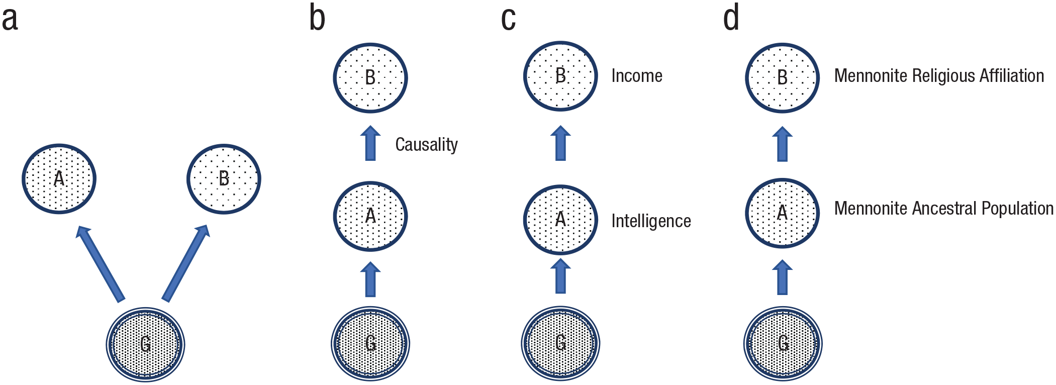
Horizontal and vertical pleiotropy. In horizontal pleiotropy (a), two attributes, A and B, are correlated because they share a certain percentage of genetic risk alleles. In vertical pleiotropy (b), two attributes, A and B, are correlated not because they share genetic risk alleles, but because A has a causal influence on B. B could be heritable with its own risk alleles that are distinct from A’s, or it could be nonheritable and without any risk alleles, as in the case of income. In (c), the relationship between intelligence and income is depicted as an example of vertical pleiotropy. In (d), the relationship between being a member of a specific Central European subpopulation and having a Mennonite religious affiliation is depicted as an instance of vertical pleiotropy.

An abundance of correlations

With more genetic correlation studies have come ever more reports of genetic correlations (whether horizontal or vertical). Intelligence, for example, has been reported to be significantly positively genetically correlated with, among other things, EA, income, autism, short-sightedness, cheese intake, eating Muesli cereal, grip strength in the right hand, age at first birth, longevity, parental longevity, voting behavior, anorexia nervosa, wearing glasses or contact lenses, subjective well-being, intracranial volume, height, drinking ground coffee, belonging to a religious group as a leisure activity, and iron and magnesium levels, and to be negatively correlated ⁶ with type 2 diabetes, schizophrenia, hyperopia, bipolar disorder, Alzheimer’s disease, obesity/BMI, number of children, neuroticism, major depressive disorder, coronary artery disease, heart attack, ischemic and large vessel disease stroke, bipolar disorder, attention-deficit/hyperactivity disorder, osteoarthritis, hypertension, levels of C-reactive protein (a protein made in response to inflammation), and lung cancer (Aaroe et al., 2021; Abbott et al., 2021; Davies et al., 2018; Engen et al., 2020; Hagenaars et al., 2016; Hill, Davies, et al., 2019; Hill, Marioni, et al., 2019; Ligthart et al., 2018; Savage et al., 2018; Valge et al., 2019; Y. Zhao, Ning, et al., 2019). Given the number of correlations, when researchers claim that a PRS predicts intelligence, how do they know they are predicting intelligence (however precisely this is measured) and not one or more of the above?

Many findings of genetic correlations are contradictory and/or have not been consistently replicated. For example, Engen et al. (2020) report no negative genetic correlation between intelligence and schizophrenia; Hill, Davies, et al. (2019) report no genetic correlation between intelligence and subjective well-being; and Hill, Marioni, et al. (2019) report no negative genetic correlation between intelligence and bipolar disorder. In a study using sibship data, Howe et al. (2021), report no genetic correlation between intelligence and height, BMI, and levels of C-reactive protein. It is often assumed that high genetic correlations entail high phenotypic correlations (an assumption known as “Cheverud’s conjecture” [Cheverud, 1988]). But such need not be the case. For example, in a study of assorted psychiatric conditions, Roelfs et al. (2021) noted that a large portion of significant genetic correlation occurred between attributes that were phenotypically uncorrelated. This might help explain seemingly contradictory findings. For example, researchers have reported a positive genetic correlation between autism and EA (Grove et al., 2019), although phenotypically, the correlation is negative (Toft et al., 2021). Autism has also been genetically correlated, in different studies, with both higher intelligence (Bulik-Sullivan et al., 2015; Clarke et al., 2016) and intellectual disability (Jensen et al., 2020). A phenotype may show a positive genetic correlation with one of two genetically correlated traits and a negative correlation with the other. For example, schizophrenia is frequently reported to be genetically correlated with lower general cognitive function and higher EA (Lam et al., 2019; Ohi et al., 2018; Savage et al., 2018), even though higher general cognitive function and higher EA are reported to be highly genetically and phenotypically correlated.