Associative interference and nonreinforcement in human contingency learning

Abstract

This article reports three experiments comparing the impact on contingency assessment of associative cue interference (proactive, interspersed, and retroactive) and nonreinforcement (latent inhibition, partial reinforcement, and extinction). All three experiments used variants of the rapid trial streaming procedure developed by Allan and collaborators. Participants were exposed to stimulus streams and then asked how likely it was for a target cue to be accompanied (Experiment 1) or to be followed (Experiments 2 and 3) by a target outcome. Experiments 1 and 2 looked at interference and found that when the objective target cue–outcome contingency is positive, interspersed interference is more effective than either proactive or retroactive interference. Experiment 2 additionally showed that this conclusion was a function of the target cue–outcome contingency: when the number of cue–outcome pairings was low, retroactive interference was more efficient than interspersed interference. Experiment 3 examined nonreinforcement and found that the efficacies of latent inhibition, partial reinforcement, and extinction are also a function of the target cue–outcome contingency, but the pattern differed greatly from what was observed in Experiment 2. When the number of cue–outcome pairings was high, there was no difference between latent inhibition, partial reinforcement, and extinction. When the number of cue–outcome pairings was low, extinction did not lower the contingency judgement, whereas latent inhibition and partial reinforcement did.

Keywords

Associative interference cue interference interspersed interference nonreinforcement contingency learning

In Pavlovian conditioning, an initially neutral conditioned stimulus (CS) is paired with a biologically relevant unconditioned stimulus (US), causing the CS to subsequently trigger a conditioned response. In contingency learning, after being exposed to a series of stimuli, a participant is asked whether a specific stimulus (a cue) can be used to predict the occurrence of another stimulus (an outcome). Like Pavlovian conditioning, contingency learning reflects the ability of living organisms to extract statistical regularities from their environment and to potentially use this knowledge to predict what comes next or what accompanies what (Dickinson, 1980; Rescorla, 1988; Shanks, 1995).

The objective predictive value of the CS/cue relative to the absence of the CS/cue (contingency), as calculated through the ∆p metric, tracks many effects in the associative literature better than other algebraic measures of relatedness (e.g., Allan & Jenkins, 1983; Granger & Schlimmer, 1986; Hallam et al., 1992; Rescorla, 1968), especially effects that result from variations in the probability of the US/outcome given the CS/cue, and variations in the probability of the US/outcome (hereafter “outcome”) given the absence of the CS/cue (hereafter “cue”) as:

Δ p = \frac{a}{a + b} - \frac{c}{c + d}

where a is the number of trials in which the cue and the outcome have been presented together, b is the number of trials in which the cue has been presented without the outcome, c is the number of trials in which the outcome has been presented without the cue, and $d$ is the number of trials in which neither the cue nor the outcome has been presented. The cue is an objective predictor of the outcome when ∆p is positive (positive contingency), whereas it is an objective predictor of the absence of the outcome when ∆p is negative (negative contingency). When ∆p is null (null contingency), the cue is uninformative concerning the occurrence of the outcome. Both the potential of a CS to elicit conditioned responding (Rescorla, 1967, 1968) and contingency judgements are reasonably well tracked by ∆p in most dyadic situations (for reviews, see Shanks, 1995, 2007). Note that we use ∆p here to facilitate exposition, not as an account of how associative interference and nonreinforcement decrease acquired behaviour.

One way to lower the value of ∆p, and hence to reduce conditioned responding and contingency judgements, is to increase the number of b-trials (i.e., cue present, outcome absent). This can be done by either presenting the cue alone (i.e., nonreinforcement) or presenting the cue with a nontarget outcome (i.e., associative interference). Considering nonreinforcement, there are three temporal relationships that can exist with respect to target training. In latent inhibition (LI) treatment, the cue-alone presentations occur prior to the pairings of the cue with the target outcome; in partial reinforcement (PR) treatment, the cue-alone presentations occur interspersed with the pairings of the cue and target outcome; and in extinction (Ext) the cue-alone presentations occur after the pairings of the cue and the outcome. Considering associative [outcome] interference, once again three different temporal relationships can be identified. In proactive interference (PI) the cue is paired with a potentially interfering, nontarget outcome before the pairings of the cue with the target outcome; in interspersed interference (II) the cue is presented with a nontarget outcome interspersed among the pairings of the cue and target outcome; in retroactive interference (RI) the cue is paired with an interfering outcome after it has been paired with the target outcome. Much RI research has focused on the case of counterconditioning (CC) in which the valence of the interfering US is opposite that of the target US (reviewed in Jozefowiez et al., 2020).

LI, PR, and Ext have each been extensively studied in isolation, with the literature heavily weighted towards Ext due to the potential practical applications of the procedure. Critically, there has been no systematic comparison of the relative efficacies of LI, PR, and Ext (but see Miller et al., 2015; Pineño & Miller, 2005, for studies that examine both LI and Ext). Research concerning associative interference with respect to conditioning and contingency learning has focused on interference between events trained sequentially across different phases of treatment (for reviews, see Miller & Escobar, 2002; Polack et al., 2017), that is, PI and RI. II seems to have been completely neglected at both the theoretical and empirical levels. For example, nothing is known concerning its robustness relative to PI and RI. Finally, there has been no systematic comparison of the several types of nonreinforcement with the several types of associative interference, with the notable exception of papers contrasting Ext and CC (reviewed in Jozefowiez et al., 2020) which, collectively, seem to conclude that CC is more efficient than Ext (but see Jozefowiez et al., 2020, for boundary conditions to this conclusion; also see Hall & Pearce, 1979, for a related comparison between PI and LI).

The goal of the present article is to provide the first systematic comparison of the relative strengths of the LI, PR, and Ext effects on one hand, and the PI, II, and RI effects on the other, at least within the context of a specific contingency assessment task: the streamed-trial procedure developed by Allan and her collaborators (Crump et al., 2007; Hannah et al., 2009; Siegel et al., 2009). In this task, the participants are exposed to rapid flows of cues and outcomes at the end of which they are asked to assess the contingency between the target cue and the target outcome. One advantage of this task over other contingency judgement tasks is that the short duration of the stimuli facilitates fully within-subject designs, even with many conditions. Experiments 1 and 2 contrast PI, II, and RI; Experiment 3 extends the strategy of the first two experiments to compare LI, PR, and Ext.

As our aim is to bring empirical grist to the theoretical mill, this article remains agnostic regarding the learning process, notably the question of whether Pavlovian conditioning reflects the formation of “associations” between stimulus representations (e.g., Denniston et al., 2001; Mackintosh, 1975; Pearce & Hall, 1980; Rescorla & Wagner, 1972; Wagner, 1981) or not (e.g., De Houwer, 2009; Gallistel & Gibbon, 2000). Otherwise, it might seem to the reader that our data are relevant only if one adopts the same theoretical orientation as us. We use terms like “nonreinforcement,” “associative interference,” “latent inhibition,” and so on, purely descriptively, without making any assumptions regarding the underlying mechanisms. For instance, “nonreinforcement” merely refers to the operation in which the cue is presented without the outcome, and “associative interference,” refers to the operation in which the cue is paired with another outcome. Whether the same mechanism underlies “nonreinforcement” and “associative interference” and whether this mechanism can best be described in associative terms is not our concern in this article, although we hope that in the long term, our data will facilitate resolution of these questions.

Experiment 1

Experiment 1 contrasted PI, II, and RI using an associative streamed-trial procedure in which short-duration events (of trial types a, b, c, and d) are presented in uninterrupted streams. The procedure used in Experiment 1 was similar to those used in previous streaming experiments (e.g., Jozefowiez et al., 2020; Murphy et al., 2021) in its use of somewhat longer stimuli than earlier streaming experiments (Crump et al., 2007; Hannah et al., 2009; Jozefowiez, 2021; Jozefowiez et al., 2022; Laux et al., 2010; Maia et al., 2018; Siegel et al., 2009). In the present experiments, testing of the cue–outcome relationship occurred immediately after training. It is well-established that tests immediately after learning favour recency effects, so we expected PI to be weaker than II, and II to be weaker than RI. Many preliminary studies were conducted before Experiment 1, which sought a procedure and parameters that would be sensitive to PI so floor effects could be avoided. Once we found a procedure that yielded PI, Experiment 1 was conducted.

The design of Experiment 1 is summarised in Table 1. The experiment included four critical conditions: Control (Ctl), PI, II, and RI. In all four critical conditions, participants rated the contingency between a cue (C) that would be the target of associative interference and its target outcome (O3). C and O3 were paired in Phase 2 of all conditions. In the PI condition, extensive interfering C-O2 trials were administered during Phase 1. In the II condition, extensive interfering C-O4 trials were administered during Phase 2. In the RI condition, extensive interfering C-O6 trials were administered in Phase 3. In the Ctl condition, C was not paired with any outcome other than O3 in Phase 2. In all conditions, all three phases of treatment were perfectly matched in terms of number of trials and types of trials except for the presence of potentially interfering trials (C-O2, C-O4, or C-O6) and, when a phase of a condition lacked C-O2, C-O4, or C-O6 trials, an irrelevant cue was substituted for C. This was done to minimise the role of factors other than associative interference. Thus, the design of Experiment 1 permitted us to compare PI, II, and RI on a level playing field except for differences in the temporal order of relevant trials and recency between interfering training and test. In addition to those critical experimental conditions, Experiment 1 included a warm-up condition that always came first and five dummy conditions that served to expose participants to a wide range of possible cue–outcome contingencies in each of the three phases.

Table 1.

Number and type of trials for the streams used in Experiment 1.

Condition	Trial composition
Warm-up (LHL)	Phase 1: 2 A-O1/8 A- (core) + 19 B-O2 (filler)
	Phase 2: 8 C-O3/2 C - (core) + 20 D-O4 (filler)
	Phase 3: 2 E-O5/8 E - (core) + 20 F-O6 (filler)
Ctl (HHH)	Phase 1: 8 A-O1/2 A - (core) + 40 B-O2 (filler)
	Phase 2: 8 C-O3/2 C - (core) + 40 D-O4 (filler)
	Phase 3: 8 E-O5/2 E - (core) + 40 F-O6 (filler)
PI (HHH)	Phase 1: 8 A-O1/2 A - (core) + 40 C-O2 (interfering)
	Phase 2: 8 C-O3/2 C - (core) + 40 D-O4 (filler)
	Phase 3: 8 E-O5/2 E - (core) + 40 F-O6 (filler)
II (HHH)	Phase 1: 8 A-O1/2 A - (core) + 40 B-O2 (filler)
	Phase 2: 8 C-O3/2 C - (core) + 40 C-O4 (interfering)
	Phase 3: 8 E-O5/2 E − (core) + 40 F-O6 (filler)
RI (HHH)	Phase 1: 8 A-O1/2 A - (core) + 40 B-O2 (filler)
	Phase 2: 8 C-O3/2 C - (core) + 40 D-O4 (filler)
	Phase 3: 8 E-O5/2 E - (core) + 40 C-O6 (interfering)

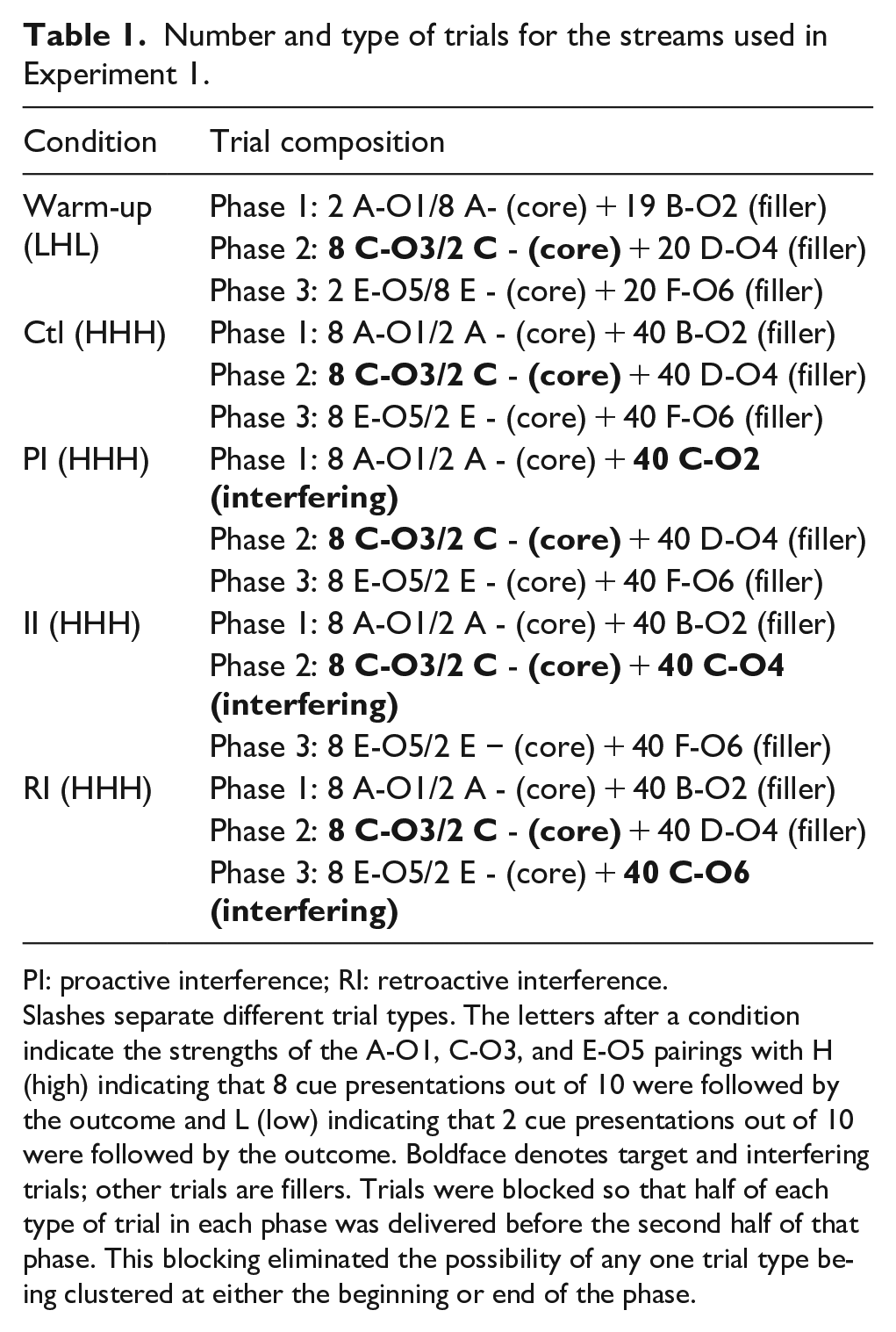
PI: proactive interference; RI: retroactive interference.

Slashes separate different trial types. The letters after a condition indicate the strengths of the A-O1, C-O3, and E-O5 pairings with H (high) indicating that 8 cue presentations out of 10 were followed by the outcome and L (low) indicating that 2 cue presentations out of 10 were followed by the outcome. Boldface denotes target and interfering trials; other trials are fillers. Trials were blocked so that half of each type of trial in each phase was delivered before the second half of that phase. This blocking eliminated the possibility of any one trial type being clustered at either the beginning or end of the phase.

Method

Participants

Experiment 1 was conducted online using the Gorilla Experiment Builder (www.gorilla.sc) to create and host the experiment (Anwyl-Irvine et al., 2020). Based on effect sizes in prior pilot experiments, we aimed at recruiting 130 participants. Participants were recruited from two different populations: the SUNY-Binghamton subject pool and Amazon MTurk. Participants were not recruited unless they were between 18 and 50 years old with no prior history of, or predisposition towards, visually induced epileptic seizures. A total of 52 participants were recruited from the SUNY-Binghamton subject pool and received course credit for their participation; 51 met a learning criterion based on performance in the pre-experimental warm-up phase and were included in the statistical analyses (M_age: 19 ± 0.89, min: 18, max: 22; 26 males, 25 females). The remaining 78 participants were recruited through Amazon MTurk and were paid US$6.00 for their participation. They were constrained to be English native speakers living in the United States, United Kingdom, Canada, Australia, or New Zealand: 74 participants met the learning criterion (age: 34.97 ± 7.06, min: 19; max: 50; 44 males, 30 females, 1 participant preferred to not provide gender information). Thus, the results reported are based on 125 participants. All experiments reported were approved by SUNY-Binghamton’s Institutional Review Board.

Apparatus

The procedure was composed of a warm-up condition which always came first, plus four experimental conditions and five dummy conditions in an order randomised for each participant. Each condition used a different set of cues (A, B, C, D, E, F) and a different set of outcomes (O1, O2, O3, O4, O5, O6). The cues and outcomes were all simple 300 × 300 pixels images of distinctly different objects. The cues belonged to the following semantic categories: fruits/vegetables, road signs, non-threatening animals, clothing, hieroglyphics, and transportation devices. The outcomes belonged to the following semantic categories: furniture, buildings, musical instruments, adinkra symbols, school-related objects, and toys. For all participants, each family of cues was randomly paired without replacement with a family of outcomes and within each of these paired families, 10 cue/outcome dyads were created. Then for each participant anew, one cue/outcome dyad from each of the six paired families was assigned to each condition, following which the role of each of these six cue/outcome dyads was randomly assigned without replacement to each functional role (i.e., A-O1, etc.).

Procedure

Warm-up

The warm-up condition preceded all experimental and dummy conditions. The warm-up condition was intended to train the participants to judge simple contingencies and minimise any “special” status of the first condition experienced. After giving their consent to participate in the study, entering their age and gender, reading a short instructional screen asking them to turn off their cellphones and avoid distractions for the next 30 min, participants were exposed to a stimulus stream. This stream was preceded by written instructions telling participants to keep their eyes on a fixation cross that would appear on the centre of a computer screen and to use the computer mouse to click on a button at the bottom of the screen to start the stimulus streams. The stream was composed of three 30-trial phases (due to a programming error, Phase 1 of the warm-up condition consisted of only 29 trials, instead of the 30 intended) during which a fixation cross (black on a white screen) remained visible at the centre of the screen. The trial composition of each phase is shown in Table 1. Each phase was composed of a set of 10 core trials aimed at establishing a basic contingency between a target stimulus (stimulus A in Phase 1, stimulus C in Phase 2, stimulus E in Phase 3) and a target outcome (O1 in Phase 1, O3 in Phase 2, O5 in Phase 3), plus 20 filler trials involving different cues and outcomes in each phase. A trial consisted of a simultaneous presentation of a cue and outcome (or a cue alone) for 450 ms, followed by a 300-ms intertrial interval (ITI). With simultaneous stimulus presentations, the terminology of “cue” and “outcome” might appear odd, but as used here it merely reflects the rating questions which asked: “If [image of cue] was presented, how likely is it that [image of outcome] would be presented with it?” On odd training trials, the cue appeared in the upper left corner of the screen, while the outcome appeared in the upper right corner of the screen. On even trials, the cue appeared in the lower left corner of the screen, while the outcome appeared in the lower right corner. For any given type of trial, half of the trials belonged to the even set (with stimuli presented in the lower part of the screen), whereas the other half belonged to the odd set (with stimuli presented in the upper part of the screen). The order of the trials within each set within each phase was determined randomly. The training trials in each phase were presented in two equivalent blocks to reduce the possibility of any one trial type being unduly clustered at the beginning or end of that phase of training.

At the end of the stream, participants were asked to judge the A-O1, C-O3, and E-O5 contingencies, with the order of testing determined randomly in each condition for each participant. In the sentence, “If [image of cue] was to be presented, how likely is it that [image of outcome] would be presented with it?”, the cue and outcome images were the actual images that played the roles of A, C, and E, and O1, O3, and O5. Below the question was a Likert-type scale ranging from 0 to 100 (incremented in steps of 10), and anchored at 0 (Unlikely) and 100 (Highly likely). Participants had to click on the Likert-type scale and then on a button reading “Continue” to either see the next contingency judgement for that condition or start the training for the next condition. Clicking on the Continue button ensured that the cursor was at the same point when each question was presented. The contingency rating of C-O3 was the target cue-outcome dyad, but we asked about A-O1 and E-O5 as well so that across successive conditions, participants would not learn to focus excessively on Phase 2 of training, at the cost of attention to Phases 1 and 3.

Experimental conditions

Experimental conditions began immediately after the last contingency rating in the warm-up condition. Each participant was exposed to nine conditions, identical to the one they had experienced during the warm-up, except for the trial composition. Five of those conditions were “dummy” conditions that were of no particular interest. They were included only so that participants would be repeatedly exposed to low (2 out of 10 cue presentations paired with their outcomes) and high (8 out of 10 cue presentations paired with their outcomes) cue–outcome contingencies and hence become accustomed to using a large range of the Likert-type scale. The trial composition for those streams is provided in the online supplementary material. The trial composition for the four experimental streams (Ctl, PI, II, RI) is depicted in Table 1. Just like for the warm-up stream, each phase of those streams was composed of a set of core trials: these core trials were intended to establish a strong contingency between the target cue and the target outcome specific to each phase (A and O1 in Phase 1, C and O3 in Phase 2, E and O5 in Phase 3). In the Ctl condition, 40 filler trials were added to each phase, as was done during the warm-up. In the interference conditions (PI, II, RI), one of these sets of filler trials was replaced by a set of interfering trials aimed at impacting the expression of the C-O3 contingency trained in Phase 2. During those interfering trials, stimulus C was paired with another outcome other than O3. They occurred in Phase 1 in the PI stream (before the training of the C-O3 contingency), in Phase 2 within the II stream (while the C-O3 contingency was being trained), and in Phase 3 in the RI streams (after the C-O3 contingency has been trained). In all conditions, participants had to rate the A-O1, C-O3, and E-O5 contingencies. Only the C-O3 contingency was of focal interest to us, but the ratings of the A-O1 and E-O5 contingencies were requested to encourage participants to pay equal attention to each phase of training, and these ratings as well as those in the dummy conditions served as validity checks. The order of presentation of the nine conditions following the warm-up condition was determined randomly for each participant.

Attention and distraction screens

In light of the very large differences in objective contingencies between C-O3 on one hand and A-O1 and E-O5 on the other during the warm-up condition, participants who gave the same ratings for the A-O1, C-O3, and E-O5 contingencies were excluded from the analysis. In addition to the 125 participants whose data were retained, the warm-up exclusion criterion led to the elimination of 5 participants. Once participants had been exposed to all 10 conditions, they were presented with a screen at the bottom of which were 5 stimuli (a blob, a circle, a crescent, a square, and a hexagon). These shapes were solid black and appeared over a white background. Participants were asked to click on the square. They were then asked whether they devoted their full attention to the task. Participants who failed to click on the square (n = 1) or said that they had been distracted during the task (n = 7) were also eliminated from the study. All the participants were then shown a debriefing screen that thanked them for participating and explained in general terms the purpose and design of the study.

Data analysis

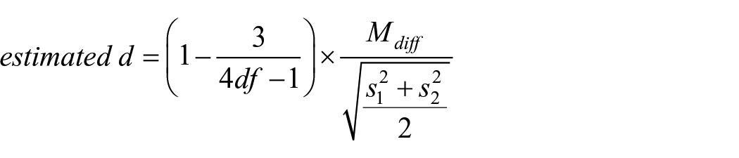
Inferential analyses were based on a repeated-measure analysis of variance (ANOVA). The Huyhn–Feldt correction was applied when the sphericity assumption was not met. The partial eta-squared statistic ( $η_{p}^{2}$ ) and its 90% confidence interval (CI) were used to estimate the effect size for each effect in the ANOVA. They were computed using resources in Nelson (2016; see Steiger, 2004, for why 90% CIs should be used if an alpha of .05 is set for the ANOVA). Cohen’s d was used as an effect size whenever two conditions were compared. The unbiased estimate of Cohen’s d in the population (sometimes called Hedge’s g) was used as a measure of effect size. Following Cummings’ (2012) recommendation it was computed with the formula:

e s t i m a t e d d = (1 - \frac{3}{4 d f - 1}) \times \frac{M_{d i f f}}{\sqrt{\frac{s_{1}^{2} + s_{2}^{2}}{2}}}

where the right side of the formula divides the mean of the difference scores across participants ( $M_{d i f f}$ ), by an estimate of standard deviation that considers the pooled variances of the two conditions, $\sqrt{\frac{s_{1}^{2} + s_{2}^{2}}{2}}$ , and df is the degrees of freedom on which a paired samples t-test is based (n– 1). The left side of the formula applies a correction for estimating d based on a sample .95% CIs for Cohen’s d for paired designs can only be approximated. Cousineau and Goulet-Pelletier (2021) reviewed eight different methods to achieve this goal with the conclusion that the best one is the adjusted lambda-prime method. This method was implemented using the ESCI module for JAMOVI (www.jamovi.com). We also report the correlations between pairs of conditions as this information might prove useful in future power analysis.

Error bars in our graphs are 95% CIs computed using Student’s t distribution. The raw data for this and the subsequent experiments are available at https://orb.binghamton.edu/jwhswcm_rawdata/1. Effects sizes, both in the original units and standardised ones (Cohen’s d) are reported in the table of results. Although a 95% CI provides more information than a t-test, a t-test would be significant at the standard .05 significance threshold if 0 is not within the 95% CI (Cummings, 2012).

Results

Only results concerning the C-O3 ratings in the Ctl, PI, II, and RI conditions will be presented here. Results concerning the C-O3 ratings in the dummy and warm-up conditions and the A-O1 and E-O5 ratings can be found in the online supplementary materials.

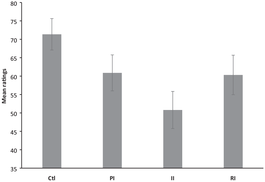
Figure 1 shows the ratings for the C-O3 contingency in the Ctl, PI, II, and RI conditions. A repeated-measures ANOVA found a statistically significant effect of the interference treatment (Ctl vs. PI vs. II vs. RI), F(3, 370.80) = 13.50, p < .001, $η_{p}^{2}$ = .10, 90% CI = [0.05, 0.14]. As shown in Table 2, the C-O3 contingency was rated lower in each of the interference conditions, PI, II, and RI, compared with the Ctl condition. There was no detectable difference between PI and RI, whereas II proved more efficient at lowering the rating of the C-O3 contingency than either PI or RI.

Figure 1.

Mean ratings for the C-O3 contingency in the Ctl, PI, II, and RI conditions in Experiment 1. Error bars are 95% CIs.

Table 2.

Results of Experiment 1.

Subjects	Comparison	M difference	Cohen’s d	Between-measurement r
All	Ctl vs. PI	10.50 [4.72, 16.20]	0.40 [0.18, 0.63]	.21
All	Ctl vs. II	20.60 [14.20, 26.90]	0.78 [0.53, 1.03]	–.08
All	Ctl vs. RI	11.00 [4.53, 17.60]	0.40 [0.16, 0.64]	.10
All	PI vs. II	10.10 [3.85, 16.30]	0.36 [0.14, 0.58]	.10
All	PI vs. RI	0.56 [–6.34, 7.46]	0.02 [–0.22, 0.26]	.21
All	II vs. RI	–9.52 [–16.10, –2.92]	–0.32 [–0.55, –0.10]	.20
MTurk	Ctl vs. PI	3.51 [–3.25, 10.30]	0.15 [–0.14, 0.44]	.21
MTurk	Ctl vs. II	17.40 [8.46, 26.40]	0.65 [0.32, 1.00]	–.06
MTurk	Ctl vs. RI	4.05 [–4.04, 12.20]	0.15 [–0.15, 0.46]	.13
MTurk	PI vs. II	13.90 [5.43, 22.40]	0.51 [0.20, 0.84]	.08
MTurk	PI vs. RI	0.54 [–7.51, 8.59]	0.02 [–0.28, 0.32]	.16
MTurk	II vs. RI	–13.40 [–21.70, –5.11]	–0.45 [–0.73, –0.17]	.28
SUNY	Ctl vs. PI	20.60 [10.80, 30.30]	0.73 [0.39, 1.10]	.25
SUNY	Ctl vs. II	25.10 [16.40, 33.80]	0.96 [0.62, 1.34]	.29
SUNY	Ctl vs. RI	21.20 [10.70, 31.70]	0.76 [0.39, 1.17]	.07
SUNY	PI vs II	4.51 [–4.65, 13.70]	0.16 [–0.16, 0.48]	.33
SUNY	PI vs. RI	0.59 [–12.00, 13.20]	0.02 [–0.40, 0.44]	–.15
SUNY	II vs. RI	–3.92 [14.90, 7.10]	–0.14 [–0.54, 0.25]	–.02

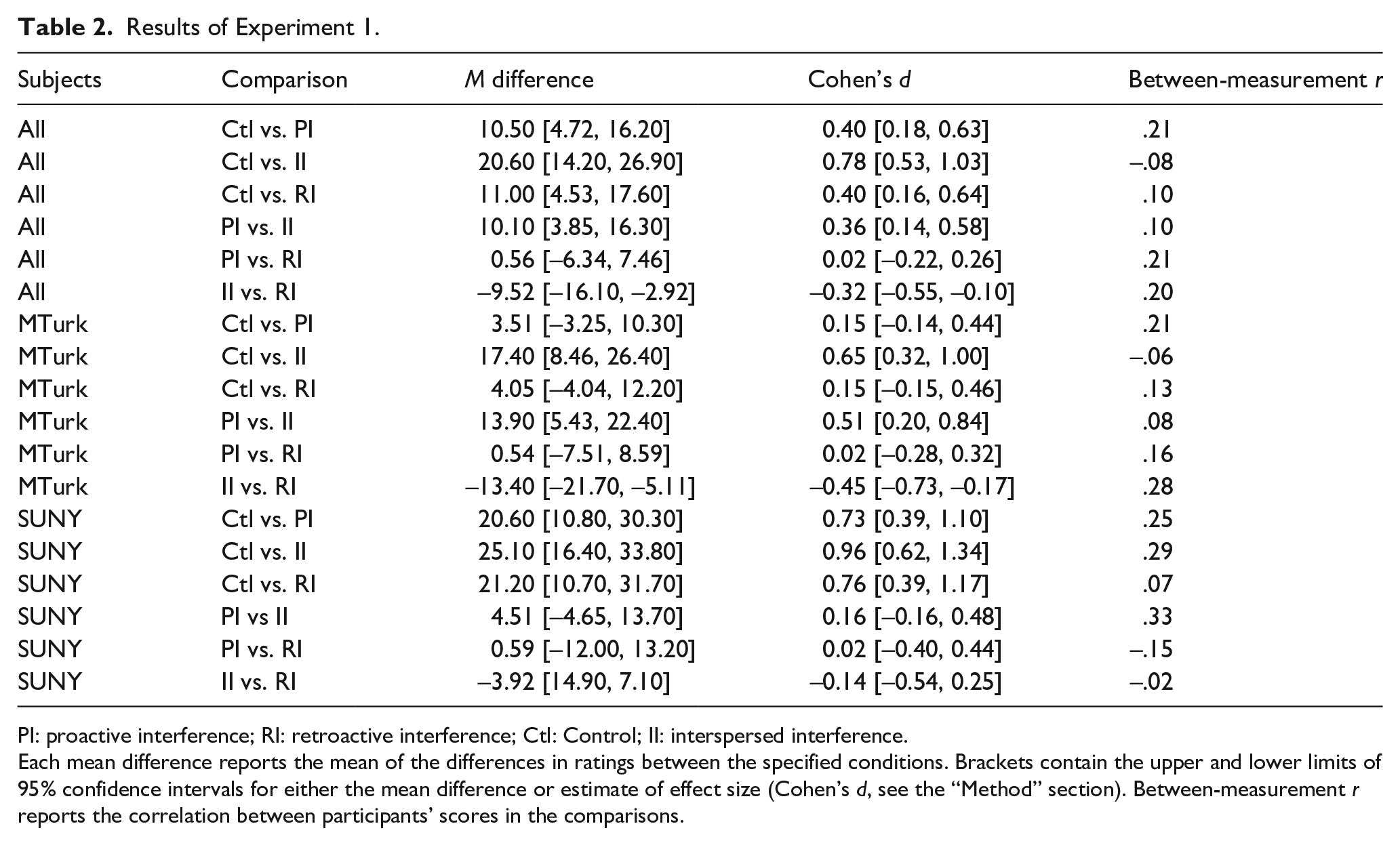
PI: proactive interference; RI: retroactive interference; Ctl: Control; II: interspersed interference.

Each mean difference reports the mean of the differences in ratings between the specified conditions. Brackets contain the upper and lower limits of 95% confidence intervals for either the mean difference or estimate of effect size (Cohen’s d, see the “Method” section). Between-measurement r reports the correlation between participants’ scores in the comparisons.

Discussion

The goal of Experiment 1 was to contrast PI, II, and RI. We expected RI to be stronger than PI because the effect of recency is ordinarily strong when testing occurs immediately after training, as was done here. This was not the case. There was no detectable difference between RI and PI.

Despite this clear-cut result, a potential problem with Experiment 1 is that participants were recruited from two different subject pools, differing considerably at least with respect to gender and age. The participants from the Binghamton pool were more often female and much younger than those recruited on MTurk, and the age distribution was also much less variable in the Binghamton sample. Murphy et al. (2021) also used a mix of subjects from those two pools with a streaming task and failed to find a difference between them. This was not the case here. An ANOVA using type of interference (Ctl vs. PI vs. II vs. RI) and subject pool (Binghamton vs. MTurk) as factors revealed an interaction, F(2.96, 364.54) = 3.22, p < .05, $η_{p}^{2}$ = .02, 90% CI = [0.002, 0.05], which indicates that the interference effects per se were different between the two populations. Notably, neither PI nor RI was detected in the sample of MTurk participants with only II having a detrimental effect on the C-O3 ratings. By contrast, the SUNY participants displayed PI, II, and RI (see Table 2). At the descriptive level, II was more efficient than either PI and RI at reducing the C-O3 ratings in these participants even though, as shown in Table 2, this difference was not statistically reliable, which is not surprising given the small sample size drawn from the SUNY-Binghamton subject pool.

The results from this analysis need to be qualified: this is a post hoc analysis that was not initially planned and which was carried out on sample sizes from each population (i.e., SUNY-Binghamton’s subject pool and MTurk) considerably below the 130 that we a priori deemed necessary for the full study. Yet, because of the ambiguities raised by apparent differences across populations, another experiment contrasting RI, II, and PI to corroborate the results from Experiment 1 seemed advisable. Instead of exactly replicating the procedure used in Experiment 1, we decided to use another version of the rapid-trial streaming procedure used previously by Jozefowiez (2021), Jozefowiez et al. (2022), and Maia et al. (2018), which was closer to the original streaming procedure designed by Allan and collaborators (Crump et al., 2007; Hannah et al., 2009; Siegel et al., 2009) and the one subsequently used by Laux et al. (2010). If we also found that II was more efficient than RI and PI in this procedure, this would indicate that the conclusions of Experiment 1 are conceptually replicable and are not dependent upon the specific populations or the procedures we used.

Experiment 2

There were six (a–f) noteworthy differences between the streaming procedure used in Experiment 1 and the one used in Experiment 2. (a) Instead of the simultaneous cue–outcome pairings of Experiment 1, the timing of cue and outcome delivery in Experiment 2 was modelled after a delay conditioning procedure with outcome onset corresponding to the cue offset; (b) the cue and outcome durations as well as the ITI were each reduced to 100 ms; (c) the same stimuli were used across all conditions instead of different stimuli being used in each condition; (d) each participant was exposed multiple times to the same condition instead of being exposed just once; (e) the warm-up phase and the question asked of participants at the end of each stream differed from those used in Experiment 1 (see “Method” section for details); and (f) in Experiment 2, the PI, II, and RI treatments took place not only in streams in which the target cue was reliably paired with the target outcome (as in Experiment 1) but also in streams in which it was not. The primary motivation for this choice was to encourage participants to use the full rating scale (the dummy conditions in Experiment 1 played the same function) and also allowed assessment of whether the relative efficacies of PI, II, and RI were a function of the target cue–outcome contingency. Thus, Experiment 2 was a 2 (number of cue–outcome pairings: High vs. Low) × 4 (Interference: Ctl vs. PI vs. II vs. RI) fully within-subjects factorial design.

Method

Participants and apparatus

All participants were screened for susceptibility to visually induced seizures and not being colour blind. Recruitment was limited to individuals between 18 and 50 years old. As in Experiment 1, we sought data from a minimum of 130 participants. Starting with 172 participants from the SUNY-Binghamton subject pool, 35 participants failed the warm-up sequence and consequently were eliminated from the experiment (see below for details). This left 137 participants (M_age: 19.24 ± 1.26, min: 18, max: 26; 55 males, 82 females). The experiment took place online using the Gorilla platform.

Procedure

Participants initially read and signed a consent form. The subsequent procedure was composed of a warm-up sequence to familiarise participants with the procedure and to screen out participants who could not meet our basic learning criterion. The warm-up sequence was itself divided into four parts: positive contingency warm-up, negative contingency warm-up, mixed contingency warm-up, and “YXZ” warm-up. The warm-up sequence was then followed by the formal experiment. The same attention screen task and distraction question used in Experiment 1 at the end of the experiment was used again to screen out participants who did not pay attention during the task.

During the experiment, participants were exposed to a series of rapid streams of trials. A stream started with a 1-s dark grey background screen with a centred, light grey, fixation cross. The background was surrounded by a patterned border (small, empty, black circles on a white background). Along with the fixation cross, this background and the border remained visible throughout the stream. This screen was followed by trials composed of (a) a 100-ms cue segment during which a trial marker stimulus (a white triangle, A), presented on every trial, was shown in the top-left corner of the screen, while another stimulus (a green circle, target stimulus X; a purple trapezoid, distractor stimulus Y; a pink parallelogram, distractor stimulus Z; or a yellow pentagram, distractor stimulus W) was potentially shown in the upper right corner; (b) a 100-ms outcome segment during which an outcome (a red square that served as the target outcome O1; a blue rhombus that served as the interfering outcome O2; an orange star that served as a distractor outcome O3; or a black chevron that served as distractor outcome O4) could be presented in the lower centre part of the screen; (c) a 100-ms ITI during which only the fixation cross plus background and border was present. Depending on the condition, target Cue X was paired with either O1 or O2, Cue W was paired with O2, Cue Y was paired with O3, and Cue Z was paired with O4. The various types of trials that could occur within a stream are depicted in Table 3.

Table 3.

List of the various trial types composing a stream in the positive and negative warm-up conditions in Experiment 2.

Trial type	Cue identity	Outcome identity
X-O1	X	O1
X-O2	X	O2
X-	X	No outcome
Y-O3	Y	O3
Y-	Y	No outcome
Z-O4	Z	O4
Z-	Z	No outcome
W-O2	W	O2
O1	No cue	O1
O3	No cue	O3
O4	No cue	O4
Empty trials	No cue	No outcome

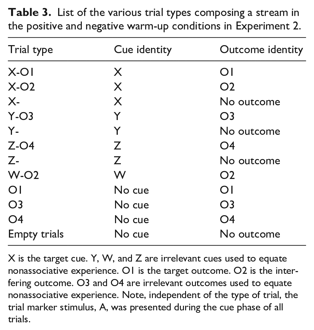
X is the target cue. Y, W, and Z are irrelevant cues used to equate nonassociative experience. O1 is the target outcome. O2 is the interfering outcome. O3 and O4 are irrelevant outcomes used to equate nonassociative experience. Note, independent of the type of trial, the trial marker stimulus, A, was presented during the cue phase of all trials.

At the end of each condition, participants were asked to rate how likely it was for X (or Y or Z) to be followed by O1 (or O3 or O4, respectively) in the stream they had just seen. The participants were shown cue X (or Y, or Z) and the trial marker stimulus A on the background screen as they appeared during the stimulus stream. Immediately above it was the statement: “Imagine you have been shown the following configuration on the screen.” Below the screenshot was the question “Using the scale at the bottom of the screen, please use the mouse to indicate how likely it was, in the sequence of stimulus you just saw, that the top configuration was followed by the lower configuration.” Below this instruction, there was an image of O1 (or O3, or O4, respectively) over the background screen as it appeared in the stimulus stream. Below this, there was an 11-point Likert-type scale ranging from 0 to 100 (incremented by steps of 10) and anchored at 0 (very unlikely) and 100 (very likely). Once participants had provided their responses on the Likert-type scale, a grey screen appeared with a dark grey button reading “Left click to continue.” This either caused the appearance of the next test question, the beginning of the next stream, or the debriefing screen at the end of the experiment. The purpose of the “Left click to continue” instruction was to ensure that the mouse was centred in the middle of the screen when a Likert-type rating appeared because the Gorilla system does not give the experimenter direct control of a participant’s mouse.

Positive warm-up

At the beginning of the positive warm-up, instructions explaining the task were presented. The instructions also asked participants to turn off their cell phones and to ensure that they would not be disturbed for the next hour. A stream was composed of 10T-O/10 empty trials, where T stands for stimulus Y, X, or Z, and O stands for O3, O1, or O4: Y was paired with O3, X with O1, and Z with O4. This implemented a ∆p = 1 contingency between T and O. The order of presentation of the streams and the order of trials within each stream was determined randomly. Once each of the three positive warm-up streams had been presented, it was followed by its test question. After all three positive streams were rated, participants were shown a single instructional screen informing them that they should have answered 100 to each of the three questions because X (or Y, or Z, respectively) was always followed by O1 (or O3, or O4). This feedback was left on the screen until the participant clicked on a button reading “Next” to start the next stream.

Negative warm-up

The negative warm-up sequence was identical to the positive warm-up streams, except that now ∆p = −1. More precisely, a stream was composed of 10 T-/10 O trials where T stands for Y, X, or Z and O stands for O3, O1, or O4: the target outcome was O3 (respectively, O1, O4) if the target cue was Y (respectively, O1, O4). The instructional screen at the end told participants that they should have answered 0 for all three questions. Then, by pressing a button reading “Next,” the participants moved to the next warm-up sequence.

Mixed warm-up

The mixed warm-up sequence started immediately after the participants had completed the negative warm-up sequence. A briefing screen informed them that they were about to see streams similar to the ones they had seen before and that they should try to identify them correctly. They were then presented with a block composed of six stimulus streams: three streams identical to the ones shown during the positive warm-up and three streams identical to the ones shown during the negative warm-up. The order of presentation of the six streams was determined randomly.

If participants provided a “correct” rating for all six of the X-O1 relationships, they moved on to the final warm-up phase. A “correct” rating after a positive (or negative) warm-up stream was defined as selecting ratings between 60 and 100 (0 and 50). If the participant made any errors by this criterion, the block of six streams was presented again. If the block was shown 10 times without the participant being 100% correct on all six ratings, the participant was rejected from the study and shown a debriefing screen thanking them for their participation.

YXZ warm-up

The YXZ warm-up sequence started right after the participants had successfully completed the mixed warm-up. During this sequence, the participants were presented with a block composed of two 3-phase streams. One stream was composed of 10 Y-O3 and 10 empty trials in Phase 1, 10 X-O1 and 10 empty trials in Phase 2, and 10 Z-O4 and 10 empty trials in Phase 3. Hence, ∆p = 1 between the target cue and the target outcome in each phase. ∆p = −1 in each phase of the other stream which was composed of 10 Y- and 10 O3 trials in Phase 1, 10 X- and 10 O1 trials in Phase 2, and 10 Z- and 10 O4 trials in Phase 3. The order of presentations of the trials within a phase was random. At the end of each stream, the participants were asked to answer three rating questions: one dealing with Y and O3, the second with X and O1, and the third with Z and O4. The order of presentation of the three rating questions was determined randomly for each stream and each participant. The order of presentation of the streams within the block was also determined randomly. If participants got the six ratings correct (same definition of “correct” as in the mixed warm-up sequence), the actual experimental portion of the study began without delay. Otherwise, the block was presented again. If the block was presented 10 times without the participant getting the six ratings right, the experiment was terminated, and the participant was eliminated from the study after being shown a debriefing screen.

Experimental streams

The experimental streams started immediately after participants had passed the YXZ warm-up sequence. A briefing screen informed them that they would now be presented with streams for which it would be more difficult to make a rating. They were also informed that the study lasted about 45 min from that point and that they would be allowed to take a break of up to 10 min roughly midway through the remainder of the study.

Participants were presented with eight blocks of streams, each containing one complete set of each of the eight conditions depicted in Table 4. These streams were identical to the ones shown during the YXZ warm-up except for the trial composition of each phase which is indicated in Table 4. The target cue and outcomes were Y and O3 in Phase 1, X and O1 in Phase 2, and X and O4 in Phase 3. Each phase was composed of a core set of 20 trials aimed at establishing a base contingency between the target cue and outcome for that phase. The target cue and outcome were shown 10 times each during this core set of trials. In Phase 1, p(O3|Y) was set to 0.5 for those core trials. This was also the case for p(O4|Z) during Phase 4. During Phase 2, p(O1|X) varied between 0.3 (low-pairing condition) and 0.7 (high-pairing condition). In the Ctl streams, in addition to these core trials, there were 20 W-O2 filler trials during each of the three phases of each stream. In the PI streams, the 20 W-O2 trials in Phase 1 were replaced with 20 X-O2 interfering trials, creating the conditions for PI of the X-O1contingency of Phase 2 by the X-O2 pairings in Phase 1. Likewise, in the II streams, the 20 W-O2 trials in Phase 2 were replaced with 20 X-O2 interfering trials, fulfilling the conditions for II. Finally, in the RI streams, the 20 W-O2 trials in Phase 3 were replaced with 20 X-O2 interfering trials, implementing the conditions for RI.

Table 4.

Composition of the streams during the experimental stage of Experiment 2.

Condition	Trial composition
Ctl—High	Ph 1: 5 Y-O3/5 Y-/5 O3/5 empty trials- (core) + 20 W-O2 (filler) Ph 2: 7 X-O1/3 X-/3 O1/7 empty trials (core) + 20 W-O2 (filler) Ph 3: 5 Z-O4/5 Z-/5 O4/5 empty trials (core) + 20 W-O2 (filler)
Ctl—Low	Ph 1: 5 Y-O3/5 Y-/5 O3/5 empty trials (core) + 20 W-O2 (filler) Ph 2: 3 X-O1/7 X-/3 O1/7 empty trials (core) + 20 W-O2 (filler) Ph 3: 5 Z-O4/5 Z-/5 O4/5 empty trials (core) + 20 W-O2 (filler)
PI—High	Ph 1: 5 Y-O3/5 Y-/5 O3/5 A- (core) + 20 X-O2 (interfering) Ph 2: 7 X-O1/3 X-/3 O1/7 empty trials (core) + 20 W-O2 (filler) Ph 3: 5 Z-O4/5 Z-/5 O4/5 empty trials (core) + 20 W-O2 (filler)
PI—Low	Ph 1: 5 Y-O3/5 Y-/5 O3/5 emptry trials (core) + 20 X-O2 (interfering) Ph 2: 3 X-O1/7 X-/7 O1/3 empty trials (core) + 20 W-O2 (filler) Ph 3: 5 Z-O4/5 Z-/5 O4/5 empty trials (core) + 20 W-O2 (filler)
II—High	Ph 1: 5 Y-O3/5 Y-/5 O3/5 empty trials (core) + 20 W-O2 (filler) Ph 2: 7 X-O1/3 X-/3 O1/7 empty trials (core) + 20 X-O2 (interfering) Ph 3: 5 Z-O4/5 Z-/5 O4/5 empty trials (core) + 20 W-O2 (filler)
II—Low	Ph 1: 5 Y-O3/5 Y-/5 O3/5 empty trials (core) + 20 W-O2 (filler) Ph 2: 3 X-O1/7 X-/7 O1/3 empty trials (core) + 20 X-O2 (interfering) Ph 3: 5 Z-O4/5 Z-/5 O4/5 empty trials (core) + 20 W-O2 (filler)
RI—High	Ph 1: 5 Y-O3/5 Y-/5 O3/5 empty trials (core) + 20 W-O2 (filler) Ph 2: 7 X-O1/3 X-/3 O1/7 empty trials (core) + 20 W-O2 (filler) Ph 3: 5 Z-O4/5 Z-/5 O4/5 empty trials (core) + 20 X-O2 (interfering)
RI—Low	Ph 1: 5 Y-O3/5 Y-/5 O3/5 empty trials (core) + 20 W-O2 (filler) Ph 2: 3 X-O1/7 X-/7 O1/3 empty trials (core) + 20 W-O2 (filler) Ph 3: 5 Z-O4/5 Z-/5 O4/5 empty trials (core) + 20 X-O2 (interfering)

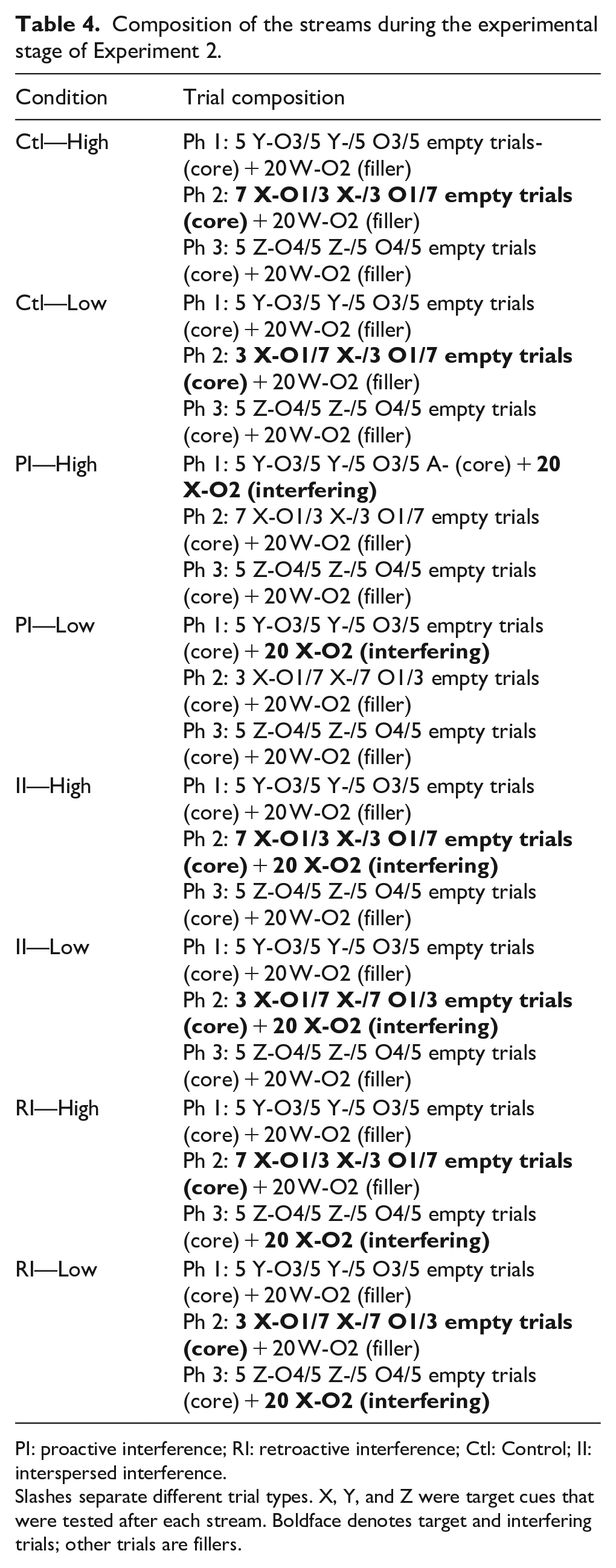
PI: proactive interference; RI: retroactive interference; Ctl: Control; II: interspersed interference.

Slashes separate different trial types. X, Y, and Z were target cues that were tested after each stream. Boldface denotes target and interfering trials; other trials are fillers.

In the terminology of contingency theory, the goal of those X-O2 trials was to degrade the X-O1 contingency by lowering p(O1|X). In the high-pairing Ctl condition, p(O1|X) was equal to 0.7 (there were 10 X trials among which 7 were reinforced with O1) with p(O1|no X), computed over all three phases of the stream, was 0.11 (30 empty trials, 3 of which are reinforced with O1). Hence, ∆p between X and O1 was 0.58. Likewise, in the low-pairing Ctl streams, ∆p between X and O1 was 0.06. Following the same calculation, in the interference streams, ∆p between X and O1 was 0.12 in the high-pairing streams and −0.13 in the low-pairing ones. Note that, because we designed the experiment to keep the outcome density constant, the number of X-O1 pairings effectively determined ∆p.

For each participant, the order of presentation of the conditions within each of the eight blocks was determined randomly and the order of the trials within each phase of each condition was determined randomly. After being exposed to four blocks, a screen appeared indicating to the participants that they could now take a break of up to 10 min. When ready, they could resume the experiment by clicking on a “Continue” button.

Attention screen task and distraction question

Once the eight blocks were completed, the participants were presented with the same attention screen and distraction question used in Experiment 1. Participants failing the attention screen (n = 1) or answering positively to the distraction question (n = 14) were eliminated from the study. All participants were then shown the same debriefing screen shown to the participants who failed the warm-up sequence.

Data analysis was conducted as in Experiment 1. All raw data are available at https://orb.binghamton.edu/jwhswcm_rawdata/1.

Results

The present section only discusses the X-O1 ratings. Results concerning the Y-O3 and Z-O4 ratings can be found in the online supplementary materials. Figure 2 shows the X-O1 ratings as a function of the number of X-O1 pairings (high vs. low) and the interference treatment (Ctl vs. PI vs. II vs. RI). A repeated-measures ANOVA using the number of X-O1 pairing (high vs. low) and the interference treatment (Ctl vs. PI vs. II vs. 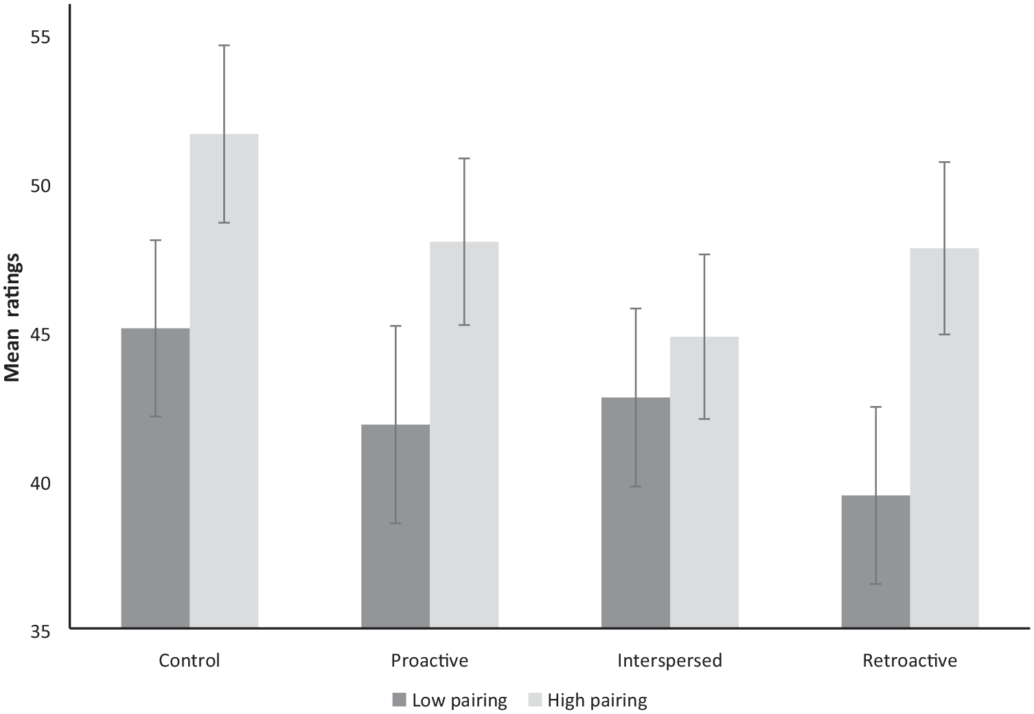RI) as factors found a main effect of the number of X-O1 pairing, F(1, 136) = 59.06, p < .001, $η_{p}^{2}$ = .30, 90% CI = [0.20, 0.39], and interference treatment, F(2.86, 389.55) = 10.86, p < .001, $η_{p}^{2}$ = .07, 90% CI = [0.03, 0.11], as well as an interaction between the two factors, F(2.97, 404.49) = 4.93, p < .01, $η_{p}^{2}$ = .03, 90% CI = [0.007, 0.06].

Figure 2.

Top: Mean X-O1 ratings as a function of the number of X-O1 pairings and the interference conditions in Experiment 2. Error bars are 95% CIs.

As shown in Table 5, in the high-pairing condition, PI, II, and RI all reduced the ratings relative to Ctl, but II was more effective at doing so than both PI and RI, whereas there was no statistically significant difference between PI and RI. In the low-pairing condition, PI, II, and RI were again all effective at decreasing the contingency rating relative to Ctl. But here, II was not the most effective treatment: as shown in Table 5, RI was more effective than II, whereas there was no significant difference between PI and II. There was also no significant difference between PI and RI.

Table 5.

Results of the X-O1 ratings in Experiment 2.

X-O1 pairings	Interference treatment	M difference	Cohen’s d	Between-measurement r
High	Ctl vs. PI	3.62 [0.84, 6.40]	0.21 [0.05, 0.37]	.54
High	Ctl vs. II	6.82 [4.12, 9.51]	0.40 [0.24, 0.56]	.56
High	Ctl vs. RI	3.84 [0.91, 6.78]	0.22 [0.05, 0.39]	.50
High	PI vs. II	3.19 [1.02, 5.37]	0.19 [0.06, 0.33]	.69
High	PI vs. RI	0.22 [–2.19, 2.63]	0.01 [–0.13, –0.16]	.64
High	II vs RI	–2.97 [–5.44, –0.51]	–0.18 [–0.33, –0.03]	.62
Low	Ctl vs. PI	3.24 [0.68, 5.80]	0.17 [0.04, 0.31]	.67
Low	Ctl vs. II	2.33 [0.18, 4.48]	0.13 [0.01, 0.25]	.74
Low	Ctl vs. RI	5.62 [3.25, 7.99]	0.32 [0.18, 0.46]	.68
Low	PI vs. II	–0.91 [–3.30, 1.48]	–0.05 [–0.18, 0.08]	.72
Low	PI vs. RI	2.38 [–0.33, 5.09]	0.13 [–0.02, 0.27]	.63
Low	II vs. RI	3.29 [1.03, 5.56]	0.19 [0.06, 0.32]	.71

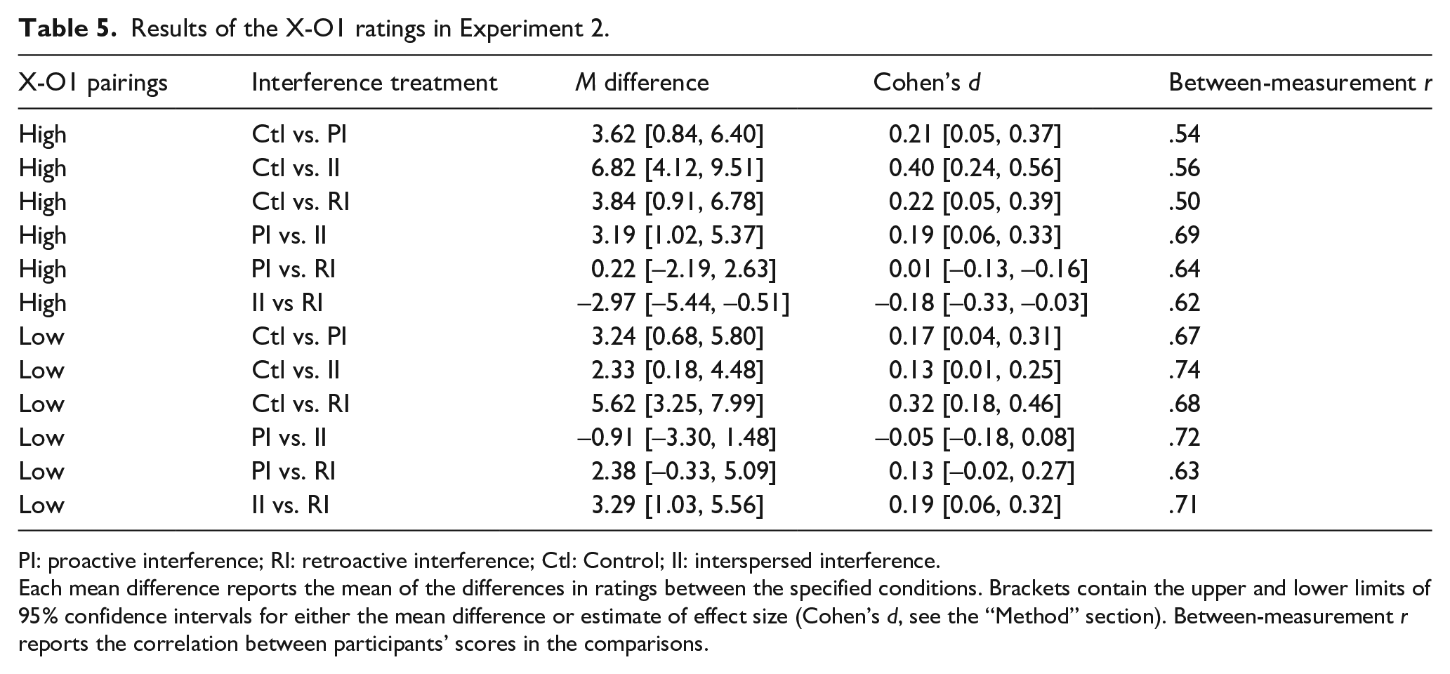
PI: proactive interference; RI: retroactive interference; Ctl: Control; II: interspersed interference.

Discussion

Experiment 2 addressed the same basic question as Experiment 1 regarding the relative efficacies of PI, II, and RI, but it used a different form of the streaming procedure. Because in Experiment 1, the number of pairings between the target cue and outcome was always high, comparisons must be restricted to the similar conditions in Experiment 2. Within this constraint, the two experiments produced similar results. First, neither experiment detected an appreciable difference between PI and RI. The other main conclusion of Experiment 1 was that II was better than either PI or RI at lowering ratings of the likelihood that the target cue would be followed by the target outcome given a strong positive baseline contingency. Experiment 2 reached the same conclusion.

In summary, Experiment 2 confirmed that, when the cue–outcome contingency is strong, II is more efficient than both PI and RI, and there is no appreciable difference between PI and RI. However, Experiment 2 went beyond Experiment 1 by including streams in which the cue was not often paired with the outcome. This revealed that the efficacy of II varied as a function of the number of X-O1 pairings. It was the most efficient treatment in the high-pairing condition, but it was outclassed by RI in the low-pairing condition.

Experiment 3

The aim of Experiment 3 was to compare the latent inhibition, partial reinforcement, and extinction effects achieved by nonreinforced presentations of a target cue alone either before (LI), among (PR), or after (Ext) cue-outcome pairings. Thus, Experiment 3 paralleled the comparisons between PI, II, and RI in Experiments 1 and 2. Due to the temporal position of the target training relative to the nontarget training (i.e., interference or nonreinforcement), one might expect parallels between PI and LI, II and PR, and Ext and RI. But Harris and Andrew (2017) have presented evidence that the consequences of cue nonreinforcement, Ext in this case, for a target cue-outcome pairing, depend uniquely on the number of trials, as opposed to encoding of the potentially cue-interfering outcome relationship for which cue duration is critical; and Stout and Miller (2007) and Wagner (1981) have theorised with some empirical support that the consequences of nonreinforcement are more dependent on cue-context pairings than cue-nontarget outcome pairings. Because the inclusion of a low-pairing condition in Experiment 2 proved informative as it revealed an interaction between interference and the number of cue-outcome pairings, Experiment 3 replicated Experiment 2, simply substituting LI, PR, and Ext for PI, II, and RI to determine whether nonreinforcement interacts with the target contingency in the same way that interference did.

Method

Participants and apparatus

The experiment was conducted online using the Gorilla experiment builder. We aimed to recruit at least as many participants as in Experiment 2. In total, 222 participants were recruited from the SUNY-Binghamton subject pool. Participants had to be between 18 and 50 years old with no prior history of epileptic seizures. 45 participants were discarded from the analysis: 26 because they failed to reach the learning criterion during the warm-up stage of the experiment, 18 because they indicated they had been distracted, and 1 because they failed the attention screen at the end of the study. This left 177 participants (41 males, 135 females, and 1 participant who preferred not to provide gender information). Ages ranged from 18 to 45 years old with an average of 18.69 and a standard deviation of 2.20. The median age was 18 years old.

Procedure and data analysis

The procedure was identical to the one used in Experiment 2. The only difference was that the interference X-O2 trials and the control trials W-O2 were replaced with nonreinforcement trials X- (i.e., X was presented but was not followed by an outcome) and control trials W- (i.e., W was shown but was not followed by an outcome). Data analysis proceeded as in Experiment 2. All raw data are available at https://orb.binghamton.edu/jwhswcm_rawdata/1.

Results

Only the X-O1 ratings will be presented and discussed here. The Y-O3 and Z-O4 ratings are treated in the online supplementary materials. Figure 3 shows the mean ratings as a function of the number of X-O1 pairings and the treatment conditions. A repeated-measures ANOVA using the number of X-O1 pairings (High vs. Low) and the nonreinforcement treatment (Ctl vs. PI vs. PR vs. 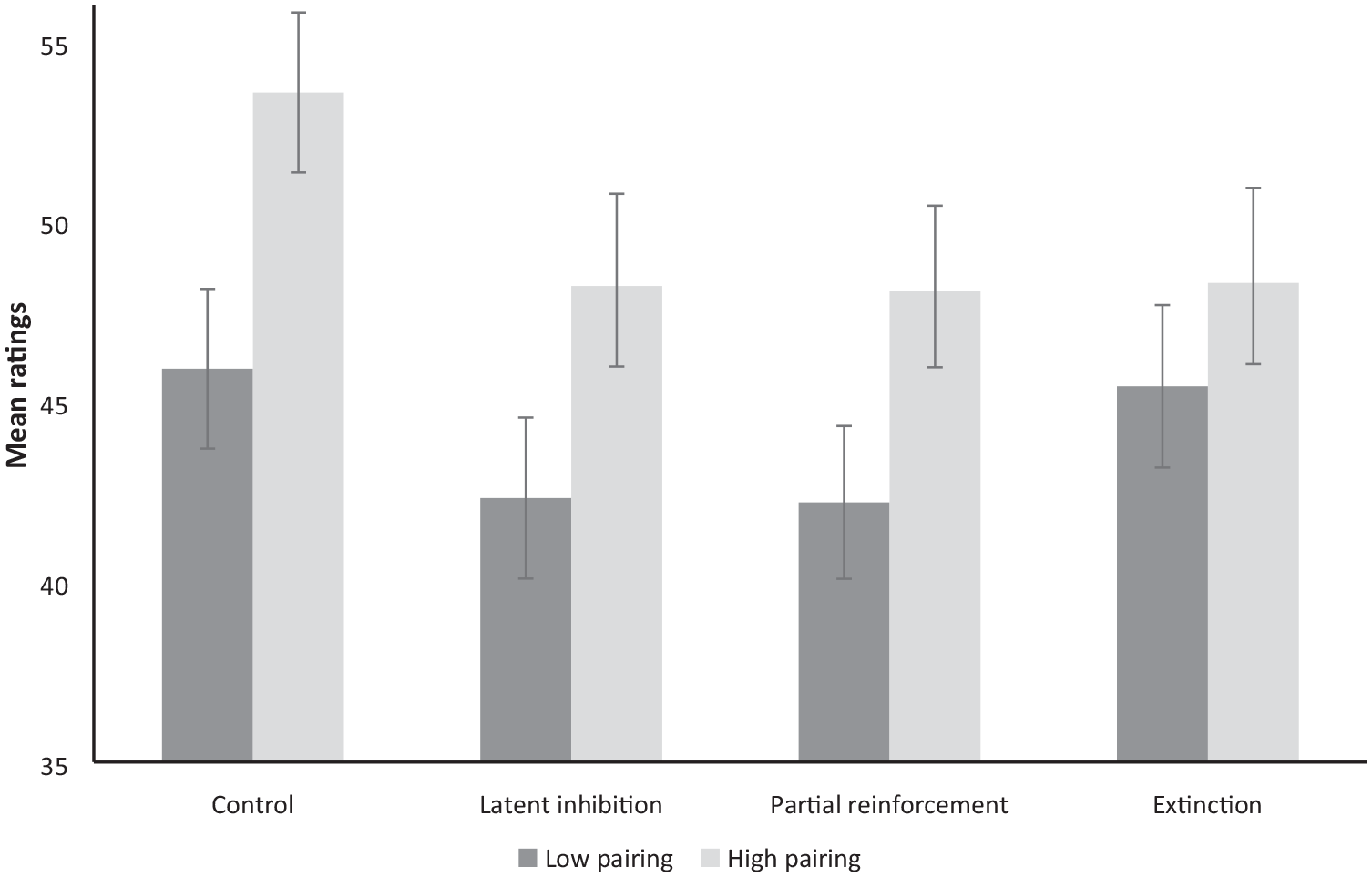Ext) as factors found a main effect of the number of X-O1 pairings, F(1, 176) = 72.67, p < .001, $η_{p}^{2}$ = .29, 90% CI = [0.20, 0.37], and the interference treatment, F(2.94, 517.49) = 12.87, p < .001, $η_{p}^{2}$ = .07, 90% CI = [0.03, 0.10], as well as an interaction between the two factors, F(2.97, 522.15) = 5.22, p < .01, $η_{p}^{2}$ = .03, 90% CI = [0.007, 0.05].

Figure 3.

Mean X-O1 ratings as a function of the X-O1 contingency and the nonreinforcement condition in Experiment 3. Error bars are 95% CIs.

As shown in Table 6, in the high-pairing conditions, ratings were lower in LI, PR, and Ext compared with Ctl. There was no detectable difference between LI, PR, and Ext. In the low-pairing conditions, only LI and PR altered the Likert-type ratings relative to Ctl or PR. Ext had no reliable impact on ratings of X-O1. Ratings were higher in Ext than in both LI and PR, whereas there was no appreciable difference between LI and PR.

Table 6.

Results of the X-O1 ratings in Experiment 3.

X-O1 pairings	Nonreinforcement treatment	Mean difference	Cohen’s d	Between-measurement r
High	Ctl vs. LI	5.37 [3.11, 7.62]	0.36 [0.21, 0.51]	.49
High	Ctl vs. PR	5.50 [3.37, 7.63]	0.38 [0.23, 0.53]	.52
High	Ctl vs. Ext	5.28 [2.88, 7.68]	0.35 [0.19, 0.51]	.42
High	LI vs. PR	0.13 [–1.63, 1.90]	0.01 [–0.11, 0.13]	.67
High	LI vs. Ext	–0.08 [–2.15, 1.98]	–0.01 [–0.14, 0.13]	.58
High	PR vs. Ext	–0.22 [–2.14, 1.71]	–0.01 [–0.14, 0.11]	.61
Low	Ctl vs. LI	3.59 [1.82, 5.35]	0.22 [0.11, 0.33]	.74
Low	Ctl vs. PR	3.71 [1.82, 5.60]	0.24 [0.12, 0.36]	.66
Low	Ctr vs. Ext	0.49 [–1.47, 2.45]	0.03 [–0.09, 0.15]	.69
Low	LI vs. PR	0.12 [–2.10, 2.34]	0.01 [–0.13, 0.14]	.59
Low	LI vs. Ext	–3.10 [–5.18, –1.02]	–0.18 [–0.30, –0.06]	.68
Low	PR vs. Ext	–3.22 [–5.40, –1.04]	–0.19 [–0.32, –0.06]	.62

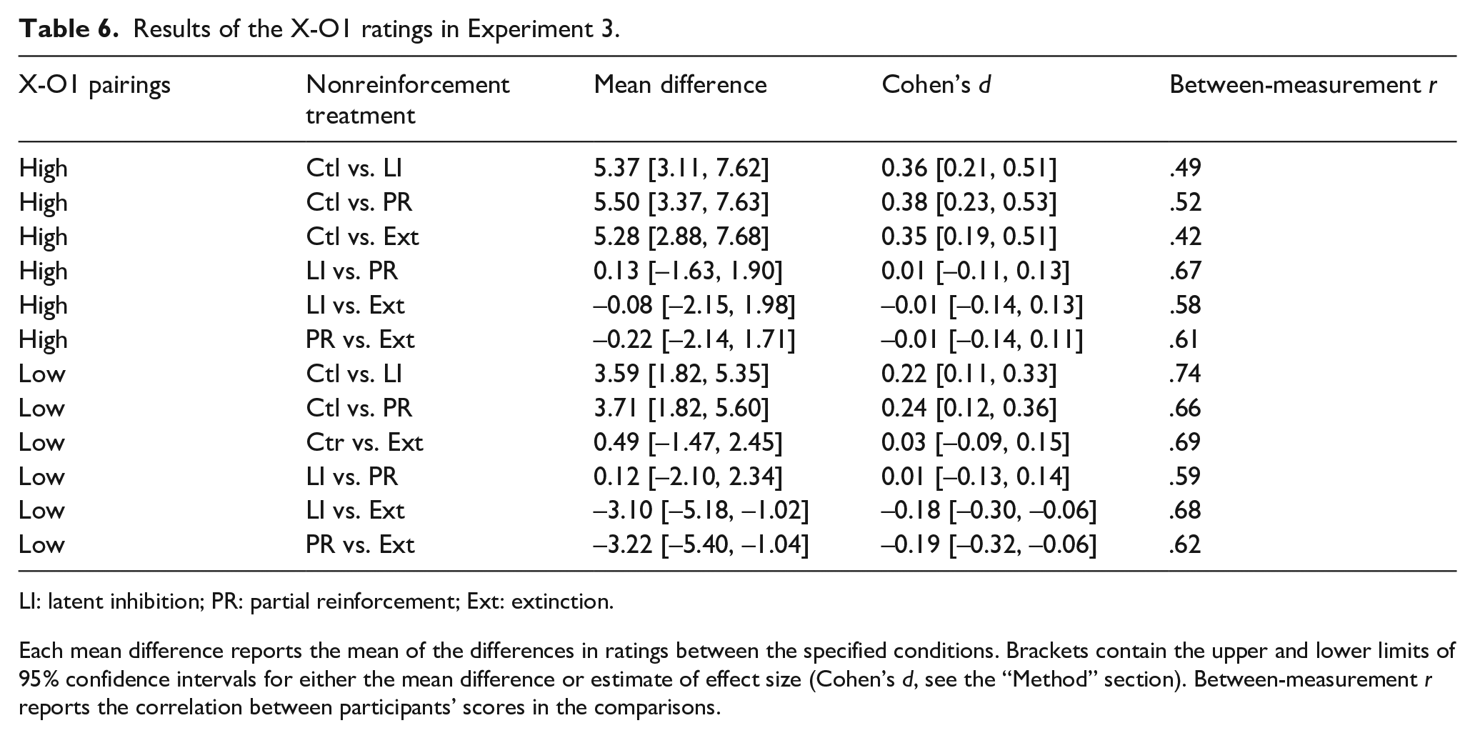
LI: latent inhibition; PR: partial reinforcement; Ext: extinction.

Discussion

Experiment 3 was designed to contrast LI, PR, and Ext using the same procedure used in Experiment 2 to contrast PI, II, and RI. Once more, the efficacy of nonreinforcement treatments varied as a function of the number of X-O1 pairings, although the pattern differed from the one observed in Experiment 2: In the high-pairing condition, there was no difference between the three nonreinforcement treatments; in the low-pairing condition, there was no difference between LI and PR while Ext was ineffective at inducing interference. This latter result might seem surprising, especially as LI and PR were able to alter the contingency rating. It will be discussed further in the “General discussion” section.

General discussion

The present experiments contrasted interference (PI, II, and RI) on one hand, and nonreinforcement (LI, PR, and Ext) on the other using the streaming procedure. Experiments 1 and 2 both found that, when the target cue was reliably paired with the target outcome, II was more efficient than either PI or RI. Experiment 2 extended this observation by showing that this result depended on the number of pairings between the target cue and the target outcome as RI proved more efficient than II when the number of pairings between the target cue and the target outcome was low. Experiment 3 also found the efficacy of nonreinforcement to be a function of the number of pairings between the target cue and outcome, but the pattern of results was quite different from the one observed in Experiment 2. Whereas II was more efficient than either PI or RI in high-pairing conditions, this was not the case for its analog in nonreinforcement, PR, in that there was no appreciable difference between LI, PR, and Ext. Moreover, whereas RI was more efficient than II in low-pairing conditions, Ext was not only less efficient than either LI and PR but seemingly had no effect at all in that it failed to degrade contingency ratings relative to Ctl.

Experiments 1 and 2 were designed to keep the outcome density constant across streams, to avoid both participants’ using this information to discriminate between streams, and potential outcome density effects (Allan et al., 2005; Allan & Jenkins, 1983). The drawback of this approach is that the X-O1 contingency (∆p) and p(O1|X) covaried. Moreover, p(O1|X) covaried with the number of X-O1 pairings. Hence, it is not possible to know whether the efficiency of interference and nonreinforcement varies as a function of ∆p (which was equal to 0.58 in the high-pairing Ctl streams and 0.08 in the low-pairing Ctl ones), p(O1|X), or the number of X-O1 pairings. Future studies will have to disentangle which of these three variables is critical to the efficiency of the various forms of interference and nonreinforcement.

That said, how can we explain the pattern of results? It is possible that the strength of the interference effect depends on the discriminability of O1 and O2 and that this discriminability is weaker in PI and RI than in II because of the greater proximity of the II interference trials to the X-O1 target trials. By this account, variables facilitating discriminability between O1 and O2 should boost the efficacy of interference. It is reasonable to assume that, when p(O1|X) is high enough, interspersing X-O1 and X-O2 trials would have such an effect in II because it provides participants with more occasion to experience O1 and O2 in close succession and hence more clearly identify the differences between them, thereby boosting its efficacy relative to PI and RI. The lower number of X-O1 trials in the low-pairing condition would attenuate any improved discriminability achieved by interspersed exposure to O1 and O2 in Phase 2. Thus, the relative efficacy of II was reduced in the case of the low-pairing contingency. PI and RI would be less affected by the contingency manipulation, because the discrimination between O1 and O2 would have already been lowered by the fact that the X-O1 and X-O2 trials never occurred in the same phase. This discrimination hypothesis would also explain why no difference was seen between LI, PR, and Ext in the high-pairing condition when X was often paired with O1, as well as between LI and PR in the low-pairing condition.

The only features of the data that the discrimination hypothesis cannot explain are the greater efficacy of RI over II in the low-pairing condition, and the lack of efficacy of Ext relative to both LI and PR in the low-pairing condition. The greater efficacy of RI over PI and II in Experiment 2 in the low-pairing condition is not surprising considering the ubiquitous nature of recency effects, in which relevant events closest to test ordinarily have the greatest impact on test performance, all other things being equal. We did indeed observe a recency effect in Experiment 2 and a hint of a recency effect in Experiment 1 (see the online supplemental materials), but Experiment 1 lacked the statistical power to properly assess it. However, the recency-effect explanation fails to account for the observations that PI and RI did not differ from each other in Experiments 1 and 2 in the high-pairing conditions and that II was stronger than either RI or PI.

If we assume that surprise is necessary for learning (Rescorla & Wagner, 1972), the lack of efficacy of Ext in the low-pairing condition might be a consequence of, in Phase 3, X- trials not being surprising anymore because participants have already experienced them extensively during Phase 2, whereas they would have remained surprising in LI and PR. Note that, in the RI condition, X-O2 trials are introduced only in Phase 3 and hence should still be surprising. That might explain why the results for the RI conditions in Experiment 2 differ from the ones observed for Ext in Experiment 3.

The above account is highly speculative, but it suggests future research concerning associative interference and nonreinforcement. Future investigation should also try to determine whether the conclusions of the present study generalise to other contingency learning paradigms, particularly ones using longer stimulus duration. It is noteworthy that the conclusions of Experiments 1 and 2 converged despite important differences in the experimental parameters, notably the stimulus duration and the contingency question. Another potential qualifier in the present study is that testing was conducted immediately after training. This leaves unanswered how PI, II, and RI would compare with LI, PR, and Ext if there was an appreciable retention interval between training and testing. In Pavlovian conditioning, recency effects (RI overcoming PI) are observed with small retention intervals, whereas primacy effects (PI overcoming RI) are more apt to be observed when an appreciable retention interval is introduced (e.g., Bouton & Peck, 1992).

Three final limitations of the present research are worth considering. First, one might be concerned that interference could have occurred across experimental conditions because of the within-subject designs that were used, especially in Experiments 2 and 3 in which the same stimuli were used in all conditions. We think that the randomisation across participants of the order of conditions within each block of conditions plus the relatively large number of participants in each experiment minimised the likelihood of this having had an appreciable effect on the present results. Indeed, Jozefowiez (2021) found no improvement in performance in participants running the streaming task daily over several months, which casts doubt on the existence of order effects in at least that version of the streaming procedure.

Second, we only explored two points on the continuum of cue–outcome contingency. In Experiments 1 and 2, the target cue was a strong predictor of the interfering outcome, whereas in Experiment 3, it was a strong predictor of the null outcome. We did not explore intermediate situations in which, for instance, the target cue would be a weak predictor of the target outcome, nor did we vary the number of pairings between the target cue and the interfering or null outcome. This would be an interesting line of research to explore in future studies.

Third, we only looked at the impact of interference and nonreinforcement on explicit cognition, that is, on explicit predictions (i.e., expectancies) made by the participants that reflect their overt knowledge of the cue–outcome contingencies. If we had used target outcomes with an emotional valence, we could have studied the impact of interference and nonreinforcement on emotions triggered by the cue as assessed, for instance, by evaluative conditioning. Jozefowiez et al. (2020) reported that the relative efficiency of extinction and counterconditioning is not the same depending on whether one assesses cognition or emotion. It is likely the same type of dissociation between cognition and emotion would have been observed here if we had used emotional outcomes. This did not prove practical. Stimuli having an emotional valence (like images from the International Affective Picture Scale) are visually more complex than the simple geometric figures we used in the present study. Hence, it would have been necessary to present them for more than 100 ms for them to be optimally processed by the participants. This would not have allowed for a fully within-subject design. Yet, in future studies, it would be interesting to examine the impact of interference and nonreinforcement on the emotional response triggered by a cue paired with an emotionally charged outcome.

Supplemental Material

sj-docx-1-qjp-10.1177_17470218231220365 – Supplemental material for Associative interference and nonreinforcement in human contingency learning

Supplemental material, sj-docx-1-qjp-10.1177_17470218231220365 for Associative interference and nonreinforcement in human contingency learning by Jérémie Jozefowiez, James E. Witnauer, Jovin Huang, Jared W. Silverstein, Samuel Woltag, Sarah Chew and Ralph R. Miller in Quarterly Journal of Experimental Psychology

Footnotes

Acknowledgements

The authors thank Audrey Huff for assistance in collecting the data and Julianna Aquilone, Kevin Artus, Nathaniel Darko, Dennis Elengickal, Allison Escaldi, Allison Hope, Audrey Huff, Dave Jiang, Sarah Landman, Jenna Polis, Jennifer Powell, and Kristina Stenstrom for their comments on an earlier version of the manuscript.

Declaration of conflicting interests

The author(s) declared no potential conflicts of interest with respect to the research, authorship, and/or publication of this article.

Funding

The author(s) disclosed receipt of the following financial support for the research, authorship, and/or publication of this article: This research was supported in part by NIH Award MH033881 and Agence Nationale de la Recherche (grant no. ANR-21-CE28-0013).

ORCID iDs

Jérémie Jozefowiez

James E. Witnauer

Ralph R. Miller

Data availability

All raw data are available at https://orb.binghamton.edu/jwhswcm_rawdata/1 or upon request from Jeremie Jozefowiez or Ralph Miller. The computer programs used to run the experiments are available at the following links: https://app.gorilla.sc/openmaterials/514512 (Experiment 1), (Experiments 2 and 3).

Supplemental material

The supplementary material is available at qjep.sagepub.com.

References

Allan

L. G.

Jenkins

H. M.

(1983). The effect of representations of binary variables on judgment of influence. Learning & Motivation, 14, 381–405.

Allan

L. G.

Siegel

Tangen

J. M.

(2005). A signal detection analysis of contingency data. Learning & Behavior, 33, 250–263.

Anwyl-Irvine

A. L.

Massonié

Flitton

Kirkham

Evershed

J. K.

(2020). Gorilla in our midst: An online behavioral experiment builder. Behavior Research Methods, 52, 388–407.

Bouton

M. E.

Peck

C. A.

(1992). Spontaneous recovery in cross-motivational transfer (counterconditioning). Animal Learning & Behavior, 20, 313–321.

Cousineau

Goulet-Pelletier

J.-C.

(2021). A study of confidence intervals for Cohen’s dp in within-subject designs with new proposals. The Quantitative Methods for Psychology, 17, 51–75.

Crump

M. J. C.

Hannah

S. D.

Allan

L. G.

Hord

L. K.

(2007). Contingency judgments on the fly. Quarterly Journal of Experimental Psychology, 60, 753–761.

Cummings

(2012). Understanding the new statistics: Effect size, confidence intervals, and meta-analysis. Routledge.

De Houwer

. (2009). The propositional approach to associative learning as an alternative for association formation models. Learning & Behavior, 37, 1–20.

Denniston

J. C.

Savastano

H. I.

Miller

R. R.

(2001). The extended comparator hypothesis: Learning by contiguity, responding by relative strength. In Klein

Mowrer

(Eds.), Handbook of contemporary learning theories (pp. 65–117). Lawrence Erlbaum.

10.

Dickinson

(1980). Contemporary animal learning theory. Cambridge University Press.

11.

Gallistel

C. R.

Gibbon

(2000). Time, rate, and conditioning. Psychological Review, 107, 289–344.

12.

Granger

R. H.

Jr. Schlimmer

J. C.

(1986). The computation of contingency in classical conditioning. In Bower

G. H.

(Ed.), The psychology of learning and motivation (Vol. 20, pp. 137–192). Academic Press.

13.

Hall

Pearce

J. M.

(1979). Latent inhibition of a CS during CS-US pairings. Journal of Experimental Psychology: Animal Behavior Processes, 5, 31–42.

14.

Hallam

S. C.

Grahame

N. J.

Harris

Miller

R. R.

(1992). Enhanced negative summation following operational extinction of a Pavlovian conditioned inhibitor. Learning & Motivation, 23, 43–62.

15.

Hannah

S. D.

Crump

M. J. C.

Allan

L. G.

Siegel

(2009). Cue-interaction effects in contingency judgments using the streamed-trial procedure. Canadian Journal of Experimental Psychology, 63, 103–112.

16.

Harris

J. A.

Andrew

B. J.

(2017). Time, trials, and extinction. Journal of Experimental Psychology: Animal Learning and Cognition, 43, 15–29.

17.

Jozefowiez

(2021). Individual differences in the perception of cue-outcome contingencies: A signal detection analysis. Behavioural Processes, 188, Article 104398.

18.

Jozefowiez

Berruti

A. S.

Moshchenko

Pena

Polack

C. W.

Miller

R. R.

(2020). Retroactive interference: Counterconditioning and extinction with and without biologically significant outcomes. Journal of Experimental Psychology: Animal Learning and Cognition, 46, 443–459.

19.

Jozefowiez

Urcelay

G. P.

Miller

R. R.

(2022). Signal detection analysis of contingency assessment: Associative interference and nonreinforcement impact cue-outcome contingency sensitivity, whereas cue density affects bias. Journal of Experimental Psychology: Animal Learning and Cognition, 48, 190–202.

20.

Laux

J. P.

Goedert

K. M.

Markman

A. B.

(2010). Causal discounting in the presence of a stronger cue is due to bias. Psychonomic Bulletin & Review, 17, 213–218.

21.

Mackintosh

N. J.

(1975). A theory of attention: Variation in the associability of stimuli with reinforcement. Psychological Review, 82, 276–298.

22.

Maia

Lefèvre

Jozefowiez

(2018). Psychophysics of associative learning: Quantitative properties of subjective contingency. Journal of Experimental Psychology: Animal Learning & Cognition, 44, 67–81.

23.

Miller

R. R.

Escobar

(2002). Associative interference between cues and between outcomes presented together and presented apart: An integration. Behavioural Processes, 57, 163–185.

24.

Miller

R. R.

Laborda

M. A.

Polack

C. W.

Miguez

(2015). Comparing context specificity of extinction and latent inhibition. Learning & Behavior, 43, 384–395.

25.

Murphy

R. A.

Witnauer

J. E.

Castiello

Tsvetkov

Alcaides

Miller

R. R.

(2021). More frequent, shorter trials enhance acquisition in a training session: There is a free lunch! Journal of Experimental Psychology: General, 151, 41–64.

26.

Nelson

J. B.

(2016). A robust function to return the cumulative density of non-central F distribution in Microsoft Office Excel. Psicológica, 37(1), 61–83.

27.

Pearce

J. M.

Hall

(1980). A model for Pavlovian conditioning; variations in the effectiveness of conditioned but not unconditioned stimuli. Psychological Review, 87, 532–552.

28.

Pineño

Miller

R. R.

(2005). Primacy and recency effects in extinction and latent inhibition: A selective review with implications for models of learning. Behavioural Processes, 69, 223–235.

29.

Polack

C. W.

Jozefowiez

Miller

R. R.

(2017). Stepping back from persistence and relapse to see the forest: Associative interference. Behavioural Processes, 141, 128–136.

30.

Rescorla

R. A.

(1967). Pavlovian conditioning and its proper control procedures. Psychological Review, 74, 71–80. https://doi.org/10.1037/h0024109

31.

Rescorla

R. A.

(1968). Probability of a shock in the presence and absence of CS in fear conditioning. Journal of Comparative and Physiological Psychology, 66, 1–5.

32.

Rescorla

R. A.

(1988). Pavlovian conditioning: It is not what you think it is. American Psychologist, 43, 151–160.

33.

Rescorla

R. A.

Wagner

A. R.

(1972). A theory of Pavlovian conditioning: Variations in the effectiveness of reinforcement and nonreinforcement. In Black

A. H.

Prokasy

W. F.

(Eds.), Classical conditioning II: Current research and theory (pp. 64–99). Appleton-Century-Crofts.

34.

Shanks

D. R.

(1995). The psychology of associative learning. Cambridge University Press

35.

Shanks

D. R.

(2007). Associationism and cognition: Human contingency learning at 25. Quarterly Journal of Experimental Psychology, 60, 291–309.

36.

Siegel

Allan

L. G.

Hannah

S. D.

Crump

M. J. C.

(2009). Applying signal detection theory to contingency assessment. Comparative Cognition & Behavior Reviews, 4, 116–134.

37.

Steiger

J. H.

(2004). Beyond the F test: Effect size confidence intervals and tests of close fit in the analysis of variance and contrast analysis. Psychological Methods, 9, 164–182.

38.

Stout

S. C.

Miller

R. R.

(2007). Sometimes competing retrieval (SOCR): A formalization of the comparator hypothesis. Psychological Review, 114, 759–783.

39.

Wagner

A. R.

(1981). SOP: A model of automatic memory processing in animal behavior. In Spear

N. E.

Miller

R. R.

(Eds.), Information processing in animals: Memory mechanisms (pp. 5–47). Lawrence Erlbaum.

Supplementary Material

Please find the following supplemental material available below.

For Open Access articles published under a Creative Commons License, all supplemental material carries the same license as the article it is associated with.

For non-Open Access articles published, all supplemental material carries a non-exclusive license, and permission requests for re-use of supplemental material or any part of supplemental material shall be sent directly to the copyright owner as specified in the copyright notice associated with the article.

0.00 MB

0.05 MB